Heuristics Assisted Set Based Data Dependence Profiling.

ABSTRACT

PARLE, APOORV. Heuristics Assisted Set Based Data Dependence Profiling. (Under the direction of Dr. James Tuck.)

Speculative optimizations unlock performance by relaxing conservative constraints

which restrict various optimizations. Data dependence profiling enables such speculative

optimizations by providing the runtime dependence profile, but most of the profilers suffer

from very large performance overhead. Recent work on set-based profiling with software

signatures has demonstrated potential to achieve low performance overhead for profiling.

But this technique suffers from very poor accuracy in some of the evaluated benchmarks,

and has scope for improvement in accuracy as well as performance overhead.

First some heuristics are introduced to predict load-store relations which are expected never to happen. These heuristics are pruned from the list of load-store relations that are

profiled, thus reducing the performance overhead by 10% on average (geometric mean).

Moreover, owing to the simplicity of the heuristics, the relations are predicted much more

accurately, than as profiled by a software signature based profiler. This results in improved

accuracy as the Normalized Average Euclidean Distance (NAED), with respect to perfect

profiler, reduces from 0.09 to 0.06 on average across all benchmarks.

Next we introduce an alternative range based set representation, as a high-speed albeit

approximate mechanism. This set representation is combined with software signatures to

create a hybrid set representation, for a highly accurate profile. In addition, short-circuit optimization is built into the hybrid set reducing the performance overhead in some

bench-marks. Combining this with the heuristics yields the most accurate profile so far, with the

average NAED of 0.04 in comparison to the perfect profiler. The combined effect of the

two also reduces the performance overhead of the profiler by 17%, on average (geometric

© Copyright 2016 by Apoorv Parle

Heuristics Assisted Set Based Data Dependence Profiling

by Apoorv Parle

A thesis submitted to the Graduate Faculty of North Carolina State University

in partial fulfillment of the requirements for the Degree of

Master of Science

Computer Engineering

Raleigh, North Carolina

2016

APPROVED BY:

Dr. Gregory Byrd Dr. Huiyang Zhou

Dr. James Tuck

DEDICATION

BIOGRAPHY

The author pursued his Bachelor’s degree in College of Engineering, Pune, majoring in

Electronics and Telecommunication. After completing his undergraduate degree, he joined

Texas Instruments Inc. as a design engineer, and worked there for 3 years. Subsequently, he

started his Master’s degree in Computer Engineering at North Carolina State University in

ACKNOWLEDGEMENTS

I would like to thank my advisor for all the indispensible guidance and help, without which

this work would not have been possible. Also, I would like to thank all my professors who

have taught me various courses, and thus enabled me to do this research. Lastly, I’ll also

acknowledge my friends and family who supported me directly or indirectly, along the

journey of M.S.

This material is based upon work supported by the National Science Foundation under

TABLE OF CONTENTS

LIST OF TABLES . . . vii

LIST OF FIGURES. . . viii

Chapter 1 Introduction. . . 1

1.1 Data Dependence Problem . . . 1

1.1.1 Data Dependence . . . 1

1.1.2 How it limits optimizations . . . 2

1.2 Data Dependence Profiling . . . 3

1.3 Background . . . 4

1.3.1 Shadow Memory based Profiling . . . 4

1.3.2 Pattern-driven Profiling . . . 5

1.3.3 Offloading Profiling for Efficiency . . . 5

1.3.4 Set-based Profiling . . . 5

1.4 Profiling Cost . . . 6

1.5 DDP Design Trade-offs . . . 6

1.5.1 Object Granularity . . . 6

1.5.2 Code Region Granularity . . . 7

1.5.3 Flow Sensitivity . . . 7

1.5.4 Call Graph Sensitivity . . . 7

1.5.5 Memory vs. Compute . . . 8

1.5.6 Coverage . . . 8

Chapter 2 Set Profiling . . . 10

2.1 How it works . . . 11

2.1.1 Query Identification . . . 11

2.1.2 Set Assignment . . . 11

2.1.3 Instrumentation . . . 11

2.2 Bloom Filter Sets . . . 13

2.2.1 Bloom Filter Design Trade-offs . . . 15

2.3 Fast Set Profiling . . . 15

2.3.1 Static Alias Analysis . . . 15

2.3.2 Diverging Control Paths . . . 16

Chapter 3 Infrastructure and Evaluation . . . 18

3.1 Set Implementation . . . 20

3.1.1 Signature Configurations . . . 20

3.2 Accuracy . . . 22

3.2.2 Normalized Average Euclidean Distance . . . 22

3.3 Experimental Setup . . . 23

3.4 Evaluation . . . 23

Chapter 4 How to Improve . . . 28

4.1 What to profile . . . 28

4.2 Set Representation . . . 29

Chapter 5 Heuristic Pruning . . . 30

5.1 Heuristics . . . 31

5.1.1 Constant Data Space . . . 31

5.1.2 Structure Type Mismatch . . . 31

5.1.3 Structure Index Mismatch . . . 33

5.1.4 Local Variables vs. Unknown Aggregates . . . 33

5.1.5 Local Structures vs. Function Arguments . . . 34

5.1.6 Local Variables with No Pointers . . . 35

5.2 Evaluation . . . 37

Chapter 6 Range Sets and Hybrid Sets . . . 44

6.1 Range Set . . . 44

6.2 Hybrid Set . . . 46

6.3 Evaluation . . . 47

Chapter 7 Conclusion . . . 51

7.1 Future Work . . . 53

LIST OF TABLES

Table 3.1 Design choices taken in our implementation . . . 21 Table 3.2 Signature Configurations . . . 21

LIST OF FIGURES

Figure 2.1 A simple bloom filter with 8 bits, and two hash functions. . . 14

Figure 2.2 Control graph with diverging paths . . . 16

Figure 3.1 Work Flow for set profiling and feedback directed optimizations . . . 19

Figure 3.2 Accuracy of the profiler with different signature configurations.[lower is better] . . . 24

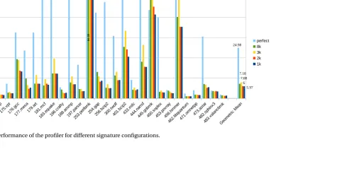
Figure 3.3 Performance of the profiler for different signature configurations. . . 26

Figure 5.1 Distribution of different heuristics on each benchmark, as a percent-age of total queries. . . 38

Figure 5.2 Accuracy observed with Signatures on only those queries which can be statically predicted with the heuristics.[lower is better] . . . 39

Figure 5.3 Accuracy for various benchmarks with and without the heuristics. [lower is better] . . . 41

Figure 5.4 Performance overhead on various benchmarks with and without the heuristics. . . 42

Figure 6.1 Operation of the range set: “a)” to “c)” show insertion and “d)” shows membership check. . . 45

Figure 6.2 Accuracy of Range and Hybrid Sets.[lower is better] . . . 48

Figure 6.3 Performance of Range and Hybrid Sets . . . 49

CHAPTER

1

INTRODUCTION

Moore’s law is slowing down, while the programs are getting bigger and bigger, increasing

the importance of optimizing softwares for good performance. In software or compiler

optimizations, only a limited amount of information is available at compile-time, limiting

the scope of optimizations. Prior works have shown that leveraging runtime information

speculatively can provide significant performance boost. One of the key factors for both

compile-time optimizations and parallelization is the ability to distinguish independent

memory references, or memory disambiguation.

Data Dependence Problem

Data Dependence

When a particular instruction depends on the result of a sequence of instructions, it is

1.1. DATA DEPENDENCE PROBLEM CHAPTER 1. INTRODUCTION

be tricky when the dependence flows through the memory.

Code Snippet 1.1Simple Data Dependence

1 R1 = R2 + 3

2 STORE R1 ,@[R3] 3 R4 = LOAD @[R3]

In Code Snippet 1.1 there is a data dependence from R2 to R1. Also, there is a dependence

from R1 to R4 which flows through memory. Because the address being used here is exactly

the same, the dependence relation is straightforward.

Code Snippet 1.2Ambiguous Memory Dependence

1 R1 = R2 + 3

2 R3 = R1 + 2

3 R4 = R1 + 3

4 STORE R6 ,@[R3 + 1] 5 R7 = LOAD @[R4]

In Code Snippet 1.2, there is a data dependence from R6 to R7. But here, the dependence relation cannot be obtained without the prior knowledge of R3 and R4. As programs get

more complicated, the relations between the memory addresses become too complex or

completely impossible to track.

How it limits optimizations

If we can clearly prove that two memory operations are independent, it gives us the freedom

to move them independently in the code. Not only the specific two instructions but all their

dependent instructions may be considered for restructuring.

Code Snippet 1.3Potential LICM opportunity

1 i n t myfunc (i n t _∗a , i n t _∗b , i n t _∗c ) {

2 i n t tmp ;

3 f o r(i n t i=0; i<1000000; i++) {

1.2. DATA DEPENDENCE PROFILING CHAPTER 1. INTRODUCTION

5 _∗b += (_∗a ) + c[ i]_∗tmp ;

6 }

7 }

Code Snippet 1.3 presents a typical Loop Invariant Code Motion (LICM) opportunity. Here,

if we can prove thataandbboth point to different memory locations, the calculation of

tmpcan be done outside the loop. But since this information is unavailable, the compiler will conservatively generate a code wheretmpwill be calculated for each iteration, even if

the exact same value, decreasing the performance significantly.

Data Dependence Profiling

In order to disambiguate such cases, runtime information has to be captured through

pro-filing. Profiling is the technique of inserting extra code to capture the required information.

Code Snippet 1.4 shows the profiled version of the Code Snippet 1.2.

Code Snippet 1.4Simple Profiling

1 R1 = R2 + 3

2 R3 = R1 + 2

3 R4 = R1 + 3

4 PROFILE_STORE ( R3+1 , ID1 ) 5 STORE R6 ,@[R3 + 1]

6 PROFILE_LOAD ( R4 , ID2 ) 7 R7 = LOAD @[R4]

Each memory operation is tagged with an unique identifier – represented here by ID1 and

ID2. The identifier is passed to the PROFILE_LOAD or PROFILE_STORE function along with

the address obtained at runtime. These functions are typically library calls which update

the data structure used to track various dependence relations. Since this snippet can be a

part of a loop, the touched memory locations can be quite large, and hence they have to be

maintained in a large data structure. Because loads and stores are common events and at each of these events such large data structures are being manipulated, data dependence

1.3. BACKGROUND CHAPTER 1. INTRODUCTION

Background

Quite a lot of work has gone into profiling data dependences[Bru00; Che04; Fax08; Kim10; VT12; Wu08; YL12b; Zha09]. At a high level, the approaches taken to track these memory locations can be classified as follows:

Shadow Memory based Profiling

This is the traditional approach, best described in[Che04], and used in many prior works [SM98; Liu06; Udu11]. The aim is to locate the closest prior instruction(s) which the current instruction depends on. As illustrated by Chen et al., a single data structure which is a

representative of the whole memory space is used to keep track of the edges. Each location

in the shadow memory, keeps track of the memory operations that have accessed it. Profiling

operations corresponding to each load and store update this shadow memory with their unique IDs (assigned statically for all memory operations). Every new operation thus forms

a link in the chain, and replaces the old value as the head in the shadow memory.

The shadow memory can be implemented as a virtually unlimited hash-table (limited by

the size of the main memory), keeping track of all previous operations. Alternatively, to limit

the size of shadow memory, a fixed width hash-table can also be used, which maintains

fixed number of prior accesses per memory location. New entries replace old entries as

they occur, while edges are recorded separately for later usage.

Irrespective of the number of operations tracked per address, the length of the

hash-table has to be limited to a fixed length. This causes multiple addresses to alias in the shadow memory, creating false dependence edges between completely independent instructions.

The biggest downside of such an approach is that if a handful number of memory

operations inside a loop access a very large number of addresses, they end up polluting the

whole hash-table. Now, completely unrelated memory operations also cannot be separated

out, resulting in very poor accuracy of profiling. And even with a fixed length hash-table,

each access and update involves a high operational overhead per memory operation.

1.3. BACKGROUND CHAPTER 1. INTRODUCTION

Pattern-driven Profiling

Pattern driven profilers[Bru00; Kim10]focus on very specific dependences in loops, looking for access patterns like strides or inter-iteration dependences. They trade-off the coverage

of the whole program with high-resolution tracking of fewer memory operations inside

hot loops. Rather than just detecting simple presence of edges, such techniques try to

determine which iteration such dependences will occur in, and which iterations can be parallelized. Owing to the high-resolution tracking of load-store pairs, such mechanisms

are very expensive.[Kim10]suggests parallelizing the profiling tasks to bring down the overhead to only 10-20x slowdown with the help of 32 cores. Due to its high-resolution,

such a technique is compelling, but the cost of required hardware resources limits its

proliferation to broader applications.

Offloading Profiling for Efficiency

A variety of prior works[Kim10; YL12b]try to offload the profiling tasks for efficient program analysis, relying on parallelism to make the profiling cheap. Various techniques like slicing [YL12a; YL12b]and novel parallel algorithms[Kim10]have been proposed. Because the memory access pattern within a program’s dynamic execution sequence is rarely balanced,

it becomes a challenge to balance the workload across different threads, for best efficiency. Moreover, dedicating large amount of resources just for profiling is not practical for many

developers.

Set-based Profiling

In this approach, each memory operation or a group of memory operations use a separate

data structure, called a set, to keep track of the addresses visited. This ensures that unrelated

memory operations do not cause any interference with each other. The expectation here

is that individual memory operations will not visit a lot of memory locations, and hence

1.4. PROFILING COST CHAPTER 1. INTRODUCTION

Profiling Cost

At a high level, with any approach, the cost of profiling can be divided into following

components:

1. Initialization: The cost of initializing the data structure(s) used to detect edges, as

well as the data structure(s) which track the profiled edges.

2. Profile Operation: The actual cost of profile operation, which includes searching

and updating the associated data structure. This is usually the main source of the

performance overhead. It also includes the cost of updating the dependence edge

counters with the recognized edges.

3. Destruction: The cost of post-processing the data structure, recording all the final

results to file/database, and de-constructing the data structure.

4. Indirect Effects: Profiling can affect the existing program execution indirectly in many

ways like cache pollution, branch predictor pollution, core IPC performance due to

data structure updates etc.

All these costs have to be accounted for when building a profiling mechanism.

DDP Design Trade-offs

In addition to the above-mentioned costs, following trade-offs also have to be considered.

The corresponding design choices taken in our implementation are presented Table 3.1 in

chapter 3.

Object Granularity

Profiling, similar to Alias Analysis, can be designed to track memory objects at various

granularities – just as bytes, simple data types or even complex structures. Usually, memory

addresses are tracked, while data type granularity is augmented statically. But with this

1.5. DDP DESIGN TRADE-OFFS CHAPTER 1. INTRODUCTION

profiling a load to store relation with addresses can suggest whether they access the same

location or not. But if the addressed location is a structure, just tracking the addresses is

not sufficient to determine if a portion of object has been updated, as that portion can

have a different address (offset by few bytes). In order to track relations at the granularity of

aggregates, the size of the access and its nesting inside an aggregate data structure has to

be tracked along with the address (which can be complicated).

Code Region Granularity

It is essential to track the edges only in relevant regions of the code. Memory operations corresponding to a loop iterator are relevant only inside the loop. In a nested loop, the inner

loop iterator will start afresh with each iteration of the outer loop, and edges corresponding

to the inner iterator seen across iterations of the outer loop can be misleading. Similarly,

edges corresponding to local variables inside a function might not be relevant when seen

across different calls to same function.

Flow Sensitivity

The flow pattern of an edge can be an essential design choice for a profiler, as it affects

what optimizations can use this data. Various options include, just the presence of an

edge, probability of the edge, or even high resolution data like stride of the inter-iteration

dependence. Different optimization rely on different profiles: LICM will utilize just the presence of the edge, while other loop optimizations like loop vectorization can utilize the

probability of the edges as well the stride of the inter-iteration dependence.

Call Graph Sensitivity

Profiling the data dependences separately for each call context can be useful to track

variation caused due to differences in inputs at various call sites. This information is highly

relevant for optimizations which specialize functions for various call sites. But this involves

tracking multiple call contexts as well as separate data structures to store edge data per

1.5. DDP DESIGN TRADE-OFFS CHAPTER 1. INTRODUCTION

Memory vs. Compute

The amount of memory used by the profiler vs. the amount of computations that have to be

performed per memory operation is a choice directly affecting the performance overhead.

The computations per profiling operation directly add to the performance overhead. The

memory usage on the other hand does not directly add to the overhead, but can be limiting

factor for a memory intensive applications. Additionally it also contributes to the overhead in the form of allocation, initialization and access (which translates to cache pollution).

Coverage

Which memory operations to profile is a design choice dependent on the optimization

passes that consume the profile data. Profiling memory operations only relevant to specific

optimization reduces the amount of profiling required, but the obtained profile is useless

anywhere else but that optimization. On the other hand, profiling all the memory operations

ensures that the obtained profile is useful for all the optimizations. How often to profile

is another aspect of coverage that needs to be considered. Sampling[Che04]is a method where not all dynamic instances of a memory operation are profiled; a profile is taken

everyn executions of the code region. Higher the frequency of sampling, better will be

the accuracy of the results, but higher will be the overhead – thus a classic accuracy vs. performance trade-off.

Many prior works[Du04; BF02; CW03; Udu11; Xek09; Wu08; Fah05; PO05; Kel09; Opl99; Kre00; Per00; Luk95; Con97; Joh04; Qui05; Liu06; BS06; Lin06; Tuc08; Bru00; Din07; Li05;

Lin03; SM98; Hwu93]have highlighted the importance of data dependence profiling, to achieve efficient optimizations or parallelization on novel high performance architectures.

Unlike edge profiling, which has been widely used due to simplicity, data dependence

pro-filing has been severely limited due to its high cost. This in turn has limited the research and

progress in the area of application specific optimization as well as speculative architecture design. Improvements in this area will translate to near term advancements like speculative

optimizations in compilers, as well enable research on novel speculative hardware designs

1.5. DDP DESIGN TRADE-OFFS CHAPTER 1. INTRODUCTION

In this dissertation, the existing technique of set based profiling has been extended, to

improve the accuracy while either maintaining or improving the performance overhead.

Next chapter will explain set based profiling and its evaluation. Subsequent chapters will

talk about different optimizations on top of set profiling, to improve its performance as

CHAPTER

2

SET PROFILING

As described in the previous chapter, conventional approach to dependence profiling

utilizes a single global structure which is a representative of the memory space. Vanka &

Tuck propose set profiling in[VT12], which creates small sets per instruction (or group of instructions), to track their memory references. These sets can be visualized as simple

mathematical sets where each element is a memory address. Any new address, visited by

the instructions corresponding to the set, is “inserted” into the set, and any instruction

which needs to be disambiguated, is “checked for membership” in that set. Sets have two

main advantages:

1. No interference from one set to another, irrespective of how many addresses are

inserted in one set.

2. Since the number of addresses inserted will be relatively small, accessing the data

2.1. HOW IT WORKS CHAPTER 2. SET PROFILING

How it works

The Set Profiler has three main stages:

Query Identification

The basic unit of granularity in a set profiler is a query, similar to querying a typical Alias

Analysis pass. When two memory operations need to be disambiguated against each other,

they form a query, which is then assigned a unique reference identifier (refid). The LHS and

RHS of the query can be arbitrary memory operations, but our implementation forms a

query with a load instruction as LHS and store instruction as RHS. All such queries which

need to be resolved, are collected for the program under consideration.

Set Assignment

Once all queries have been gathered, each of them is assigned a set, allowing the freedom

to group multiple queries into a single set. A simple grouping policy assigns all queries with

same RHS (or alternatively LHS) to a single set. Multiple RHS (or LHS) can also be grouped together arbitrarily to reduce the number of sets, but at the cost of interference from each

other. Various grouping policies can be explored in order to combine queries, such that

they will cause least interference with each other.

Instrumentation

Once all sets are obtained, the code is instrumented to perform the following:

1. Initialize all the sets as empty, at the beginning of the regions of the code where they

are used. In our implementation we do this at function boundaries by initializing the

sets on a stack.

2. Perform set insertions at all the instructions corresponding to each set.

3. Perform set membership checks to disambiguate the instructions corresponding to

2.1. HOW IT WORKS CHAPTER 2. SET PROFILING

4. Update dependence edge counters whenever an edge is detected.

Here is an example that illustrates this. Code Snippet 2.1 shows a function that needs to

be profiled. Irrelevant details of the function have been skipped for the sake of illustration.

Code Snippet 2.1Unprofiled code (written in LLVM Intermediate Representation[Llv])

1 d e f i n e i 3 2 @myfunc ( ) #0 { 2 . . .

3 BasicBlock3 : 4 . . .

5 s t o r e i 3 2 %6, i 3 2∗ %someAddress , a l i g n 4 6 . . .

7 %20 = load i 3 2_∗ %unknown , a l i g n 4 8 . . .

9 . . . 10 }

Code Snippet 2.2Same code with set profiling (written in LLVM Intermediate Representation

[Llv])

1 d e f i n e i 3 2 @myfunc ( ) #0 { 2 %s e t = c a l l i 8∗ @ a l l o c a t e S e t ( ) 3 %dependence = a l l o c a i32 , a l i g n 4

4 s t o r e i 3 2 0 , i 3 2_∗ %dependenceCounter , a l i g n 4 5

6 . . .

7 BasicBlock3 : 8 . . .

9 c a l l void @ i n s e r t (% s e t , %someAddress ) 10 s t o r e i 3 2 %6, i 3 2_∗ %someAddress , a l i g n 4 11 . . .

12 %dep = c a l l i 3 2 @membershipCheck(% s e t , %anotherAddress ) 13 %old = load i 3 2_∗ %dependence , a l i g n 4

2.2. BLOOM FILTER SETS CHAPTER 2. SET PROFILING

15 s t o r e i 3 2 %new , i 3 2_∗ %dependence , a l i g n 4 16 %20 = load i 3 2_∗ %anotherAddress , a l i g n 4 17 . . .

18 . . .

19 ; 123456 i s the r e f i d o f the query

20 c a l l void @storeQueryResults ( i 3 2 123456 , %dependence ) 21 c a l l void @deleteSet (% s e t )

22 }

Code Snippet 2.2 shows the profiled version of the function shown in Code Snippet 2.1.

For the load and store instruction that need to be disambiguated, a set has been allocated at

the very beginning of the function. Next a dependence tracking variable has been allocated

and initialized to zero. Whenever the store instruction executes, the address is inserted

into the set. Whenever the load instruction executes, the particular address is checked for

membership in the set, and the dependence tracking variable is updated accordingly. It does

not matter whether the profiling is performed before or after the load or store instruction. For the sake of consistency, we’ve chosen to always do it before the instruction. Finally

when the function completes, the dependence results are stored, and the set is deallocated.

The next section will cover how to efficiently represent sets and perform operations on

them.

Bloom Filter Sets

In order to maintain a low cost of profiling, the set operations – allocation, insertion,

mem-bership checks and deallocation have to be fast. Moreover, since there can be a lot of sets

in a program, each set should have a small memory footprint. Vanka & Tuck have proposed

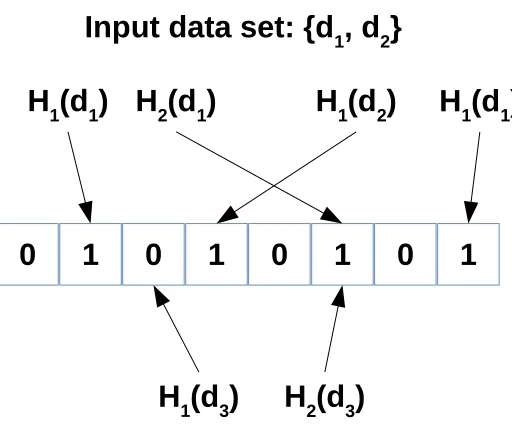
bloom filter based “software signatures”[VT12]to achieve this. A bloom filter[Blo70]is a probabilistic representation of large amount of data into a much smaller space. It is a simple

array of bits which is indexed using hash functions. Figure 2.1 shows an example bloom

filter with 8 bits. The input data set has two elementsd1andd2which need to be inserted.

2.2. BLOOM FILTER SETS CHAPTER 2. SET PROFILING

0

1

0

1

0

1

0

1

Input data set: {d

, d

}

H

(d

) H

(d

)

H

(d

)

H

(d

)

Membership Check (d

) = False

H

(d

)

H

(d

)

Figure 2.1A simple bloom filter with 8 bits, and two hash functions.

index into the bit array, and the corresponding bits are set. For a membership check, again

the hash functions are used to calculate the index, but now the bits are checked whether

they are set. If even one of the bits is not set, the membership check is deemed false. In

the current example, ford3, the bit corresponding toH1is not set, and hence it fails the

membership check.

An alternate design is to use banked bloom filters. Here the bit array is split into banks,

and a different hash function is used for each bank. This simplifies the design as each hash

function accesses a much smaller range of bits, and each bank is accessed by only one

hash function. Further, because only one hash function can access each bank, there is no interference between different hash functions. Such a design would be referred to as

2.3. FAST SET PROFILING CHAPTER 2. SET PROFILING

Bloom Filter Design Trade-offs

In order to use bloom filters for set profiling, following factors have to be taken into

consid-eration:

1. Larger the size of the bloom filter, better is the accuracy. But the size of the bloom

filter corresponds to the amount of extra memory needed for the profiling, which

translates to following cost

• Larger the memory has to be cleared during initialization.

• Since the set operations are interleaved with actual application execution, the

cache locality of the original application is affected.

2. The hash functions cannot be too complex since they have to sequentially execute on

the CPU and they have to be computed for every memory operation. Furthermore, the

input data to a typical set does not follow a purely random distribution, but instead,

a very localized distribution dependent on the application being profiled. This has to

be taken into account while tuning the hash functions.

3. The number of banks in the bloom filter (or additional hash functions) provide

addi-tional accuracy. But they also directly correspond to the amount of work that needs

to be performed per set operation.

Fast Set Profiling

The set based profiling approach allows us the freedom to selectively profile portions of the

program. This opens up some opportunities to reduce the profiling work.

Static Alias Analysis

Compilers perform Static Alias Analysis, which broadly classifies queries into MustAlias,

MayAlias and NoAlias. The MustAlias and NoAlias relations are definite relations that can

2.3. FAST SET PROFILING CHAPTER 2. SET PROFILING

the queries which can be proven statically, and only profile queries which have a MayAlias

relation.

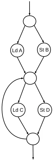
Diverging Control Paths

A program presents many different control paths, and a lot of paths are mutually exclusive.

Figure 2.2 shows an example control graph of a program. Here the instructions “Ld A”

Ld A

Ld C St D St B

Figure 2.2Control graph with diverging paths

and “St B” are present on different control paths. They can both never occur during single

instance of execution, and hence need not be profiled. The instructions “Ld C” and “St D”

are also present on different control paths, but they are present inside a loop. Even though they can never occur in the same iteration of the loop, they may have data dependence

2.3. FAST SET PROFILING CHAPTER 2. SET PROFILING

The next chapter will discuss the implementation of the set profiling infrastructure and

CHAPTER

3

INFRASTRUCTURE AND EVALUATION

The memory dependence profiling can be performed at three stages:

1. ISA/Binary Instructions

2. Intermediate Representation

3. High Level Language

Profiling at the level of a high level language has a downside that we’ll profile potentially

unnecessary information. As the program passes through optimizations, many memory operations will be promoted to register operations based on statically available information.

On the other extreme, profiling the binary instructions is again a waste as almost all the

high-level information is lost. And any subsequent information needed by the

optimiza-tions will be unavailable. Also, the registers which are spilled to memory operaoptimiza-tions are

CHAPTER 3. INFRASTRUCTURE AND EVALUATION

the optimizations are going to be performed on the IR, it is best to insert the

instrumenta-tion code at the IR level itself. Also, in order to avoid profiling unnecessary loads, it is best

to profile the IR which has already gone through most of the optimizations.

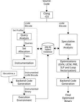
Our implementation is based on the LLVM Compiler Infrastructure. Figure 3.1 shows

Source Code Query Analysis Set Allocation Instrumentation Backend Code Generation Queries Sets Clang -O3 LLVM Bitcode Instrumented LLVM Bitcode Set Profiler ddp.db Sqlite3 Database Speculative Alias Analysis Optimizations (GVN, LICM, PRE,

SLP and Loop Vectorization) Backend Code Generation Execution Environment Instrumented Binary Final Optimized Binary LLVM Bitcode libruntime.a

Figure 3.1Work Flow for set profiling and feedback directed optimizations

the work-flow for profiling and feedback directed optimizations. We’ll focus on the portion

corresponding to Set Profiling here. The Set Profiling infrastructure is built as an LLVM tool

3.1. SET IMPLEMENTATION CHAPTER 3. INFRASTRUCTURE AND EVALUATION

analysis and set allocation are performed as an analysis pass. Each Load-Store pair (query)

which needs to be profiled is assigned a refID. As discussed earlier, at the very least all

refIDs corresponding to the same store instruction are grouped together and assigned a

set. More advanced grouping policies can be implemented. A subsequent instrumentation

pass generates the instrumentation code corresponding to all the queries and sets in the

program, function by function. In order to avoid the overhead of function calls, various variables are allocated on stack as needed, and the set operations are generated directly in

the IR. Finally module destructors are used to write the collected data to the SQLite database.

Library functions are used here to aid database access, since it is one time overhead at the

end of the program. Any storage mechanisms like files or databases can be chosen; we’ve

used SQLite database in order to simplify analysis of the data.

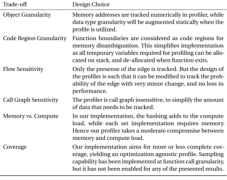
Table 3.1 presents various choices taken as per the design trade-offs explained in

chap-ter 1.

Set Implementation

Since the granularity of a 32-bit machine is 4 byte elements, we’ve used the same to build

set based bloom filters. Based on the desired size of the bit set, an array of 32-bit integers is

created. For example, to obtain a 512-bit set, an array of 16 elements can be created. Using

bit-wise operations, the index is also split into array index and bit index (to index inside 32

bits).

Signature Configurations

When implementing banked Signatures, the hashing work increases with each bank. In

order to reduce the hashing work, a single hash is computed for the whole 32-bit address,

using simple bit-wise operations. Lower two bits are discarded as most addresses are aligned on a 4 byte boundary. The next bits are used to index each bank. For example, with 512-bit

banks, the first bank will use bit 2-10 from the hashed address, the second bank will use bit

11-19 and so on. Since the hash is computed using the whole 32-bit address, information

for all the bits is utilized in the index, even though some bits of the hash are unused in

3.1. SET IMPLEMENTATION CHAPTER 3. INFRASTRUCTURE AND EVALUATION

Table 3.1Design choices taken in our implementation

Trade-off Design Choice

Object Granularity Memory addresses are tracked numerically in profiler, while data type granularity will be augmented statically when the profile is utilized.

Code Region Granularity Function boundaries are considered as code regions for memory disambiguation. This simplifies implementation as all temporary variables required for profiling can be allo-cated on stack, and de-alloallo-cated when function exits. Flow Sensitivity Only the presense of the edge is tracked. But the design of

the profiler is such that it can be modified to track the prob-ability of the edge with very minor change, and no loss in performance.

Call Graph Sensitivity The profiler is call graph insensitive, to simplify the amount of data that needs to be tracked.

Memory vs. Compute In our implementation, the hashing adds to the compute load, while each set implementation requires memory. Hence our profiler takes a moderate compromise between memory and compute load.

Coverage Our implementation aims for more or less complete cov-erage, yielding an optimization agnostic profile. Sampling capability has been implemented at function call granularity, but it has not been enabled for any of the presented results.

Table 3.2Signature Configurations

Signature Banks Bits/bank Index bits per bank Utilized bits of hash

1K 2 512 9 18

2K 2 1024 10 20

3K 3 1024 10 30

3.2. ACCURACY CHAPTER 3. INFRASTRUCTURE AND EVALUATION

exploring various options.

Accuracy

Same methodology as illustrated in[VT12]is used to evaluate the accuracy of the profiler. We use a fully accurate profiler as a comparison point.

Perfect Profiling

To evaluate the profiling accuracy, a perfect profiler is required, which has knowledge of

all the edges. Such a perfect profiler can be implemented using dynamic data structures.

The set based implementation is augmented with the STL sets in C++ [ISO14], to build a perfect profiler. STL sets allow perfect insertion and membership checks, but at the cost

of speed. Any perfect profiler has to use such dynamic data structures, which are slow to

allocate and traverse. So, this also serves as a reasonable performance comparison point.

Normalized Average Euclidean Distance

We use Normalized Average Euclidean Distance (NAED)[SS06]for our accuracy compar-isons. All the results of the profiler are placed into a vector, such that each dimension

in the vector represents a unique query (static data dependence edge). The value of this

dimension is the probability of the edge occurring as per the profiler under consideration. The probability is calculated by dividing the number of times that edge occurs, with the

number of times that code-region executes (normalization).

Once the data dependence vectors are obtained, a Euclidean distance is calculated i.e.

dis-tance between components along corresponding dimensions is calculated. Next, Average

Euclidean Distance is obtained by dividing the ED withs q r t(n)wheren is the length of the vector. This can be represented in Equation 3.1

N AE D = v tPn

i=1(p e r f e c ti−p r o f i l e ri)2

3.3. EXPERIMENTAL SETUP CHAPTER 3. INFRASTRUCTURE AND EVALUATION

Since each vector is a vector of probabilities ranging from 0 to 1, the final NAED will also

have a range of 0 to 1. This can be visualized with following examples. If a program has 100

queries, and the profiler predicts each query off by 20%, the final NAED would be 0.2. On

the other hand, if 20 of them were 100% wrong, the resulting NAED would be 0.447.

Experimental Setup

The performance evaluation of the instrumented binaries was done natively, using

equiva-lent nodes on a High Performance Computing systems. Each node sports a Intel EE5520

quad-core machine with two-way hyper-threading, paired with 24GB of memory,

run-ning a RHEL7 OS. In order to ensure that other jobs on the HPC systems do not affect the

performance evaluation, each job is executed with exclusive access to the machine.

Both integer and floating-point benchmarks from SPEC2000 and SPEC2006 benchmark

suites are used to study accuracy as well as performance. Only the benchmarks written in

C and C++are selected because LLVM/Clang frontend supports GNU toolkit compatible compilation for these two languages. Some benchmarks which exhibit too long runtimes

with perfect profiling are omitted. LLVM version 3.6.2 is used for all the evaluation.

Performance is measured as the slowdown in comparison to the -O3 optimized

non-instrumented code.

0 0.1 0.2 0.3 0.4 0.5 0.6 0.7 0.8

1k 2k 3k 8k

N

A

E

D

0.2

0.16

0.1 0.09

3.4. EVALUATION CHAPTER 3. INFRASTRUCTURE AND EVALUATION

Figure 3.2 shows the accuracy of the profiler for different benchmarks, along with the

arithmetic mean. The benchmark-configuration pairs with no bars imply a perfect

accu-racy of NAED=0. The signature based profiler provides moderate accuracy – a NAED of 0.2 with 1K bits per signature and 0.09 with 8K bits per signature on average. The size of the

signature presents the expected trend with bloom filters i.e. accuracy improves with the size

of the bloom filter. But the accuracy does not linearly increase with increased size; it rather improves suddenly depending on the benchmark. This is because the address patterns

input to the sets do not follow a random distribution, but depend on the program accesses.

Because 3K configuration uses an extra bank (and a hash) above 8K configuration,

some-times it provides higher accuracy. Depending on the sensitivity of the benchmark to the

higher order bits of the address, 3K can be more effective, as observed on 183.equake and

300.twolf. Though the average NAED is quite low, not all benchmarks have good accuracy

individually. Benchmarks like 188.ammp show a very poor or inaccurate profile at 1K; even

with the 8K configuration the NAED is 0.5, which is too large to be useful. For the

bench-marks 179.art, 181.mcf, 183.equake the inaccuracy is quite high when using low signature sizes, but it improves to some extent with higher signature sizes. For other benchmarks as

0 10 20 30 40 50 60 10 3. 66 28 3. 75 96 .6 5 91 .5 5 20 1. 07 12 5. 59 55 1. 03 84 .3 9 69 .1 9 59 .9 4 perfect 8k 3k 2k 1k S lo w d o w n 24.98 7.18 7.88 6 5.97

3.4. EVALUATION CHAPTER 3. INFRASTRUCTURE AND EVALUATION

Figure 3.3 shows the performance of various configurations with respect to the perfect

profiler, along with the geometric mean across all benchmarks. The Y axis presents the

factor of slowdown compared to the uninstrumented code. The performance overhead

of signature profiling is much lower than perfect profiling, for most of the benchmarks

– on average it has a 7x runtime while the perfect profiler has a 24x runtime. In some

cases like 253.perlbmk the performance overhead of signature based profiler is almost at par or even worse than perfect signature. A possible explanation for this is that these

benchmarks have small functions being called repeatedly, which results in initialization

costs to accumulate. Even simple operations like clearing the memory initially add up. The

perfect set implementation on the other hand allocates memory on-the-fly and hence does

not have high initialization cost. A comparison with just the memory clearing disabled in

the signatures, confirms this intuition. The generated profile however, would be garbage

and hence it is not presented as a point of comparison. The performance is highly sensitive

to the number of banks, as the amount of computation required per set operation increases

with each bank. This is visible as the overhead of 3K configuration is higher than other configurations, even 8K, due to its extra bank. The overhead does increase from 1K to 8K,

but the increase is not very significant. As the accuracy gains are much more significant

CHAPTER

4

HOW TO IMPROVE

Set based profiling achieves fast profiling with reasonable accuracy as compared to perfect

profiling. But what can be improved to achieve lower performance overhead and improve

the accuracy of the generated profile?

What to profile

One strategy to select queries is to profile every load-store edge which can’t be statically

proven. This allows the profiler to be optimization agnostic – any speculative optimizations can use this profile. This is the current policy used to select queries.

The other extreme is to build a list of edges that cause optimizations to give up, and

then only profile these edges. This strategy reduces the amount of information that needs

to be captured by the profiler, reducing its overhead. Though this may seem like a good

4.2. SET REPRESENTATION CHAPTER 4. HOW TO IMPROVE

fashion, where they give up as soon as a possible dependence is found. Even if that edge

is probabilistically dis-proven, there’s a high chance that there are more edges which will

block the optimization, and we have not profiled them yet. Moreover, this strategy makes

the obtained profile usable only with the optimization under consideration.

A reasonable middle ground would be to profile only the useful information, without

losing the generality of the profile. Many edges in the programs are relatively easy to predict statically, even though the predictions do not meet the strict correctness policy of compilers.

This information can be leveraged, to avoid profiling these edges and reduce the profiling

overhead, while still maintaining profile generality and completeness. Next chapter will

introduce few such heuristics to prune the query list for the profiler.

Set Representation

This is one of the most critical pieces for the profiler, as it directly controls the accuracy as

well as the performance per query. Bloom filters provide a relatively lightweight mechanism to capture the memory locations access, but can this information be represented in any

other form?

Subsequent chapters will introduce a simple yet effective range mechanism to represent

sets. Further this range mechanism will be combined with bloom filters to obtain high

CHAPTER

5

HEURISTIC PRUNING

The compilers and the Alias Analysis passes operate on a strict correctness principle, which

makes them pessimistic in many cases. Though a particular program pattern might be easy

to predict in most cases, due to some corner cases, it cannot be leveraged. Profilers on the

other hand are inherently probabilistic. And each memory operation being profiled can

add to the profiling overhead. Furthermore, since we are using probabilistic signatures to

profile each query, any information obtained from the profiler, can possibly be inaccurate,

depending on the population of the sets. Such program patterns available statically, can be

leveraged to predict dependence relations. And because these patterns are quite simple, they can be predicted more accurately as compared to the profile obtained from a probabilistic

profiler. In this chapter, some heuristics to prune the number of queries are proposed and

evaluated against the perfect profiler. All the code examples presented are written in LLVM

5.1. HEURISTICS CHAPTER 5. HEURISTIC PRUNING

Heuristics

Constant Data Space

An alias analysis pass being conservative, treats an unknown address as a possible conflict

with any other address. But in any correctly designed program, a load which is accessing a

constant memory space will never conflict with a store.

Code Snippet 5.1Constant Data Space Heuristic

1 @a = i n t e r n a l constant [5 x i 3 2] [i 3 2 1 , i 3 2 2 , i 3 2 3 , i 3 2 4 , i 3 2 5], a l i g n 16

2

3 d e f i n e i 3 2 @_Z6squarei ( i 3 2 %num) #2 { 4 . . .

5 %5 = g e t e l e m e n t p t r inbounds [5 x i 3 2]∗ @a , i 3 2 0 , i 6 4 %4 6 %6 = load i 3 2_∗ %5, a l i g n 4

7 . . .

8 s t o r e i 3 2 %6, i 3 2_∗ %unknown , a l i g n 4 9 . . .

10 }

Code Snippet 5.1 presents an example of such code pattern. The “load” instruction is

accessing a truth table which resides in a constant data space, while the memory location

accessed by the store is unknown. The only situation where this load and store can conflict,

is when the store tries to write to constant data space, in which case, program will crash due to illegal memory access. So, the profiler can avoid instrumenting all queries which

exhibit this pattern.

Structure Type Mismatch

Different structures in memory should never conflict. Even if the actual address of a

struc-ture cannot be traced, as long as they are different strucstruc-tures, they should never conflict.

5.1. HEURISTICS CHAPTER 5. HEURISTIC PRUNING

Code Snippet 5.2Structure Base Type Mismatch

1 %s t r u c t . i d l = type { i32 , double , i 6 4 }

2 %s t r u c t . uuuuu = type { i32 , i32 , i32 , i32 , i 3 2 } 3

4 d e f i n e i 3 2 @test ( i n t ) ( i 3 2 %x ) #0 { 5 . . .

6 %6 = g e t e l e m e n t p t r inbounds %s t r u c t . i d l_∗ %5, i 3 2 0 , i 3 2 0 7 s t o r e i 3 2 %4, i 3 2_∗ %6, a l i g n 4

8 . . .

9 %16 = g e t e l e m e n t p t r inbounds %s t r u c t . uuuuu_∗ %15, i 3 2 0 , i 3 2 1 10 %17 = load i 3 2_∗ %16, a l i g n 4

11 . . . 12 }

a member of the structure “%struct.idl”, while the load instruction is trying to access a

member of the structure “%struct.uuuuu”. Even though the base address of both these

structures (%5 and %15 respectively) are unknown statically, as they are different structure

types, they’ll be different locations in memory. Subsequently, the addresses accessing their

elements (%6 and %16 respectively) should be different. In LLVM IR, this is easy to track

since GetElementPtr are the only instructions which can be used to index into structures in

memory.

In most cases, this will be true, but in some corner cases this will not be true:

1. Nested Structures: In case of nested structure, the first element of the inner structure,

and the address of an inner structure as accessed from outer structure will have the

same address, even though they have different base structure types.

2. Casting: In case of equivalent structures that are casted from one type to the other,

two different structure base types may refer to the same memory location.

But as presented in the evaluation of the heuristics, such occurrences are not very common.

5.1. HEURISTICS CHAPTER 5. HEURISTIC PRUNING

Structure Index Mismatch

Different elements of any given structure should never conflict with each other, whether

they are part of the same instance or another.

Code Snippet 5.3Structure Index Mismatch

1 %s t r u c t . xyz = type { i32 , i32 , i 3 2 } 2

3 d e f i n e i 3 2 @test ( i n t ) ( i 3 2 %x ) #0 { 4 . . .

5 %6 = g e t e l e m e n t p t r inbounds %s t r u c t . xyz_∗ %5, i 3 2 0 , i 3 2 2 6 s t o r e i 3 2 %4, i 3 2∗ %6, a l i g n 4

7 . . .

8 %16 = g e t e l e m e n t p t r inbounds %s t r u c t . xyz_∗ %15, i 3 2 0 , i 3 2 1 9 %17 = load i 3 2_∗ %16, a l i g n 4

10 . . . 11 }

Code Snippet 5.3 shows one such scenario. The “%struct.xyz” is a structure with three

elements. The store instruction accesses the last element, while the load instructions

accesses the second element of the structure. Irrespective of whether both of the elements

are a part of the same instance of that structure or a different instance, they should not

conflict.

One of the rare cases when this heuristic will not hold true is when a structure is used to

walk an array of elements. For example, a structure containing only 2 integer elements, is

used to walk an array of 1000 integers, where in each iteration, the array index is incremented

only by one integer, and casted to the structure. But this is a very rare case situation.

Local Variables vs. Unknown Aggregates

Programs allocate local variables (simple data types) on the stack, specific to functions or

regions of code. These variables are cannot conflict with any aggregates, even if unknown,

5.1. HEURISTICS CHAPTER 5. HEURISTIC PRUNING

Code Snippet 5.4Local Variables vs. Unknown Aggregates

1 %s t r u c t . xyz = type { i32 , i32 , i 3 2 } 2

3 d e f i n e i 3 2 @test ( i n t ) ( i 3 2 %x ) #0 { 4 . . .

5 %3 = a l l o c a i32 , a l i g n 4 6 . . .

7 %6 = g e t e l e m e n t p t r inbounds %s t r u c t . xyz_∗ %5, i 3 2 0 , i 3 2 2 8 s t o r e i 3 2 %4, i 3 2_∗ %6, a l i g n 4

9 . . . 10

11 %17 = load i 3 2_∗ %3, a l i g n 4 12 . . .

13 }

Code Snippet 5.4 illustrates an example function. The load instruction can be traced back

to an alloca instruction, which allocates a variable on the stack. The store instruction on the other hand accesses an unknown memory location, but we know that it is indexing into an

aggregate of type “%struct.xyz”. This heuristic can be incorrect only when programmer is

relying on the order of the variables on the stack, or the program has an overflowing pointer,

which causes memory corruption. Various optimizations in compilers move variables

around, and sometimes even promote them to registers. So, such an access would be illegal

for a programmer to implement anyway.

Local Structures vs. Function Arguments

Programs also allocate data structures on stack, which are specific to functions or regions

of code. These data structures cannot conflict with the arguments passed through the

arguments of the function, since they are freshly allocated on the stack.

Code Snippet 5.5Local Structures vs. Function Arguments

5.1. HEURISTICS CHAPTER 5. HEURISTIC PRUNING

3 d e f i n e i 3 2 @test ( i n t ) (% s t r u c t . l i s t _ e l_∗ %x ) #0 { 4 . . .

5 %2 = a l l o c a %s t r u c t . l i s t _ e l , a l i g n 4 6 . . .

7 %6 = g e t e l e m e n t p t r inbounds %s t r u c t . l i s t _ e l∗ %x , i 3 2 0 , i 3 2 0 8 s t o r e i 3 2 %4, i 3 2_∗ %6, a l i g n 4

9 . . .

10 %next = g e t e l e m e n t p t r inbounds %s t r u c t . l i s t _ e l_∗ %2, i 3 2 0 , i 3 2 1

11 %17 = load %s t r u c t . l i s t _ e l_∗∗ %next , a l i g n 4 12 . . .

13 }

In Code Snippet 5.5, the load instruction (line number 11) is indexing into a local data

structure “%2”, and the address for the store (line number 8) can be traced back to a function

argument. These instructions will not conflict as an argument passed to the function will not conflict with the local stack. A situation where this heuristic can be incorrect is when

the caller function relies on specific memory layout of function’s local structures which

will be created in future, when the call instruction actually executes. Since optimizations

can move or promote these aggregates to individual elements, or even registers, this is an

illegal assumption. Note that the tracing is not done through a load instruction. Tracing is

performed only through pointer manipulation instructions like BitCast and GetElementPtr.

This heuristic differs from the previous one in the sense that previous one is restricted

to only simple data types, but in this heuristic even complex data types like aggregates can

be compared to function arguments.

Local Variables with No Pointers

Lastly, many of the local variables or structures allocated are only used as temporary storage

elements, specific to regions of code. No pointers are created to point at them i.e. no store

instructions store their addresses into the memory (at some other location). Since these

5.1. HEURISTICS CHAPTER 5. HEURISTIC PRUNING

structures will not conflict with other addresses.

Code Snippet 5.6Local Variables with No Pointers

1 %s t r u c t . l i s t _ e l = type { i32 , %s t r u c t . l i s t _ e l_∗ } 2

3 d e f i n e i 3 2 @test ( i n t ) (% s t r u c t . l i s t _ e l_∗ %x ) #0 { 4 . . .

5 %2 = a l l o c a %s t r u c t . l i s t _ e l , a l i g n 4 6 %3 = a l l o c a %s t r u c t . l i s t _ e l , a l i g n 4 7 . . .

8 %6 = g e t e l e m e n t p t r inbounds %s t r u c t . l i s t _ e l∗ %3, i 3 2 0 , i 3 2 1 9 s t o r e %s t r u c t . l i s t _ e l %x , %s t r u c t . l i s t _ e l_∗∗ %6, a l i g n 4

10 . . .

11 %next = g e t e l e m e n t p t r inbounds %s t r u c t . l i s t _ e l_∗ %2, i 3 2 0 , i 3 2 1

12 s t o r e %s t r u c t . l i s t _ e l %3, %s t r u c t . l i s t _ e l_∗∗ %next , a l i g n 4 13 . . .

14 %20 = load %s t r u c t . l i s t _ e l_∗ %unknown , a l i g n 4 15 . . .

16 }

In Code Snippet 5.6, let’s assume that all the uses of “%2” and “%3” are shown. The address “%2” is not used in a store instruction as a data operand; it is used only as the address

operand on line number 12 (traced through a GetElementPtr). So the query formed by the

store instruction on line number 12 and load instruction on line number 14, can never

form an edge. On the other hand, the address “%3” has been used as the data value in store

instructions. So, the query between the store on line number 9 and load on line number 14,

5.2. EVALUATION CHAPTER 5. HEURISTIC PRUNING

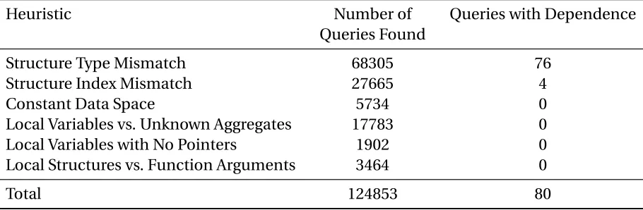
Table 5.1Queries detected by heuristics across all benchmarks

Heuristic Number of

Queries Found

Queries with Dependence

Structure Type Mismatch 68305 76

Structure Index Mismatch 27665 4

Constant Data Space 5734 0

Local Variables vs. Unknown Aggregates 17783 0

Local Variables with No Pointers 1902 0

Local Structures vs. Function Arguments 3464 0

Total 124853 80

Evaluation

These heuristics are not perfect and need to be evaluated for correctness. The perfect

profiler has the accurate data for all these edges, and can be used verify these heuristics.

Table 5.1 shows the number of queries detected by the heuristics, and the number of

actual dependences as per the perfect profiler. These are combined numbers for all the

benchmarks. Figure 5.1 shows the distribution of each heuristic for each benchmark. The

heuristics are applied in the same order as specified in the table, each query is counted only

for one of the heuristics. As we can observe, the number of statically predictable queries is quite significant. Different heuristics are prominent on different benchmarks. TheStructure

Type MismatchandStructure Index Mismatchheuristics are most commonly observed. The inaccuracy introduced due to the heuristics is negligibly small – only 0.06% edges

are incorrectly skipped. All other edges are correctly predicted, thus eliminating the need

to profile these edges.

The 4 dependence queries found for theStructure Index Mismatchheuristic occur in

176.gcc benchmark, which has a union containing packed data structures. So it is possible

that seemingly different indices might be pointing to the same address, misleading the

heuristic. Out of the 76 failed cases for theStructure Type Mismatchheuristic, 48 queries are

5.2. EVALUATION CHAPTER 5. HEURISTIC PRUNING

these benchmarks use casting among different structures which have the same or similar

type layout, thus triggering the heuristic wrongly. Nevertheless, such occurrences are also

very rare as visible from the table, and do not affect the accuracy significantly.

0 10 20 30 40 50 60 70 80 90

Structure Base Mismatch Structure Index Mismatch Constant Data Space Alloca vs. GEP Alloca with no Pointers Alloca vs. Arguments

%

Q

ue

rie

s

D

is

ca

rd

ed

0 0.1 0.2 0.3 0.4 0.5 0.6 0.7 0.8 0.9

1k 2k 3k 8k

N

A

E

D

0.2

0.16

0.2 0.11

Figure 5.2Accuracy observed with Signatures on only those queries which can be statically predicted with the heuristics.

5.2. EVALUATION CHAPTER 5. HEURISTIC PRUNING

Figure 5.2 shows the accuracy when these queries are profiled with bloom filter based

profilers. Bloom filters perform poorly when they are highly populated, and that’s most

likely the reason behind such inaccuracy. These queries contribute to overall inaccuracy of

the profiler, especially in benchmarks like 188.ammp and 179.art. Overall it is quite clear,

0 0.1 0.2 0.3 0.4 0.5 0.6

8k

8k+Heuristics

N

A

E

D

0.09 0.06

0 10 20 30 40 50 60 70 80 90

8K

8k+heuristics

S

lo

w

d

o

w

n

7.18 6.24

5.2. EVALUATION CHAPTER 5. HEURISTIC PRUNING

Figure 5.3 shows the impact of the heuristics on overall accuracy. On an average the

NAED(w.r.t perfect profiler) is reduced by 32% as compared to the 8K configuration, which

had best accuracy till now. On specific benchmarks like 188.ammp, the difference is drastic,

as the profiler goes from being completely unusable to reasonably accurate.

Figure 5.4 shows the performance of the profiler with and without the heuristics. Only 8K

configuration has been presented here for the sake of simplicity; other configurations show a similar trend. The performance overhead is reduced by roughly 10%. The reduction in

performance overhead is not very significant, given the large number of discarded queries

as shown in Figure 5.1. This is due to the fact that performance is affected by the amount of

queries removed from the critical region, and not just any queries.

CHAPTER

6

RANGE SETS AND HYBRID SETS

In most cases, the memory is allocated for variables in a consecutive fashion, either on

stack or heap. Furthermore, most of the memory operations operate on a small range of

memory. For example, the iterator in a loop typically walks over an array. Even when objects

are allocated on heap, they are allocated in large chunks, or at least on nearby chunks. This

information can be represented in the form of a range.

Range Set

A range set is simply a set which keeps track of the range of addresses accessed by a given

instruction. The bloom filters try to hash a full 32 bit address space into a small set of bits.

In reality, the actual range of addresses accessed by any instruction in a single instance

of dynamic region of code, is usually very limited. The range set leverages this fact to

6.1. RANGE SET CHAPTER 6. RANGE SETS AND HYBRID SETS

technique is reminiscent of previous work in debugging[HL02; Zho04b; DZ09; Zho04a]. It is implemented using two variables which keep track of the minimum and maximum value

of the elements inserted into the set. Figure 6.1 shows the insertions into a range set during

Min = 0xABCD00

Max = 0xABCD00

Range Set

Min = 0xABCD00

Max = 0xABCD04

Range Set

Min = 0xABCD00 Max = 0xABCD24

Range Set

Min = 0xABCD00 Max = 0xABCD24

Range Set

MembershipCheck ( 0xABCF00 ) = False

a) 1st _{Iteration b) 2}nd _Iteration

c) 10th _{Iteration d) Membership Check}

Figure 6.1Operation of the range set: “a)” to “c)” show insertion and “d)” shows membership check.

multiple iterations of a loop. Each insertion grows the range, if the address is outside the

6.2. HYBRID SET CHAPTER 6. RANGE SETS AND HYBRID SETS

minimum and maximum values.

This set cannot distinguish if any intermediate addresses have been accessed or not.

For example, in Figure 6.1 the address 0xABCD20 might not have been accessed at all, but a

membership check will be positive. This is the main source of inaccuracy in the range set.

The range set performs well with densely packed memory access pattern, but poorly with

sparse access patterns. This would be especially detrimental when distinguishing between elements of a structure, inside an array of structures. Inside a loop, the range set will grow

up to the size of the whole array. Any memory operations on different elements of the

structure will alias with each other as they’ll have more or less the same range. This is where

Structure Index Mismatchheuristic will help, as it will be able to statically differentiate between different elements of the structure. This difference is visible on the 188.ammp

benchmark significantly as the NAED for the range set reduces from 0.56 to 0.15 with the

heuristics applied.

Hybrid Set

Bloom filters provide a simple way to compress a very large address space into small bits,

with the down side of aliasing. Because of this, memory accesses to completely different

regions like stack and heap can also alias to the same bits, resulting in the false edges. Range

set on the other hand provides a very accurate mechanism to separate different memory

regions like stack and heap, or even chunks of memory allocated at different places in

the same region. But it cannot distinguish between sparse memory accesses in that range.

Hybrid set combines these mechanisms with following set operations.

1. Insertion: Any new entry updates the minimum and maximum, as well as the

corre-sponding bits in the bloom filter.

2. Membership Check: First the address is checked whether it falls in the minimum or

maximum range. Only if it does fall in the range, it is checked for membership inside

the bloom filter.

Since the bloom filter check is not executed all the time, the performance overhead should

6.3. EVALUATION CHAPTER 6. RANGE SETS AND HYBRID SETS

to the combined effect, the accuracy should be at least as much as the best of both, or

sometimes even better than both of them.

Evaluation

Same methodology is used for evaluation, as explained in chapter 3. For the sake of

com-parison simplicity, only the 8K signature configuration is compared. Also, all the heuristics

0.00 0.05 0.10 0.15 0.20 0.25

8k range hyb-8k

N

A

E

D

0.063 0.057

0.04

0 10 20 30 40 50 60 70 80 90

8k range hyb-8k

S

lo

w

d

o

w

n

6.24 5.94

3.46

6.3. EVALUATION CHAPTER 6. RANGE SETS AND HYBRID SETS

Figure 6.2 shows the comparison of range and hybrid sets. Range Set provides us very

good accuracy, much better than one would expect from such a simple mechanism. The

heuristics help in reducing the queries which will hit the holes in range set, improving it’s

accuracy. Many of the benchmarks like 401.bzip2, 433.milc and 473.astar show an

accu-racy much better than bloom filter, sometimes even near perfect. On others like 164.gzip,

183.equake, 188.ammp, 300.twolf, range set shows poorer accuracy in comparison to bloom filters. This suggests that both these mechanisms are suited for different set of memory

patters. The hybrid configuration combines the two, yielding best of the two techniques.

It is more accurate than both the techniques individually, and provides the best accuracy

observed so far, across all benchmarks.

The performance overhead of both the techniques is shown in Figure 6.3. Due to its

sim-plicity, the performance overhead of the range set is the least. Notably, even though hybrid

has to do additional work, it has less performance overhead than an equivalent bloom filter

configuration, except a few benchmarks. This is because most of the membership checks

fail at the range check itself, short circuiting all the work for hashing and checking the bloom filter. The overhead saved due to this, absorbs any additional overhead in insertion

and membership checks in case of actual dependencies, yielding better performance.

On an average, hybrid gives us roughly 5% lower performance overhead, and 38% more