Optimal Controller Design for Linear Inverted Pendulum and Double Inverted Pendulum System

(1)

ISSN(Online): 2320-9801

ISSN (Print): 2320-9798

International Journal of Innovative Research in Computer

and Communication Engineering

(An ISO 3297: 2007 Certified Organization)

Vol. 3, Issue 7, July 2015

Optimal Controller Design for Linear

Inverted Pendulum and Double Inverted

Pendulum System

Manaswita Sharma, Dr.Mrinal Buragohain

M.E Student, Dept. of Electrical Engineering, Jorhat Engineering College, Dibrugarh University, Assam, India

Associate Professor, Dept. of Electrical Engineering, Jorhat Engineering College,Dibrugarh University, Assam, India

ABSTRACT: The inverted pendulum system findsit’s most widespread application in the study of control engineering. This paper focused on modelling and performance analysis of linear inverted pendulum and double inverted pendulum system. A comparative study of the time specification performance of both the systems are shown using Linear Quadratic Regulator (LQR) controller. Two control methods are used in this paper, Linear Quadratic Regulator (LQR) and Linear Quadratic Gaussian (LQG) controller for linear inverted pendulum system. Simulation is done using Matlab software.

KEYWORDS:Inverted pendulum; double inverted pendulum; LQR; LQG; Kalman filter.

I. INTRODUCTION

The most commonly used systems in the research work in order to study various control theory such as nonlinear problems, robustness, ability and tracking problem are linear inverted pendulum and double inverted pendulum system. Therefore, these two systems have been the cosmic attention in control system based research field.

The inverted pendulum is an intrinsically unstable system with remarkably nonlinear dynamics. Being an intrinsically unstable system, the inverted pendulum is among the most difficult system and is one of the most important scholastic problems. The double inverted pendulum is also a very good system which is used widely in the field of control theory.

In the design of modern control system, optimal control theory is playing an increasingly vital role, whose main objective is to determine control signals that will cause a process (plant) to satisfy some physical constraints and at the same time maximize or minimize a chosen performance criterion. The designed approach used in this paper is the Linear Quadratic Regulator (LQR) controller for linear inverted pendulum system and double inverted pendulum system. Linear Quadratic Gaussian (LQG) controller is a combination of LQR designed with that of a Kalman Filter. In this paper LQG controller is used only for linear inverted pendulum system.

II. RELATED WORK

A.

.

Mathematical model of linear inverted pendulum

The mathematical model of linear inverted pendulum is being established by the method of mechanical analysis and it is given as follows:

Isolation force analysis for the cart and the rod is shown in the figure 2 and the figure 3.

Here, the control input is the force F. The outputs are the angular position of the pendulum ɵ (theta) and the horizontal position of the cart x.

(2)

ISSN(Online): 2320-9801

ISSN (Print): 2320-9798

International Journal of Innovative Research in Computer

and Communication Engineering

ẍ= ∑ = (F-N-b ̇)………(1)

ɵ̈= ∑ = (-NLcosɵ-PLsinɵ)……….(2)

Figure1: Schematic diagram of linear inverted pendulum Figure2: Isolation force analysis of the cart

Figure3: Isolation force analysis of the rod

In the inverted pendulum system, the interaction forces N and P were solved algebraically as: =˃N= m ̈ …… (3)

=˃P=m ( ̈ +g)… (4)

However, the position coordinates and are exact functions of ɵ.

̈ = ̈-Lɵ̇ sinɵ+L ɵ̈ cosɵ….. (5)

̈ =Lɵ̇ cosɵ+Lɵ̈sinɵ…….. (6) From equation(3),(4),(5) and (6),

N=m( ̈-Lɵ̇ sinɵ+L ɵ̈ cosɵ)………..(7) P=m( ɵ̇ cosɵ+Lɵ̈sinɵ+g)………..(8)

Summing the forces in the free body diagram of the cart in the horizontal direction, we get the following equation of motion:

Mẍ+ ̇+N=F

=˃(M+m)ẍ +b ̇ +mLɵ̈ cosɵ-mLɵ̇ sinɵ=F……….(9) Again we can write,

Psinɵ+Ncosɵ-mgsinɵ=mLɵ̈+mẍcosɵ………..(9)

To get rid of P and N terms in the equation above, we take the sum of the moments about the centroid of the pendulum which is as follows:

-PLsinɵ-NLcosɵ=Iɵ̈ ………..(10) Let us assume,

cosɵ=cos(π+φ)≈-1,sinɵ=sin(π+φ)≈-φ, ɵ̇ = ̇ ≈0

Now,we can write,

=˃ (I+ m ) ̈-mgLφ=mLẍ……….. (11)

F is replaced by u in equation (17) and considering the assumed conditions, we get, (M+m)ẍ+b ̇-mL ̈=u……….(12)

(3)

ISSN(Online): 2320-9801

ISSN (Print): 2320-9798

International Journal of Innovative Research in Computer

and Communication Engineering

=˃ ( )

( )= ( ) ( )

Meanwhile:

P=[(M+m)(I+mL2)-(mL)2]

By the principles of modern control theory, and then substituted the inverted pendulum system parameters which is designed into the state space equationis given by

Here,

M is the mass of the cart taken as 0.5kgs m is the mass of the pendulum taken as 0.2kgs

Lisdistance from the pivot to mass centre of the pendulumtaken as 0.4m G is the gravitation constant taken as 9.8m/

B .Mathematical model of double inverted pendulum

In order to perform any research work on any system, the first and foremost thing is to know about the system dynamics. The dynamics of the double inverted pendulum can be explained using a series of differential equations called the equations of motion ruling over the double inverted pendulum response to the applied force. The double inverted pendulum is shown in the figure(4) below:

The dynamics of double inverted pendulum can be found by Lagrange equation, which is given as: (

̇)- =0; i=0, 1, 2…n………..(13)

where L = T - V is a Lagrangian, Q is a vector of generalized forces (or moments) acting in the direction of generalized coordinates q and not accounted for in formulation of kinetic energy T and potential energy V.

The first pendulumkinetic energy is equal to the sum of the horizontal, vertical and rotational energy of pendulum.

Figure4: Schematic diagram of double inverted pendulum

xo=[₀]

x1=[

+ ɵ

ɵ ]

x2=[

+ ɵ + ɵ

ɵ + ɵ ]

(4)

ISSN(Online): 2320-9801

ISSN (Print): 2320-9798

International Journal of Innovative Research in Computer

and Communication Engineering

=>T= (m0+m1+m2) ̇ + (m1 +m2 + )ɵ̇ + (m2 + )ɵ̇ +

(m1l1+m2l1) ̇ɵ̇ ɵ +m2l2 ̇ɵ̇ ɵ2+m2l2l1cos(ɵ1-ɵ2)ɵ̇ ɵ̇ ……..(14)

The potential energy of the system is obtained separately for three parts of the system. The cart potential energy is zero and the potential energy for the two pendulumsis obtained. The total potential energy of the system is given by:

V=V0+V1+V2

=˃V=(m1l1+m2l1)cosɵ1+m2l2gcosɵ2……..(15)

Putting the (2) and the (3) equations in the Lagrange equation we have:

L= ( 0+m1+m2) ̇ + (m1 + 2 + 1)ɵ̇ + ( 2 + 2)ɵ̇ +(m1l1+m2l1) ̇ɵ̇ ɵ1+m2l2 ̇ɵ̇ ɵ2+m2l1cos(ɵ1

-ɵ2)ɵ̇ ɵ̇ -(m1l1+m2l1)gcosɵ − 2l2g cosɵ ………..(16)

Differentiating the Lagrangian by q and ̇ yields Lagrange equation (13) as: (

̇) - =u……… (17)

( _ɵ̇ ) - _ɵ =0……….. (18)

( _ɵ̇ ) - _ɵ =0………. (19) 0r in more detailed:

(m1 + 2 + )ɵ̈ + ( + ) ̈ ɵ + cos(ɵ −ɵ )ɵ̈ + sin(ɵ −ɵ )ɵ̇ −( +

) ɵ = 0……….(19)

( + )ɵ̈ + ɵ ̈+ cos(ɵ −ɵ )ɵ̈ − sin(ɵ −ɵ )ɵ̇ − ɵ =0……….. (20)

It is assumed that,

a0=m0+m1+m2; a1=m1l1+m2l2; a2=m1 + + ; a3=m2l2; a4=m2l1l2; a5=m2 + ; a6=(m1l1+m2l1)g;a7=m2l2g

As the controller can work only with the linear function so we need to linearized the above set of equation about ɵ1=ɵ2=0, sinɵ1=φ1, sinɵ2=φ2 and sin(ɵ −ɵ ) =φ1 – φ2, cos (ɵ −ɵ ) = 1, and cosɵ1=1,cosɵ2=1 and ɵ̇ =ɵ̇ = 0

̈+ ̈ + ̈ = … … … . . (21)

̈+ ̈ + ̈ − = 0 … … … . . (22)

̈+ ̈ + ̈ − = 0 … … … . (23)

It is assumed that, x as the cart displacement, ̇as the displacement velocity, 1 the first pendulum angle and ɵ̇ its

angular velocity, 2 the second pendulum angle and ɵ̇ its angular velocity, all as the state variables of the double

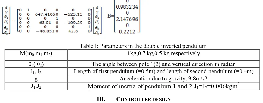
inverted pendulum system. The matrix A and B taken for double inverted pendulum is given as:

Table I: Parameters in the double inverted pendulum M(m0,m1,m2) 1kg,0.7 kg,0.5 kg respectively

θ1( θ2) The angle between pole 1(2) and vertical direction in radian

l1, l2 Length of first pendulum (=0.5m) and length of second pendulum (=0.4m)

g Acceleration due to gravity, 9.8m/s2

J1,J2 Moment of inertia of pendulum 1 and 2.J1=J2=0.006kgm 2

III. CONTROLLER DESIGN

A. DESIGN OF LINEAR QUADRATIC REGULATOR

(5)

ISSN(Online): 2320-9801

ISSN (Print): 2320-9798

International Journal of Innovative Research in Computer

and Communication Engineering

J= ∫ ( Qx+ Ru)dt

Where Q is the symmetric, positive semi-definite state weighting matrix, and R is the symmetric, positive definite control weighting matrix.

u (t)= -Kx(t)

Where K is the (m×n) control gain matrix given by K= R-1BTP

And P is the unique symmetric, positive semi-definite (n×n) solution of the algebraic Riccati equation. PA+ ATP – PBR-1BTP + Q=0

For linear inverted pendulum,

Firstly, Q and R is chosen as [100 0 0 0;0 1 0 0;0 0 100 0;0 0 0 1] and 1 respectively. Therefore, K= [1 4.8832 33.7437 20.6167].Secondly Q and R is chosen as [1000 0 0 0;0 1 0 0;0 0 1000 0;0 0 0 1] and R=0.1 respectively and K is found to be K= [100 74.4412 81.0153 -23.5443]

For double inverted pendulum, Firstly, Q and R is chosen as [100 0 0 0 0 0;0 1 0 0 0 0;0 0 100 0 0 0;0 0 0 1 0 0;0 0 0 0 100 0;0 0 0 0 0 1] and 1 respectively. Secondly, Q and R is chosen as [1000 0 0 0 0 0;0 1 0 0 0 0;0 0 1000 0 0 0;0 0 0 1 0 0;0 0 0 0 1000 0;0 0 0 0 0 1] and 0.1 respectively. The block diagram of LQR controller is shown in figure(5)

Figure5: Block diagram of LQR controller

B. DESIGN OF LINEAR QUADRATIC GAUSSIAN CONTROLLER

Kalman Filter

In the state space model used in the design of LQR, it was seen that the measurements y=Cx were assumed to be noise free. But practically it is not the usual case. Other unknown inputs yielding the state equations to be on the general stochastic state space form.

̇(t) = A(t)x(t) + B(t)u(t) + F(t)v(t)………..(24)

y(t) = C(t)x(t) + D(t)u(t) + z(t)………..(25) Here,

x is the state of the system; y is the measured output; u is the known input of the system;A, B,C are matrices that give value to their related system.

v(t) is process noise vector which arises due to modelling errors such as neglecting non-linear or higher frequency dynamics. And, z(t) is measurement noise vector .Both noises are assumed to be white noise.

The Kalman filter minimizes a statistical measure of the estimation error: e0 (t)= x(t) - x0(t)

Where, e0 (t)is the estimated state vector.

The state equation of the Kalman Filter is that of a time varying observer and can be written as follow: x0( t) = A( t)x0( t )+B( t )u( t) +L( t)[ y( t) –C( t) x0( t )-D (t )u (t)]

Where, L (t )is the gain matrix of the Kalman Filter (also called the optimal observer gain matrix). The optimal Kalman Filter gain can be computed as:

L0 (t) = Re0(t, t) CT( t) z-1( t)

Where, Re0(t, t)is the optimal covariance matrix satisfying the following Matrix Riccati equation.

dRe (t, t) / dt = A( t) Re0( t, t )+Re0( t, t )AT( t )-Re0( t, t) CT( t )z-1( t )C( t )Re0( t, t )+F( t )V(t)FT (t)

Here,steady state Kalman Filter is used, i.e. the Kalman Filter for which the covariancematrix converges to constant in the limit t →∞. In such a case, the following Algebraic Riccati Equationresults for the optimal covariance matrix, Re0

0 = Are0 +Re0 AT –Re0 CT z-1 CRe0 + FVFT

(6)

ISSN(Online): 2320-9801

ISSN (Print): 2320-9798

International Journal of Innovative Research in Computer

and Communication Engineering

Figure6: Block diagram of Kalman filter Figure7:Block diagram of LQG

LQG controller

LQG is a type of compensator. LQG, it is a combination of Linear Quadratic Regulator (LQR) designed with that of Kalman Filter. Here LQR is a linear regulator that minimized a Quadratic Objective Function, which includes transient, terminal, and control penalties. Kalman Filter is an optimal observer for multi output plant in the presence of process and measurement noise, modelled as white noise. The block diagram of LQG regulator is shown in figure (7).The software is based upon the equation (26) in order to calculate the state estimates.

̇ (t)=[A-BK-LC-LDK]x0(t)+Ly(t)

u(t)=-Kx0(t)

Where K and L are Optimal Regulator gain and Kalman Filter gain matrices.

Since, the optimal LQR controller for linear inverted pendulum is already found for two cases changing values of Q and R, hence, the obtained feedback gain matrix K, is directly used in the LQG design. After determining the measurement and disturbance noise covariance matrix, the Matlab function Kalman was used to determine the optimal Kalman gain matrix L and covariance matrix P. The gain matrix L for inverted pendulum is found to be:

L= 0.9984 1.0570 1.0570 2.9455 0.3432 1.3591 0.4201 1.8187

IV. SIMULATION RESULTS

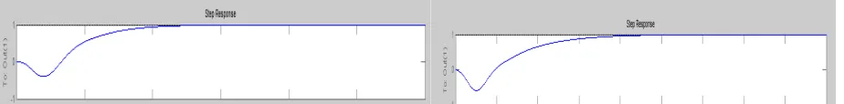
The simulation results using LQR with linear inverted pendulum and double inverted pendulum are shown below: Fig.8 and Fig.9 shows the step response of linear inverted pendulum taking two different values of Q and R as mentioned above.Similarly, fig.10, fig.12 and fig.14 shows the step response of the double inverted pendulum taking the first set of values for Q and R as mentioned above; fig.11, fig.13 and fig.15show the step response considering the secondset of values.

(7)

ISSN(Online): 2320-9801

ISSN (Print): 2320-9798

International Journal of Innovative Research in Computer

and Communication Engineering

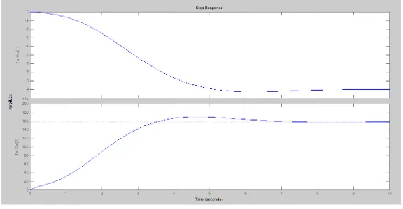
Fig 10. Step response of double inverted pendulum for position Fig 11. Step response of double inverted pendulum for position

Fig 12.Step response of double inverted pendulum ( ɵ) Fig 13.Step response of double inverted pendulum ( ɵ )

Fig14: Step response of double inverted pendulum (ɵ ) Fig15: Step response of double inverted pendulum (ɵ )

TableII.Characteristics of fig. (8)

Parameters Settling time (in seconds)

Rise time (in seconds)

x 3.9 1.64

̇ 4.35 0

ɵ 4.81 0

ɵ̇ 3.3 0

TableIII.Characteristics of fig. (9)

x 3.83 1.62

̇ 3.62 0

ɵ 4.85 0

ɵ̇ 2.72 0

Table II and Table III shows the settling time and rise time of linear single inverted pendulum with different values of Q and R on the application of LQR controller. From the above two tables, it can be concluded thatwhen the value of Q matrix increases and R decreases, settling time and rise time decreases.

TableIV.Characteristics of fig (10), fig. (12) and fig. (14)

x 2.37 1.06

ɵ1 3.08 0

(8)

ISSN(Online): 2320-9801

ISSN (Print): 2320-9798

International Journal of Innovative Research in Computer

and Communication Engineering

Table V.Characteristics of fig. (11), fig (13) fig (15)

x 2.15 1.07

ɵ1 2.36 0

ɵ2 2.91 0

Table IV and Table V shows the settling time and rise time of double inverted pendulum with different values of Q and R on the application of LQR controller.From the above two tables, it can be concluded that when the value of Q matrix increases and R decreases, settling time and rise time decreases.

The simulation results of LQG controller with inverted pendulum system is shown below in fig16.

Table VI.Characteristics of figure (16) Parameters Settling time

(in seconds)

Rise time (in Seconds)

Overshoot (in %)

x 6.96 3.07 2.66

ɵ 6.42 2.46 7.08

Table VI showsthe settling time and rise time of linear inverted pendulum on the application of LQG controller. Comparing with table II, it can be concluded that settling time and rise time of inverted pendulum increases when LQG Controller is applied.

Fig.16: step response of LQG with inverted pendulum

V. CONCLUSION

In this paper,the mathematical modeling of inverted pendulum and double inverted pendulum are shown. LQR and LQG are the types of control approach used in the pendulum systems. These design methods have been successful in meeting the stabilization goals for the two used systems. From the simulation results, it is concluded that the designed controllers are effective and feasible.

REFERENCES

1.Hongliang Hong,Haobin Dong,Lianghua He,Yongle Shi, YuanZhang, “Design and Simulation of LQR controller with the linear inverted pendulum”, 978-0-7695-4031-3/10 $26.00 © 2010 IEEE DOI 10.1109/iCECE.2010.178

(9)

ISSN(Online): 2320-9801

ISSN (Print): 2320-9798

International Journal of Innovative Research in Computer

and Communication Engineering

3. Solid high-pendulum system and automatic control experiments. Solid high-tech(Shenzhen)Co.,Ltd.,2002.8

5. Narinder Singh Bhangal, “Design and Performance of LQR and LQR based Fuzzy Controller for Double Inverted Pendulum System” ,©2013 Engineering and Technology Publishing doi: 10.12720/joig.1.3.143-146

6. Jiao-long Zhang, Wei Zhang, “LQR self-adjusting based control for the planar double inverted pendulum”,© 2011 Published by Elsevier B.V. Selection and/or peer-review under responsibility of ICAPIE Organization Committee.

7. Rachel Kalpa K., Madhu N. Belur, “ Singular LQR Control, Impulse-Free Interconnection and Optimal PDController Design”,2011 50th IEEE Conference on Decision and Control andEuropean Control Conference (CDC-ECC)Orlando, FL, USA, December 12-15, 2011

8.Ragnar Eide, Per Magne Egelid, Alexander Stamso, Hamid Reza Karimi, “LQG Control Design for Balancing an Inverted Pendulum Mobile Robot”,Intelligent Control and Automation,2011,2,160-166 doi:10.4236/ica.2011.22019 Published Online May 2011.