ABSTRACT
GANDHI, SHRUTI. Joint Virtual Machine Placement and Path Selection for Service Level Agreement based Resource Allocation in a Virtualized Datacenter Environment. (Under the direction of Ioannis Viniotis .)
In cloud computing environments multiple tenants share data center infrastructure compris-ing of compute, storage and data center network bandwidth. Currently, tenants pay for compute and storage resources using the pay-as-you-go approach, while intra datacenter network band-width is provided on a best-effort basis. The main problem with this approach employed by cloud providers is that, by guaranteeing resources and services over a best-effort intra datacenter network, an implicit network cost is added for tenants.
The problem becomes significant as intra datacenter network bandwidth incurs high perfor-mance variability due to its inherent shared nature, which in turn leads to variable perforperfor-mance for tenants’pay-as-you-go on-demand resources and services. Current cloud service level agree-ments (SLAs) do not guarantee intra datacenter network bandwidth, becoming inequitable to tenants.
© Copyright 2017 by Shruti Gandhi
Joint Virtual Machine Placement and Path Selection for Service Level Agreement based Resource Allocation in a Virtualized Datacenter Environment
by Shruti Gandhi
A thesis submitted to the Graduate Faculty of North Carolina State University
in partial fulfillment of the requirements for the Degree of
Master of Science
Computer Networking
Raleigh, North Carolina 2017
APPROVED BY:
Mihail Sichitiu Harilaos Perros
DEDICATION
BIOGRAPHY
ACKNOWLEDGEMENTS
I would like to thank my advisor for his invaluable guidance, his continuous faith and patience, bringing me back to the correct path whenever I wavered, and his ever beaming presence which in itself fills me with confidence and inspiration. I would also like to thank Anand sir for his brilliant insights and guidance.
TABLE OF CONTENTS
List of Tables . . . vii
List of Figures . . . .viii
Chapter 1 Introduction . . . 1
1.1 Motivation . . . 1
1.2 Main Contributions . . . 2
1.3 Literature Survey . . . 2
1.4 Roadmap . . . 5
Chapter 2 System Model . . . 6
2.1 Environment Model . . . 6
2.1.1 Background . . . 6
2.1.2 Environment Model Used . . . 9
2.2 System Service Level Agreement Model Formulation . . . 11
2.2.1 Current Cloud Service Level Agreements: A Comparison . . . 11
2.2.2 Proposed Cloud Service Level Agreement . . . 13
2.3 Problem Definition . . . 14
2.3.1 Identifying the Resources . . . 14
2.3.2 Identifying Performance Metrics . . . 16
2.3.3 Identifying Control Knobs . . . 17
2.3.4 Problem Statement . . . 20
2.4 Feedback Model as a Reference Model . . . 21
2.4.1 Goal . . . 21
2.4.2 System Under Management . . . 22
2.4.3 Monitoring . . . 22
2.4.4 Processing Measurements and Decide Actions . . . 22
Chapter 3 Algorithm Design and Key Questions Formulation. . . 23
3.1 Algorithm Design . . . 23
3.1.1 Assumptions . . . 23
3.1.2 Greedy Left First Algorithm . . . 24
3.1.3 Semi Random Algorithm . . . 24
3.1.4 Randomized Algorithm . . . 26
3.2 Key Questions . . . 26
3.2.1 Datacenter Designer’s Point of View . . . 26
3.2.2 Datacenter Administrator’s Point of View . . . 30
Chapter 4 Implementation and Performance Evaluation . . . 31
4.1 Experimental Methodology . . . 31
4.1.1 Deciding Input Parameters . . . 31
4.2 Experiments . . . 35
4.2.2 What Bandwidth Should I Buy for My Layers? . . . 41
4.2.3 How Many Servers Should I Buy? . . . 51
4.2.4 Placement of Rate-Limiters . . . 53
4.2.5 Measuring Compliance to Service Level Agreement . . . 54
4.2.6 Summary . . . 55
Chapter 5 Conclusion and Future Work . . . 56
5.1 Conclusion . . . 56
5.2 Future Work . . . 56
LIST OF TABLES
LIST OF FIGURES
Figure 2.1 Abstract Feedback Model as a Reference Model . . . 21
Figure 3.1 Generic Fat Tree Topology . . . 24
Figure 3.2 Greedy Left First Algorithm . . . 26
Figure 3.3 Semi Random Algorithm . . . 28
Figure 3.4 Randomized Algorithm . . . 29
Figure 4.1 Abstract topology fixed for the analysis . . . 33
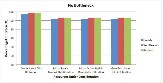
Figure 4.2 Percentage resource utilization when no bottleneck in the system. . . 36
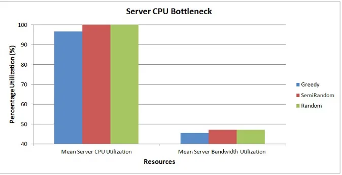
Figure 4.3 Percentage resource utilization when server CPU is bottleneck . . . 37
Figure 4.4 Percentage resource utilization when server bandwidth is bottleneck . . . 38
Figure 4.5 Percentage resource utilization when access uplink bandwidth is bottleneck 39 Figure 4.6 Percentage resource utilization when distribution uplink bandwidth is bottleneck . . . 39
Figure 4.7 Number of tenants served when the given resources are bottleneck or no system bottleneck . . . 40
Figure 4.8 Variation in Calculated and Experimental Server-Access Bisection Band-width with Total Number of Servers . . . 43
Figure 4.9 Variation of Bottleneck Utilization with Number of Tenants for Different Bottleneck Configurations, Bottleneck = Server Bandwidth . . . 44
Figure 4.10 Variation of Bottleneck Utilization with Number of Tenants for Differ-ent Bottleneck Configurations, Bottleneck = Access Bandwidth (19.99± 0.23Gbps) . . . 47
Figure 4.11 Tenants served with increasing per server uplink bandwidth . . . 48
Figure 4.12 Variation of SF Utilization with the given Topology Configurations . . . . 50
Figure 4.13 Variation of SF Utilization with Topology Configurations . . . 50
Figure 4.14 Variation in Calculated and Experimental Total virtual CPUs with Num-ber of Servers . . . 52
Chapter 1
Introduction
In this chapter we begin by motivating the problem, followed by providing the main contribu-tions of the study, and then provide a literature survey to summarize the previous work done in area of service level agreement based resource allocation, and finally provide a road-map for the chapters to follow.
1.1
Motivation
not only fundamental changes to the contemporary cloud service level agreements, but also requires unambiguous guidelines for designers and administrators to design and maintain cloud environments optimized for resource allocation based on such service level agreements.
1.2
Main Contributions
Major contributions of this study are the following:
Proposed a novel service level agreement to guarantee minimum compute and bandwidth to tenants
Designed and verified algorithms to implement the service level agreement
Answered based on experimental results, the key questions from a data center designer and administrator perspective, such as:
– How much bandwidth should I buy for my switch fabric?
– How many and what kind of servers should I buy for my data center?
1.3
Literature Survey
A Service Level Agreement between each business and service provider defines quality of service guarantees for a class of service [10]. The service provider gains revenues when these guarantees are satisfied, else incurs penalties, based on a predefined cost model. Service level agreement optimization aims to increase revenue for the service provider while the customers quality of service guarantees are met. Service level agreement optimization is very well studied area and is generally redefined as a resource allocation problem for a specific environment. This section analyzes the research work that has attempted to solve several service level agreement based resource allocation problems. For every analysis, upon identification of the resources in the system, knobs are identified for optimal allocation of resources. An algorithm is proposed for turning these knobs to maximize the values of the key performance indicators of the system.
and General Processor Sharing assignments (scheduling) by iteratively running the fixed point algorithms until convergence. A key contribution of this paper is the cost model which suggests that the service provider earns revenue if and only if per-class service level agreement is satisfied else the service provider is penalized. The authors define per-class service level agreement as a service level agreement which includes tail distribution of per class delays along with throughput and mean delays as a quality of service metric or key performance indicators.
In [16] the authors propose an service level agreement based on customer quality of service requirements for software as a service in a cloud computing environment. The resources under consideration are the virtual machines which are rearranged dynamically with changing cus-tomer demands. The authors hence focus on cuscus-tomer driven management from software as a service (SaaS) providers perspective instead of focusing on increasing profits for the infrastruc-ture as a service (IaaS). The knobs to allocate, initiate, rearrange or remove the virtual machines lie in the platform layer of software as a service structure. The authors propose a strategy to map customer requirements to infrastructure level parameters, and scheduling policy to find where and which virtual machine has to initiated, to incorporate virtual machine heterogeneity based on price, dynamic service initiation time and data transfer time. The authors borrow the base algorithm from Compiere ERP [16], and modify it into two algorithms the worst fit case and the best fit case. They quantify the result using the following key performance indi-cators total cost, number of initiated virtual machines and percentage service level agreement violations.
In [9] the authors propose a multi-dimensional resource allocation scheme for multi-tier ap-plications that incur large inter service communication in a cloud computing system to optimize the total profit gained from the service level agreement contracts and lost from operational cost. The resources under consideration are computational capacity, memory and network bandwidth of the servers in a cloud computing environment. In this paper the authors consider two classes of service level agreements gold class where response time is guaranteed and bronze class which uses utility function based on the response time, and propose a unified framework for handling both, hence service level agreement based resource allocation. The authors propose the follow-ing strategy to solve this resource allocation problem a heuristic called force directed resource assignment is used to find an initial solution to the problem where first clients and tiers are selected by rank, and then for each client of each tier resources are allocated. This is followed by a resource consolidation algorithm inspired by force directed search to replace clients and reassign the resources. The main contribution of the paper is the server consolidation technique using force directed search that results in maximal profits in the given multi tier environment. In [7], authors determine the need for federation of cloud infrastructure service providers and propose a system called InterCloud for seamless autonomic provisioning of services across different Cloud providers. This paper does not fall in the regular template for resource allocation, this is because it proposes a new system that supports dynamic workloads in cloud computing environment but does not specify a model for optimal service level agreements that are integral to the system.
In [6], the authors propose a management algorithm for dynamic allocation of virtual ma-chines to physical servers with the goal of minimizing the time averaged number of physical servers hosting the virtual machines to support a workload at a specified rate of service level agreement violations and reduce the rate of service level agreement violations for a fixed capac-ity. The authors break down the algorithm into three steps, namely measurement of historical data, forecast of the future demand followed by remapping of the virtual machines to physical machines. The resource under consideration is the CPU capacity of the physical machines.
are the knobs , while throughput and weighted average of response time have been used as key performance indicators for performance measurement.
In [17] the authors propose a resource allocation approach in an e-business running cluster computing environment that minimizes the total cost of each node’s computational power while satisfying the quality of service criteria defined in an service level agreement. The main contri-bution of the paper is that it analytically solves the problem under consideration by satisfying a set of four quality of service metrics or key performance indicators, namely percentile response time, cluster utilization, packet loss rate and cluster availability, and they do so by using a queuing network method. The authors take into consideration only computational cluster in a node as a resource, and ignore the storage station.
1.4
Roadmap
The thesis is organized in four chapters.
In Chapter 2, the system model is defined and the problem definition is formalized.
In Chapter 3, solution algorithms are designed for service level agreement optimization and key questions are formulated from a designer and administrator perspective
In Chapter 4, the proposed algorithms are validated and their performance compared. An experimental methodology is designed, and previously formulated key questions are answered.
Chapter 2
System Model
This section is divided into four parts, in the first part we discuss concepts that form neces-sary background, followed by formulation of the environment model that describes the system context, characteristics and key actors involved. In the second section, we compare service level agreements of contemporary cloud providers, and propose a novel service level agreement that meets their drawbacks. In the third section, the main problem being solved is formulated, and finally, in the fourth section, the problem is modeled using the abstract feedback model. The purpose of this section is for the reader to get an in-depth view into the problem being solved.
2.1
Environment Model
In this section we build the environment model used in this study. We start by explaining specific keywords that form the background of the study, we then fix the environment characteristics and describe our rationale in doing so.
2.1.1 Background
The environment in any study can be divided into two broad categories, the domain being studied, and actors working in that domain or affecting the behavior of the domain. The domain in consideration is a data center, and the actors are service providers, customers, designers and administrators. In this section we briefly describe the characteristics of the domain and the actors relevant to the study.
Data Center
The key characteristics of a data center are as
follows- Data Center Network: The switch fabric in a data center interconnects servers, stor-age devices through networking devices. The property of the switch fabric that allows this communication between different data center components to happen is the network bandwidth.
– Intra Datacenter Network and Inter Datacenter Network Bandwidth:The network bandwidth carried by the datacenter switch fabric in a given data center is called intra datacenter network bandwidth, and network bandwidth across geo-graphically distributed data centers is called inter-data center network bandwidth. – Uplink and Downlink Bandwidth: The network bandwidth in the switch fabric
that serves southbound data like user requests from the internet to a user assigned virtual machine in a data center server is called the down link bandwidth. The network bandwidth in the switch fabric that serves northbound data like internet facing responses to the user requests from the a virtual machine in a data center server is called the up link bandwidth.
– Bisection Bandwidth: Bisection bandwidth in a data center can be defined as the maximum bandwidth along a bisection of the network with minimum number of links. In a three tier topology, network bandwidth can be described using bisection bandwidths between any two adjacent tiers.
Data Center Topology: The way in which compute, storage and network resources inside a data center are interconnected forms a data center topology. The topology can change with changing network designer/administrator objectives. Numerous data center topologies have been proposed till date, the most used include, three tier, fat tree, leaf spine, VL2, portland, BCube, etc.
Data Center Traffic Characteristics:Traffic flowing inside a data center can be char-acterized in a number of ways, and more often than not these characteristics are not independent of each other.
– Data and Control Traffic: Traffic type can be broadly categorized into data and control type traffic, depending on whether it carries data or control type information. Data type traffic traverses the data path inside a switch/router and the control traffic traverses the control path.
– Control Traffic Types:Control traffic can be categorized into different types based on which control process inside the switch/router CPU it is intended for, for example, STP BPDUs, ARP traffic, OSPF packets, BGP traffic etc.
– Traffic Direction: Traffic can be identified as North-South, South-North, East-West, West-East type of traffic depending on the direction in which it traverses inside a data center. East-West traffic and vice-versa mainly refers to inter-virtual machine traffic.
– Frequency of Traffic: Traffic inside a data center can come in random bursts or at uniform rates, depends on the type of traffic in consideration.
Data Center Virtualization:A Virtualized Data Center is a data center where some or all of the hardware (e.g., servers, routers, switches, and links) are virtualized. Typically, a physical hardware is virtualized using software or firmware called hypervisor that divides the equipment into multiple isolated and independent virtual instances.
– Level of Virtualization:Depending on which physical hardware in a data center is being virtualized, the level of virtualization can be decided. Server level virtualization is achieved by virtualizing servers into virtual machines or containers. Network level virtualization is achieved by giving the physical network, or a one of the layers of the network stack, a property it doesn’t have, such as higher link bandwidth using ether-channel.
– Virtual Machine:Given a system, a physical server and a property of this physical server, the number of operating systems in the server. If we allow the server to have an ability to host more than one operating systems, it is said to be virtualized. This virtual abstraction of a physical server is called a virtual machine.
Actors
Cloud Provider: The entity that provides services, in a cloud computing environment is called the cloud provider.
Tenant: The entity that is the recipient of the service provided by a cloud provider is called a tenant. The term “tenant” is used to denote that the recipient is occupying space in terms of some resource(s) in the provider’s data center.
Datacenter Administrator:The entity responsible for outlining the management tasks, building test plans and finalizing the management tools to maintain a data center.
2.1.2 Environment Model Used
In this section we fix values for broad definitions given in the background.
Data Center
Data Center Network: Of the data center network characteristics mentioned in the background, intra datacenter traffic is assumed to be the only traffic type in the data center, similarly, video data type is assumed to be the primary data type flowing in the data center (see data center traffic characteristics in this section), up link bandwidth forms majority of the data center network bandwidth.
Data Center Topology: Current data centers follow to a great extend a common net-work architecture, known as the three-tier architecture [12]. At the bottom level, known as the server tier, each server connects to one (or two, for redundancy purposes) access switch. Each access switch connects to one (or two) switches at the distribution tier, and finally, each distribution switch connects with multiple switches at the core tier. The phys-ical topology in such three-tier architecture is a multi-rooted forest topology. [12].We use a version of this topology in our analysis. We compare scaling the topology by increasing switch FAN out capacities with increasing the number of switches in the topology to an-swer the key designer questions. In this study the focus is only on one topology. We may extend this work in the future to use more than one topology.
Data Center Traffic Characteristics:The traffic characteristics are fixed in this study, so as to not digress from the actual objective. The two traffic types consider in the data center are tenant requests for video streaming traffic and tenant response including the video. Since the video streaming data is much more bandwidth intensive than the tenant requests, the requests can safely be ignored.
– Data Traffic Type: Data traffic type in this study is limited to only video traffic. Recent studies have shown that video streaming is responsible for 25-40% of all Internet traffic [1, 11]. The two dominant sources for video streaming traffic in North America are Netflix and YouTube [1]. YouTube is also the most popular source of video streaming traffic in Europe and Latin America [1, 11].
– Traffic Direction:Since the traffic type being considered is only the video streaming data flowing from the data center servers to the users through internet via the core routers, the traffic direction is south-north, i.e. it uses up link bandwidth of the switch fabric bandwidth.
– Frequency of Traffic: Frequency of the tenant requests is uniform, in the sense that in the static algorithm considered the tenant requests are assumed to be already in queue at the core routers waiting to be served.
Data Center Virtualization:In this study data center virtualization has been limited to only server virtualization, i.e., the data center network or any other resource has not been virtualized.
– Level of Virtualization: Only server level virtualization is observed in the given environment. Server level virtualization is done to give the servers the property of hosting more than one independent machines called virtual machines. This is done to isolate all tenant requirements. Another key property of the given system is that no tenant is allowed to share servers at any time, i.e. at any time a tenant will be
allocated all requested compute through virtual CPU abstraction only on one server.
Actors
Cloud Provider:A cloud provider is the entity that provides the requested service to its tenants in a cloud computing environment while guaranteeing the proposed service level agreement service commitments.
Tenant:A tenant in this study is a customer who requests video streaming data by spec-ifying its requirements in the form of ‘Y’ Gflops CPU time, ‘X’ Mbps up link bandwidth. – Tenant Requirement Distribution: The tenant requirement distribution is as-sumed to be uniform random distribution. The random values are chosen between a given upper and lower bound.
– Tenant Uplink Bandwidth Requirement: The tenant up link bandwidth re-quirement is assumed to be the average bandwidth rere-quirement of more than one videos put forth in a single request by the tenant.
– Tenant Duration: A tenant once allocated resources inside the data center is as-sumed to occupy the resources forever.
Datacenter Administrator: A data center administrator in this context builds test plans, outlines management tasks and finalizes management tools to maintain a data center built using the finalized design blueprint generated by the DC Designer, all with the higher order objective of meeting the proposed service level agreement.
2.2
System Service Level Agreement Model Formulation
2.2.1 Current Cloud Service Level Agreements: A Comparison
In this section we compare the service level agreements for Infrastructure as a Service (IaaS) type services from IBM Softlayer [15], Amazon Web Services [2] and Microsoft Azure [4]. The criteria for comparison are (a)Service commitment (b)Service Credits offered by these cloud providers.
IBM Softlayer
IBM Softlayer uses a master service level agreement for all its infrastructure as a service offer-ings. On the first read the service level agreement seems better than other cloud service level agreements in terms of use of more granular time periods, but there are many self imposed ex-clusions, and intentionally vague keywords that makes it more favorable for the service provider than the customer. We explain this in detail with their offered service commitments and service credits.
Service Commitment: Softlayer claims to use reasonable efforts to provide a service level of 100% for the Public Network, Private Network, access to Customer Console and Redundant infrastructure, depending on the customer’s service. The keyword ’reasonable’ makes the statement vague, defining what is meant byreasonable efforts should be a part of the service level agreement, as it would make a stronger case for the customers deciding between cloud providers. Also, Softlayer doesn’t define the time period for which 100% of service level will be maintained.
Amazon Web Services EC2
Amazon Web Services EC2 service level agreement is for its Elastic Cloud Compute (EC2) service. Unlike IBM Softlayer, AWS fixes a measurement period over which it guarantees a minimum percentage of up time. But like Softlayer, it doesn’t define what is meant by keywords like reasonable effort. We explain this in detail with their offered service commitments and service credits.
Service Commitment: Like Softlayer, Amazon Web Services EC2 claims to use com-mercially reasonable efforts to make Amazon EC2 available to the customer for 99.95% of Monthly Up time Percentage (MUP). AWS service level agreement defines Monthly Up time Percentage to be minutes in monthminutes in month−minutes in region availability, and region unavailable as more than one availability zones in the same region where the customer is running their instances is unavailable to them. There is no commitment on the network availabil-ity to the customer to any public/private IP addresses within the same or different virtual networks.
Service Credit: The service level agreement offers 10% of customer fees for Monthly Up time Percentage between 99%,99.95%, and 30% for Monthly Up time Percentage less than 99%. This implies that there is no difference in the credit provided to the customer whether the customer receive service availability of 98.9% over the month or 0.1% over the month.
Microsoft Azure
Microsoft Azure defines its service level agreement specifically for virtual machines. Unlike IBM Softlayer, and like Amazon Web Services, Azure as well fixes a measurement period over which it guarantees a minimum percentage of up time. But unlike Softlayer and Amazon Web Services, it doesn’t use keywords like reasonable effort in its service commitment but instead promises service guarantee. We explain this in detail with their offered service commitments and service credits.
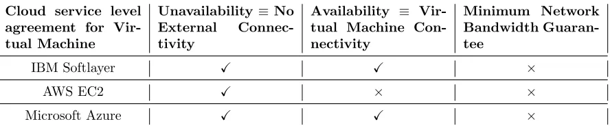
Table 2.1: Service Level Agreement Comparison
Cloud service level agreement for Vir-tual Machine
Unavailability≡No External Connec-tivity
Availability ≡ Vir-tual Machine Con-nectivity
Minimum Network Bandwidth Guaran-tee
IBM Softlayer X X ×
AWS EC2 X × ×
Microsoft Azure X X ×
Service Credit:The definition of Monthly Up time Percentage is the same for Microsoft Azure, but the service level agreement offers 10% of customer fees for Monthly Up time Percentage between 99%,99.95%, and 25% for Monthly Up time Percentage less than 99%, which is 5% less than Amazon Web Services EC2. So the argument of no difference in credit for any level of availability less than 99% remains same.
Summary
In this section we compared three service level agreement, and summarize our observations in a table as shown in table 2.1. In this table, the columns of unavailability ≡ no external connectivity implies whether the service level agreements defines the term unavailability in terms of external connectivity or not. Similarly if the term availability defined in the service level agreement includes virtual machine connectivity as a service commitment, i.e., connectivity to public/private network in same or different virtual network. Except Amazon Web Services EC2, both the service level agreements commit to this definition of availability. The common feature among all the service level agreements besides the service credit being returned to customer in terms of credit in their service account, is that all the service level agreements do not conform to crisp definitions of what exactly is being promised, this includes the intra datacenter network bandwidth, which even though customers are given a choice for the maximum speed of the up links/down links in the servers, there is no mention of the underlying data center network is provided on a best effort basis, and how that adds to the customer cost. As we can see that there is a lot of work needed to make the current service level agreements more equitable to the customers.
2.2.2 Proposed Cloud Service Level Agreement
an service level agreement that mitigates the drawbacks of the contemporary cloud service level agreements.
Guarantee ‘Y’ Gflops of CPU time and ‘X’ Mbps of up link bandwidth to each tenant in a virtual data center environment.
For all Y, X >0, where Y ≤Maximum available CPU capacity and X ≤Maximum available up link bandwidth.
2.3
Problem Definition
Our problem falls in the category of service level agreement based resource allocation in a virtualized data center network. The goal is to achieve the proposed service level agreement that guarantees Y Gflops of CPU time and X Mbps of up link bandwidth to each tenant in a virtualized data center environment.
2.3.1 Identifying the Resources
A resource is any component in a system that poses a contention for usage. In a data center, irrespective of it being virtualized or not, only three system components provide contention for usage. All tenants compete for CPU time for processing their requests, network bandwidth for transporting their requests and storage for storage space for their requests. In this section we briefly describe these resources, and identify resources of relevance to this study.
CPU Time
CPU time can be defined as the time spent by the CPU in processing a unit of traffic. It can be measured in Gflops, which can be defined as a unit of computing speed equal to 1×10⁹ floating point operations per second.
Why is CPU Time a Resource? In this study every tenant request is modeled as (CPU time, Bandwidth) tuple to comply with the proposed service level agreement. Con-sequently, every tenant request contends for CPU time, only then can it be served, hence a resource.
with the given processing capacity, it is required to efficiently utilize the server CPU time, and for the same reason CPU time is considered as a resource in this study.
CPU to Virtual CPU Mapping: In this study we assume that the server CPU time is divided into equal chunks and the hypervisor allocates one Gflop for each virtual CPU. Each virtual machine spawned in a server gets an integral number of virtual CPUs. The higher the number of virtual CPUs allocated to a virtual machine, higher is the underlying CPU time allocation which implies higher processing capacity.
Uplink Bandwidth
Link bandwidth expressed in bits per second (bps), denotes the maximum speed at which a link medium is able to carry information.
Why Bandwidth is a Resource? In this study every tenant request is modeled as (CPU time, Bandwidth) tuple to comply with the proposed service level agreement. Con-sequently, every tenant request contends for network bandwidth, only then can it be served, hence a resource.
Why Guarantee Network Bandwidth in Service Level Agreement?Current cloud service level agreements guarantee compute (dollars per unit time per virtual machine), storage (dollars per unit per GB), internet traffic (dollars per GB transferred), but none guarantee network bandwidth which becomes a crucial requirement for bandwidth inten-sive applications like High Performance Compute, High Quality Video, Voice or VoIP traffic. Since this study focuses specifically on video traffic, network bandwidth guarantee for a tenant becomes a key requirement for the service level agreement.
Storage
Storage expressed in bits is the memory space occupied by a unit of traffic.
Why Storage Not Considered in this Evaluation?For simplification of the analysis, the tenant requirement has been limited to processing capacity and network bandwidth.
Summary
In this section we identified the three primary resources inside a data center that the tenants may compete for. However, only CPU time and up link bandwidth have been considered of interest in this study.
2.3.2 Identifying Performance Metrics
A performance metric is any unit of measurement that gives an accurate state of the performance of the system under measurement. Performance of a system can be defined as the capability of the system when observed under specific conditions. In this section we identify the performance metrics of relevance in the study.
Average Resource Utilization
Average resource utilization can be defined as the amount of resource utilized over the maxi-mum amount of resource, averaged over the total number of instances of that resource. Since resources have been fixed to CPU time and network bandwidth in this study, average server CPU utilization and average switch fabric utilization are the corresponding performance met-rics.
Why Server CPU Utilization is a Good Metric?Server CPU toggles between two states busy or idle. Since in this study we use virtual CPUs as abstraction of physical CPU cores, CPU utilization is measured as number of virtual CPUs utilized over total number of virtual CPUs in the a server. In terms of physical CPU, it can be translated to the fraction of CPU time spent in busy state over total CPU time. With CPU utilization as a metric we can assess how efficiently server CPU is being utilized, consequently, CPU utilization can help us identify the goodness of a resource allocation algorithm.
the servers, similarly, access layer bandwidth is the bisection bandwidth of the up links originating from the access switches. Switch fabric utilization in a system without over-subscription is any layer utilization as all the layers have equal bisection bandwidth. Like CPU utilization, switch fabric utilization helps us identify the goodness of a resource allocation algorithm.
Number of Tenants Served
A tenant is served when it has been allocated the resources in accordance to its requirement. Number of tenants served is number of tenants which have been allocated the demanded re-sources.
Why Tenants Served is a Good Metric? Given a total number of tenants and their average requirements are known. The number of tenants served by the system is a measure of the (a) the capacity of the system and (b) efficiency of the resource allocation algorithm if the system capacity is fixed.
Number of Free Servers
A server is said to be free if it can be put in the OFF state without affecting any system characteristics. Number of free servers in a system is the total number of servers that can be put in OFF state without dropping any tenants.
Why Free Servers is a Good Metric? The number of free servers in a system is the measure of energy efficiency of the resource allocation algorithm given a fixed system capacity.
Summary
In this section we identified the key performance metrics best suited for measuring system parameters. Average resource utilization is the most frequently used metric in this analysis. While number of tenants served, and free servers are used only when evaluating and comparing the proposed algorithms.
2.3.3 Identifying Control Knobs
Virtual Machine Placement
Each virtual machine in a server requires compute, memory and bandwidth. Virtual Machine Placement is the process of selecting a physical server from a pool of servers to map the virtual machine requirement dependent on the tenant requirement to that physical resources on the selected server.
Why is Virtual Machine Placement a Knob? By varying algorithms for virtual machine placement one can observe the effect of selecting a specific server from a pool of servers on the selected resources in the system, namely, CPU time and network bandwidth. The effect on the resources can be measured using a particular performance metric. Hence, fits our definition of a knob.
Why Choose Virtual Machine Placement as a Knob?There are number of ways to place a virtual machine in a given pool of servers, this task is usually decided by capacity planning tools such as VMWare Capacity Planner or IBM Websphere Cloudburst tend to allocate virtual machines in physical machines. However these applications do not consider the consumption of network resources in making a decision.
Uplink Path Selection
Path selection is the process of selecting end to end path for a virtual machine. By end-to-end we mean the path from the egress port of the selected server to the gateway router.
Why is Path Selection a Knob? By varying algorithms for path selection one can observe the effect of selecting a specific path from a pool of path on the selected resources in the system, namely, CPU time and network bandwidth. The effect on the resources can be measured using a particular performance metric. Hence, fits our definition of a knob.
Why Choose Path Selection as a Knob?There are a number of ways to select an end to end path in a given network topology. However, as network bandwidth is more than often provided on a best-effort basis, the effect of the knob with guaranteed bandwidth on the resources in today’s data centers has not been rigorously studied.
Traffic Shaping
Why is Traffic Shaping a Knob? By varying the placement of traffic shapers in a given network topology, one can observe the effect of selecting a specific location or set of locations from all possible egress ports in a network topology on the selected resources in the system, namely, network bandwidth. The effect on the resource can be measured using a particular performance metric. Hence, fits our definition of a knob.
Why Choose Traffic Shaping as a Knob? Traffic shaping is a knob that helps us enforce the bandwidth guarantees on a selected path for a tenant. Thus is a crucial knob for implementing the proposed service level agreement.
Why Give Placement Guidelines for Traffic Shapers?The methodology for imple-mentation of the service level agreement in this study is not a simulation but rather a static algorithm, in the sense, it does not simulate the real time behavior of switches/routers/servers and other networking hardware. Since the effect of turning this knob can only be observed in a simulation, exploring this knob has been deferred as a candidate for future work.
Other Key Knobs
1. CPU Scheduling:Given K processes running in a server, CPU scheduling is the process of deciding which process from a pool of processes should be scheduled to utilize the next slice of CPU time.
Why CPU Scheduling a Knob? By varying algorithms for CPU scheduling one can observe the effect of selecting a specific process from a pool of processes on the selected resources in the system, namely the CPU time. The effect on the resource can be measured using a particular performance metric. This fits in our definition of a knob.
Why this Knob Not in Current Analysis? The methodology for implemen-tation of the service level agreement in this study is not a simulation but rather a static algorithm, in the sense, it does not simulate the real time behavior of switches/routers/servers and other networking hardware. Since the effect of turn-ing this knob can only be observed in a simulation, explorturn-ing this knob has been deferred as a candidate for future work.
2. Link Scheduling: Given K egress ports in a server/switch/router, link scheduling is the process of deciding packet from the output queues of which egress port should be scheduled next to be transmitted.
on the identified resources in the system namely the network bandwidth. The effect on the resources can be measured using a particular performance metric. This fits in our definition of a knob.
Why this Knob Not in Current Analysis? The methodology for implemen-tation of the service level agreement in this study is not a simulation but rather a static algorithm, in the sense, it does not simulate the real time behavior of switches/routers/servers and other networking hardware. Since the effect of turn-ing this knob can only be observed in a simulation, explorturn-ing this knob has been deferred as a candidate for future work.
Summary
In this study, the objective is to achieve service level agreement based resource allocation in a virtual data center, the service level agreement guarantees both compute and up link network bandwidth. In order to guarantee two resources jointly, we cannot allocate either of the two resources without considering the other. As for the knobs, we chose virtual machine placement and path selection in combination, because tuning these two knobs give us control over both compute and bandwidth allocation in such a way we can explore maximum diversity in the pool of available solutions.
2.3.4 Problem Statement
In this section we summarize the problem statement based on the above discussion so far.
Given a number of tenants, with requirements of the form of (Y Gflops, X Mbps).
Given a virtual data center environment, with
Compute capacity in the form virtual CPUs (vCPUs) representing the virtual machine compute capacity, in a given number of physical servers.
Switch fabric network bandwidth in a given data center network topology
Find for each tenant with the given tenant requirements, a virtual ma-chine placement and a path through the switch fabric with the high level objective of answering a series of design question relating to server and switch fabric selection.
2.4
Feedback Model as a Reference Model
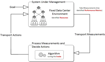
In this section we model the research problem as a closed feedback loop model also called the sense and response system. Given a fixed objective, environment model, and assuming an abstract black-box i.e. a proposed solution algorithm that processes sensed measurements and generates response actions, the feedback model gives us a clear picture of where the resources, knobs and performance metrics identified in problem definition 2.3 fit in and affect the system.
Figure 2.1: Abstract Feedback Model as a Reference Model
2.4.1 Goal
2.4.2 System Under Management
System under management is the complete data center including the switch fabric, the servers and the controller running the algorithm. The data center topology and level of virualization is in accordance with the fixed environment model.
2.4.3 Monitoring
Monitoring captures the accurate system state. The purpose of monitoring the system under management is to get feedback of whether the goals have been met.
Measurement Characteristics: (What, When, Duration, Cost)
What? The measurements variables are resource utilization and tenant requirements. These are the only variables needed to make the decisions of which knobs to tune to get an action.
When? The frequency of measurement is the instance of every new tenant request, i.e. for every request received in the system, resource utilization for the identified resources is measured, and compared with the tenant requirement using the proposed algorithm.Duration? The duration of measurement is from the time instance of the first tenant request received until the time instance of exhaustion of all tenants or the time instance of exhaustion a resource. Cost? The cost of measurement will come in the form of (a) Monitoring agents at the servers, switches and routers (b) Increased storage requirements to store the variables (c) Increased CPU capacity at the servers, switches and routers. The measurements will need to be transferred to a centralized controller running the algorithm.
2.4.4 Processing Measurements and Decide Actions
The purpose of processing the measurements, is analyzing the feedback to determine the action to be taken for a tenant. A tenant can be in three states (a) allocated (b) rejected or (c) re transmitted. The algorithm analyzes the measurement to decide the next state of the tenant.
Processing Characteristics: (Where, Cost)
Chapter 3
Algorithm Design and Key
Questions Formulation
In this chapter we propose three solution algorithms and formulate key design questions that are answered experimentally in Chapter 4.
3.1
Algorithm Design
In this section we present the assumptions made, then we describe the three algorithms pro-posed.
3.1.1 Assumptions
The proposed algorithms rest on the following critical assumptions.
Workload: The algorithms take into account only north bound workload for example video streaming.
Tenant Requirement Distribution:All the tenants in the system are assumed to have randomized requirements in terms of bandwidth and virtual CPUs.
Tenant Period of Datacenter Occupation:A tenant when arrives in the data center, upon allocation of server virtual CPU and uplink bandwidth from server to the core, is assumed to stay there for an infinite period of time.
Number of Distribution and Core Switches:The system is assumed to have two core switches, and two distribution switches per pod. A core can accommodate any number of pods.
Traffic Shapers:The implementation assumes the presence of traffic shapers that limit the uplink traffic sent by tenants in the server to the maximum requirement posed by the tenants at the time of allocation. Though we do not play with traffic shaping as a knob, we suggest rules of thumb for the traffic shapers’ placement in the datacenter.
3.1.2 Greedy Left First Algorithm
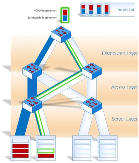
Greedy Left First Algorithm was inspired from the classic bin packing problem, it assumes tenant requirements to be variable sized bins that needs to be packed into fixed size bins that are the servers and paths. The tenant virtual CPU requirements are packed in a greedy left first manner, and similarly the up link path is also consumed in a way that it exhausted the left most up link path firs. As can be visualized in Figure 4.3, the tenants are allocated servers in a greedy left first fashion, and the up link path allocation is also done in a greedy left first manner. The pseudo code for the algorithm uses Algorithms 3, 2, and 1.
Figure 3.1: Generic Fat Tree Topology
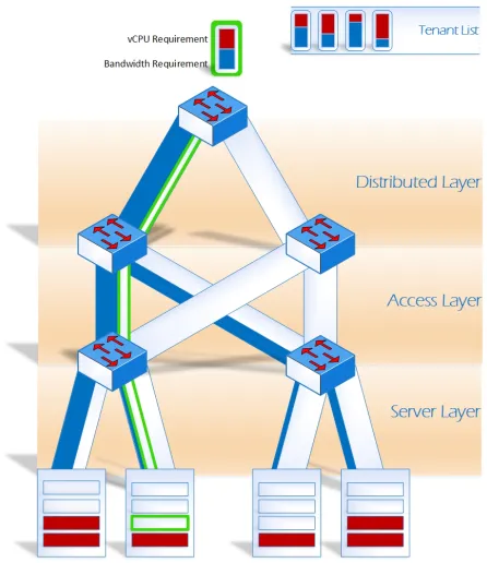
3.1.3 Semi Random Algorithm
Algorithm 1 Allocate Tenant and Decrement Path Resources
1: functionAllocate Tenant and Decrement Path Resources(tenant, path resources)
2: allocate current tenant to the current server
3: decrement tenant virtual CPUs from current server
4: decrement tenant bandwidth from current server uplink, access left uplink, dist uplink(s)
5: go tonext tenant
Algorithm 2 Basic Resource Allocator Algorithm
1: functionBasic Resource Allocator(flag)
2: Get external input parameters
3: Create tenant, server, access, dist switch data structures
4: ifflag == semi-randomthen
5: current server, current access, current dist, current pod←Random Switch Selector Algorithm() 6: else ifflag == greedythen
7: current server, current access, current dist, current pod←server[0], access[0], dist[0], pod[0]
8: whiletenant in tenant queuedo 9: ifflag == semi-randomthen
10: current server, current access, current dist, current pod←Random Switch Selector Algorithm() 11: ifcurrent server has enough virtual CPUsthen
12: ifcurrent server has enough uplink bandwidththen 13: ifcurrent access has enough total uplink bandwidththen 14: ifcurrent access has enough left uplink bandwidththen 15: ifcurrent dist has enough total uplink bandwidththen 16: Allocate Tenant and Decrement Path Resources
17: else if next dist switch has enough uplinkthen 18: ifcurrent access has enough right uplinkthen 19: Allocate Tenant and Decrement Path Resources
20: else
21: Allocate Tenant and Decrement Path Resources using both access uplinks
22: else if both dist switch have enough uplinkthen 23: allocate tenant and update path resources 24: else
25: go tothe next pod
26: else if current access has enough right uplink bandwidththen 27: ifnext dist has enough total uplink bandwidththen 28: Allocate Tenant and Decrement Path Resources
29: else if both dist have enough total uplink bandwidththen 30: Allocate Tenant and Decrement Path Resources
31: elsego tothe next dist pod
32: else if both dist have enough total uplink bandwidththen 33: Allocate Tenant and Decrement Path Resources
34: elsego tothe next dist pod
35: elsecurrent access is the bottleneck,go tonext access switch
36: elsecurrent server bandwidth is the bottleneck,go tonext server
Figure 3.2: Greedy Left First Algorithm
was Greedy Left First algorithm. As can be visualized in Figure 4.4, the tenants are allocated randomly in any servers, and the uplink path allocation is done in a greedy left first manner. The pseudo code for the algorithm uses algorithms 4, 5 and 1.
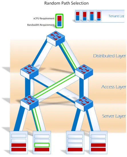
3.1.4 Randomized Algorithm
Randomized algorithm does random virtual machine placement and random path selection. As can be visualized in Figure 4.5, the tenants are allocated randomly in any servers, and the uplink path allocation is also random. The pseudo code for the algorithm uses 6, 7 and 1.
3.2
Key Questions
3.2.1 Datacenter Designer’s Point of View
Given a “Tenant Profile”, What Bandwidth Should I Buy for My Layers?
Algorithm 3 Random Switch Selector Algorithm
1: functionSelect Dist Pod()
2: select random pod
3: ifrequirement fits Dist Podthen returnserver, access, dist, dist pocket
4: elseselect random pod
5: select random pod
6: whilerequirement not fit poddo 7: select random pod
8: ifany resource exhaustedthen 9: Break
returnserver, access, dist, dist pod
10: functionSelect Access()
11: Select Dist Pod()
12: select random access
13: ifrequirement fits Accessthen returnserver, access, dist, dist pocket
14: elseSelect Dist Pod()
15: select random pod
16: whilerequirement not fit Accessdo 17: Select Dist Pod()
18: select random access
19: ifany resource exhaustedthen 20: Break
returnserver, access, dist, dist pod
21: functionSelect Server by Bandwidth()
22: Select Access()
23: select random server
24: ifrequirement fits Server Bandwidththen returnserver, access, dist, dist pocket
25: elseSelect Access()
26: whilerequirement not fit Server Bandwidthdo 27: Select Access()
28: select random access
29: ifany resource exhaustedthen 30: Break
returnserver, access, dist, dist pod
31: functionSelect Server by CPU()
32: Select Server by Bandwidth()
33: ifrequirement fits CPUthen returnserver, access, dist, dist pocket 34: elseSelect Server by Bandwidth()
35: whilerequirement not fit CPUdo 36: Select Server by Bandwidth()
37: ifany resource exhaustedthen 38: Break
returnserver, access, dist, dist pod
39: functionRandom Switch Selector()
40: Select Server by CPU()returnserver, access, dist, dist pod
Algorithm 4 Random Link Selector Algorithm
1: functionRandom Link Selector()
2: select random access link which meets requirement
3: select random dist link which meets requirement
4: whilerequirement not metdo
5: select new random access link, new random dist link
6: ifall access switches exhausted or all dist switches exhaustedthen 7: break
Figure 3.3: Semi Random Algorithm
– How does the error between calculated and experimental server-access bisection bandwidth vary for different server-access configurations
– Should I buy more servers with lesser uplink bandwidth or lesser servers with higher uplink bandwidth. Which configurations yield highest utilization given fixed bisection bandwidth?
Access Layer Characteristics
– How does the error between calculated and experimental access-distributed bisection bandwidth vary for different access-distributed configurations
– Should I buy more access switches with lesser uplink bandwidth and fewer servers per access switch or buy fewer access switches with higher uplink bandwidth and more servers per access switch. Which configurations yield highest utilization given fixed bisection bandwidth?
Distributed Layer Characteristics
Figure 3.4: Randomized Algorithm
bandwidth vary for different distributed-core configurations
– Should I buy more distributed switches with lesser uplink bandwidth and fewer access per distributed switch or buy fewer distributed switches with higher uplink band-width and more access per distributed switch. Which configurations yield highest utilization given fixed bisection bandwidth?
Topology Characteristics
– How does the error between calculated and experimental switch fabric bandwidth vary for different configurations?
– Should I use fewer resources in larger number of pods or larger resources in fewer pods. Which configurations yield highest utilization given fixed switch fabric band-width?
Given a “Tenant Profile”, How Many Servers Should I Buy?
Algorithm 5 Randomized Resource Allocator Algorithm
1: Get external input parameters
2: Create tenant, server, access, dist switch data structures
3: current server, current access, current dist, current pod←Random Switch Selector Algorithm() 4: whiletenant in tenant queuedo
5: current server, current access, current dist, current pod←Random Switch Selector Algorithm() 6: dist link, access link←Random Link Selector()
7: ifcurrent server has enough virtual CPUsthen 8: ifcurrent server has enough bandwidththen 9: ifaccess link is left uplinkthen
10: ifdist link is left OR right OR both uplinksthen 11: Allocate Tenant and Decrement Path Resources
12: else 13: continue
14: else ifaccess link is right uplinkthen
15: ifdist link is left OR right OR both uplinksthen 16: Allocate Tenant and Decrement Path Resources
17: else 18: continue
19: else ifaccess link is both uplinksthen
20: ifdist link is left OR right OR both uplinksthen 21: Allocate Tenant and Decrement Path Resources
22: else 23: continue 24: else 25: continue 26: else 27: continue 28: else 29: continue
– How does the error between calculated and experimental server compute required, vary for different compute per server configurations?
– Should I buy more servers with lesser compute or lesser servers with more compute. Which configurations yield highest utilization given fixed total compute capacity?
3.2.2 Datacenter Administrator’s Point of View
How to Measure Compliance With the Service Level Agreement?
Chapter 4
Implementation and Performance
Evaluation
4.1
Experimental Methodology
4.1.1 Deciding Input Parameters
1. Tenant Bandwidth Requirement: YouTube’s “stream now” for live streaming videos allows customers to choose their own ingestion bit-rate and resolution based on their network conditions. Using the range of bit-rates specified by YouTube for different reso-lutions 4.1 as a basis, the tenants in the system are assumed to be streaming one or more than one videos simultaneously such that the cumulative bit-rate falls in the range 12.5 - 16 Mbps. These values are chosen to comply with the assumed video streaming traffic characteristics.
Table 4.1: Tenant Bandwidth Requirement [18]
Resolution Download Bitrate 1440p@60fps 9 - 18 Mbps
2. Tenant Virtual CPU Requirement: Determining virtual CPU requirement for a media streaming process will depend on the percentage CPU core utilization for that process. If percentage CPU utilization for the process is known, and the number of virtual CPUs tied per core has been decided, we can find out virtual CPUs used by the process in discussion. For example, if a 1080p@30 fps video streaming on an AMD FX 4300 quad core processor is known to utilize 10-25% CPU depending on the type of web browser, i.e. 40 - 100% single core utilization. If each core of the server is theoretically tied to 4 virtual CPUs, then we can assume that 2 - 4 virtual CPUs are used per tenant. This abstraction of virtual CPUs from a CPU core is calculated without any experiments, though a virtual CPU can be mapped to more than one CPU cores at a time, for simplification we assume it be mapped to a single core. This number in reality will be decided by the system designer and we choose to restrict our discussion on this topic, as the basis of our analysis is that the number of virtual CPUs mapped from a CPU core remains fixed throughout. Hence more the virtual CPU count, higher the CPU utilization. So, from the above discussion we assume for bit-rates varying from 720p - 1440p, the number of virtual CPU requirement is varies between 1 - 6 virtual CPUs.
3. Total Number of Tenants: The tenant profile is determined by the tenant bandwidth and virtual CPU requirements, the lower and upper bound of which are fixed. The num-ber of tenants of this profile is varied to analyze the behavior of the system for some experiments, and for others, it is fixed to a random value.
4. Number of Virtual CPUs Per Server: A cost per virtual machine analysis of AMD powered Dell server running Microsoft Hyper-v done by Principled Technologies, com-missioned by Dell [13] envisages the use of Dell M915 blade server with a 16 core AMD processor running Microsoft Windows server as it can host 20 virtual machines for their specific test workload, and deliver equivalent workload outputs with lesser cost per virtual machine when compared to a correspond HP solution. In this analysis we define number of virtual CPUs per server for an abstract server with a 16 core CPU, and ‘x’ virtual CPUs tied to each core, then we can assume each server to have 16∗xvirtual CPUs. This parameter is varied in future analysis.
5. Uplink Bandwidth Per Server: Uplink bandwidth per server depends on the number and capacity of the line cards bought. In this analysis all servers are assumed to have one line card for the uplink traffic towards their corresponding access switch. The capac-ity of the line card is one of the parameters varied to determine the server-access layer bandwidth. No over subscription is assumed.
on the port density and port capacity of the switch. In this analysis all access switches are assumed to have two uplink ports for the uplink traffic towards their corresponding distributed switches. The number of distributed switches are fixed to two for simplicity of implementation, thus the access uplink ports are limited to two. The capacity of the line card is one of the parameters varied to determine the access-distributed layer bandwidth. No oversubscription is assumed.
7. Uplink Bandwidth Per Distribution Switch: The uplink ports for distributed are again fixed to two. As the number of distributed switches is fixed to two per pod, there are no more parameters that can be varied to determine the behavior of the distributed - core layer bandwidth. Therefore logical calculations are used.
8. Uplink Bandwidth Per Core Switch: The uplink bandwidth per core is not considered in this analysis.
Figure 4.1: Abstract topology fixed for the analysis
9. Number of Servers Per Access Switch: The parameter is always greater than or equal to one.
10. Number of Access Per Distribution Switch: The parameter is always greater than or equal to one
11. Number of Distribution Switches Per Pod: This is fixed to two.
4.2
Experiments
4.2.1 Evaluating Proposed Algorithms
1. Why?This section analyzes the behavior of the algorithms proposed in 3.1 to implement the proposed service level agreement. This is done to verify the suitability of the algorithms for answering the key questions posed by the designers and administrators of a data center. 2. How?
(a) Assumed System State:The system gets tenants with a uniform random profile, the number of tenants is varied within a range. The server, access and distributed layer bandwidths are fixed and so is the total number of virtual CPUs and servers. The remaining system state is as described in the assumptions.
(b) Input Parameters Varied: Number of tenants (c) Input Parameters Fixed: All except above
(d) Knobs:We vary server CPU, server bandwidth, access bandwidth and distributed bandwidth in separate experiments such that each of them become bottlenecks. The idea is to observe the behavior of the compute and SF utilization when in bottleneck. (e) Metrics: Mean Server virtual CPU Utilization, Mean Server, Mean Access and Mean Distributed Layer Bandwidth Utilization are compared to observe the overall behavior of the algorithms.
No Bottleneck
1. Assumed System State: The system is in no bottleneck state which means that all the layers’ bandwidth is sufficient to accommodate all tenants, and similarly server compute is also sufficient enough to accommodate maximum tenants
2. Specific Knob: All the resources are over-provisioned in the system, and the number of incoming tenants are varied.
4. Inference: Random and semi-random algorithms give higher resource utilization when there is no bottleneck as compared to the greedy algorithm of the order of magnitude 2%. Since the difference may easily encompass the confidence interval range, it can be ignored.
Figure 4.2: Percentage resource utilization when no bottleneck in the system.
Server CPU as a Bottleneck
1. Assumed System State: The system is in a server CPU bottleneck state which means that all the layers’ bandwidth are sufficient to accommodate all tenants, but server com-pute is not enough to accommodate the given tenants
2. Specific Knob: Server CPU is provisioned to be a bottleneck for the given tenant profile and number. All the remaining resources are over-provisioned in the system to never become a bottleneck before server CPU, as the number of incoming tenants are varied. 3. Observation: The mean server CPU utilization for the greedy algorithm is lesser than
that for the semi-random and random algorithm. The difference is in the order of 3-4%, However the SF utilization only sees a jump of 1.5 - 2% when moving from greedy to semi-random and random algorithms. The difference was expected due to servers not being shared among tenants.
Figure 4.3: Percentage resource utilization when server CPU is bottleneck
Server Uplink Bandwidth as a Bottleneck
1. Assumed System State: The system is in server uplink bandwidth bottleneck state which means that all the layers’ bandwidth is sufficient to accommodate all tenants ex-cept the server-access layer bandwidth which is less than the tenant requirement. Server compute is sufficient enough to accommodate maximum given tenants
2. Specific Knob: Server layer bandwidth is provisioned to be a bottleneck for the given tenant profile and number. All the remaining resources are over-provisioned in the system to never become a bottlneck before server bandwidth, as the number of incoming tenants are varied.
3. Observation: The mean server CPU utilization for the greedy algorithm is similar that for the semi-random and random algorithm. The difference is in the order of 0-0.32%, However the SF utilization only sees a jump of ˜0.2% when moving from greedy to semi-random and semi-random algorithms. The lesser difference among algorithms was expected due to server bandwidth not being shared by two or more servers.
4. Inference: Server bandwidth bottleneck state does not affect the compute and SF uti-lizations obtained from all the proposed algorithms.
Access Uplink Bandwidth as a Bottleneck
Figure 4.4: Percentage resource utilization when server bandwidth is bottleneck
the access-dist layer bandwidth which is less than the tenant requirement. Server compute is sufficient enough to accommodate maximum given tenants
2. Specific Knob: Access uplink bandwidth is provisioned to be a bottleneck for the given tenant profile and number. All the remaining resources are over-provisioned in the system to never become a bottleneck before access uplink bandwidth, as the number of incoming tenants are varied.
3. Observation: The mean access bandwidth utilization for the three proposed algorithms doesn’t vary when access bandwidth is a bottleneck. This near zero difference is due to access layer is shared among tenants in a similar fashion, with server not being a bottleneck this is an expected result.
4. Inference: Access bandwidth bottleneck state does not affect the compute and SF uti-lization obtained from all the proposed algorithms.
Distribution Uplink Bandwidth as a Bottleneck
1. Assumed System State: The system is in distributed uplink bandwidth bottleneck state which means that all the layers’ bandwidth is sufficient to accommodate all tenants except the distributed-core layer bandwidth which is less than the tenant requirement. Server compute is sufficient enough to accommodate maximum given tenants
Figure 4.5: Percentage resource utilization when access uplink bandwidth is bottleneck
system to never become a bottleneck before distributed uplink bandwidth, as the number of incoming tenants are varied.
3. Observation: The mean distributed bandwidth utilization for the three proposed algo-rithms doesn’t vary when distributed bandwidth is a bottleneck. This near zero difference is due to distributed layer is shared among tenants in a similar fashion, with server not being a bottleneck this is an expected result.
4. Inference: Distributed bandwidth bottleneck state does not affect the compute and SF utilization obtained from all the proposed algorithms.
Tenants Served
1. Assumed System State: The system is put into all bottleneck states one by one as above, and maximum number of tenants served in each case is observed.
2. Specific knob: Tenants served are calculated for all of the bottleneck states.
3. Observation: Tenants given a tenant profile served were the least when server CPU Utilization is a bottleneck, 21 more tenants were served when server bandwidth was a bottleneck. With access and distributed layer as bottlenecks, the tenants served increase by approximately 17
4. Inference: The number of tenants served increases as the bottleneck goes up the layers.
Figure 4.7: Number of tenants served when the given resources are bottleneck or no system bottleneck
Summary
4.2.2 What Bandwidth Should I Buy for My Layers?
This section develops an approach to decide the bandwidth that a data center designer should buy for the switch fabric. Two key parameters affect this decision
-1. Minimum Bandwidth Required to Allocate Resources for Given Tenants: This can be logically estimated if the tenant profile and maximum number of tenants are known.
2. The Topology to Distribute Estimated Bandwidth: Once the overall switch fabric bandwidth is known, a finer granularity of the bandwidth per port per switch, and per NIC per server, number of switches and servers, needs to fixed. This is done by fixing a minimal topology for the data center.
It is assumed that the designer knows the total compute required to serve a fixed number of tenants. Before describing the experiments, the assumptions and overall experimental method-ology is discussed. The assumptions and methodmethod-ology specific to the experiments are discussed in corresponding subsections.
1. Assumptions:
The tenant profile remains fixed
The total compute required required by all tenants is known to the designer, and it is fixed to a value such that server CPU never becomes a bottleneck.
The tenants are assumed to be never leave the system once they are allocated the resources.
No oversubscription is assumed.
2. Experimental Methodology:
Estimate Layer-Level Local Bandwidth: Per-layer minimum bisection band-width is estimated, along with correspond per port/NIC bandband-width for switches/servers.
Criterion for Estimation:
– Logical vs. Experimental Estimation: Variance of error between logically estimated minimum bandwidth and experimental minimum bandwidth with dif-ferent switch fabric profiles
– Scalability w.r.t Tenants: Variance of the bottleneck bandwidth utilization with number of tenants
Estimate Overall Switch Fabric Bandwidth
Server Layer Characteristics
1. Experiment 1
Goal: Estimate variation in the error between calculated and experimental server-access bisection bandwidth for different server-server-access configurations
Assumptions:
(a) Server CPU, access-distributed bisection bandwidth and distributed-core bisec-tion bandwidth are over-provisioned such that none ever become bottlenecks. This helps assessing the behavior of server-access bisection bandwidth without any internal system influence.
(b) Number of access switches per pod and distributed switches per pod are both fixed to two. The number doesn’t affect the analysis as long as the access-distributed-core bandwidth is over-provisioned.
(c) Number of tenants are fixed to 1400. This is a randomly chosen number. (d) Number of pods are fixed to one, which keeps the topology minimal, keeping the
analysis simpler.
Experimental Methodology:
(a) Total number of servers and virtual CPUs per server are varied such that total virtual CPUs remain constant, number of servers are incremented and virtual CPUs per server are decremented to keep the total compute constant.
(b) For each of server combination, a minimum server-access bisection bandwidth and corresponding uplink server bandwidth per server is calculated using the average tenant requirement
(c) For each of server combination, a minimum server-access bisection bandwidth and corresponding uplink server bandwidth per server are experimentally calcu-lated
(d) Percentage error is calculated between the calculated and experimental values, and the trend of the error is observed.
Observations:
(a) As can be seen in Fig. 4.8 error between the calculated and experimental server-access bisection bandwidth increases positively as with the increase in the num-ber of servers with corresponding smaller bandwidths.

![Table 4.1:Tenant Bandwidth Requirement [18]](https://thumb-us.123doks.com/thumbv2/123dok_us/1539063.1188772/41.612.223.410.514.630/table-tenant-bandwidth-requirement.webp)