ABSTRACT
ALANEZY, KHALID ALI. Optimal Control of Moving Interface and Phase-Field Separations. (Under the direction of Kazufumi Ito.)
In this thesis we consider two moving interface problems of practical interests. The first one is the sharp interface model of solidification by the classical two-phase Stefan problem, and the second one is the phase-field model by the coupled Cahn-Hilliard Navier-Stokes system. The main objective of this thesis is to formulate the optimal control problem for the motion of the change of phase and phase separation of the binary fluid mixture by the boundary control. The Lagrange calculus is used in the analysis of the two highly non-linear and non-smooth control problems. Phase changing and phase separation are considerably involved with a lot of applications in industry.
For the case of two-phase Stefan problem, our objective is to control the motion of the solidification interface by formulating a tracking type optimal control problem. The control we use is the heat flux at a portion of the boundary, so that we achieve a desired solidification motion by the boundary control.
For the Cahn-Hilliard Navier-Stokes system, our main goal is to control the separation of the two fluids by the boundary control of the fluid velocity field. The Navier-Stokes equations are coupled to the Cahn-Hilliard system in the following way. The velocity field introduces the transport term of the concentrations in the Cahn-Hilliard equations, the fluid structure interaction force is added into the incompressible Navier-Stokes equations as an interaction force, and our control enters as a Dirichlet boundary condition for the velocity field.
Optimal Control of Moving Interface and Phase-Field Separations
by
Khalid Ali Alanezy
A dissertation submitted to the Graduate Faculty of North Carolina State University
in partial fulfillment of the requirements for the Degree of
Doctor of Philosophy
Applied Mathematics
Raleigh, North Carolina 2017
APPROVED BY:
Ernest Stitzinger Lorena Bociu
Ralph Smith Kazufumi Ito
DEDICATION
BIOGRAPHY
The author was born in 1986 in Saudi Arabia, and raised with his three brothers and five sisters. He is married and has two sons and one daughter.
The author attended King Fahd University of Petroleum and Minerals (KFUPM) where he received his Bachelor’s degree in Mathematics in 2009 and his Master’s in Applied Mathematics in 2012. On his Master’s thesis, he was supervised by Dr. M. Tahir Mustafa. The title of his Master’s thesis was ”Group of Classification and Similarity Solutions of Klein Gordon Equations on a Sphere”.
ACKNOWLEDGEMENTS
First and foremost, I would like to thank my advisor Professor Kazufumi Ito for his guidance, patience and valuable advices. His help and support were essential in the successful completion of this thesis.
I would also like to thank the rest of my thesis committee members: Dr. Ernest Stitzinger, Dr. Ralph Smith and Dr. Lorena Bociu for their invaluable inputs and advices.
I am also grateful to my parents who have loved and enabled me throughout my life and enlighten me to realize the value of an education. They have taught me hard work and patience. My sincere thanks go to my wife for her continuous support, care and encouragement throughout the years.
TABLE OF CONTENTS
LIST OF FIGURES . . . vii
Chapter 1 Introduction . . . 1
Chapter 2 The Classical Two-Phase Stefan Problem. . . 8
2.1 Enthalpy Formulation of the Two-Phase Stefan Problem . . . 8
2.2 Strong Form of the Two-Phase Stefan Problem . . . 10
2.3 Weak Solution of Enthalpy Formulation . . . 12
2.3.1 An Apriori Bound of the Finite Difference Solution . . . 14
2.4 Convergence of Weak Solutions . . . 16
2.4.1 Aubin’s Lemma . . . 16
2.4.2 Passing the Limit asλ→0 Using Aubin’s Lemma . . . 17
2.5 Lipschitz Continuity of Solution E with Respect to Controlg . . . 20
Chapter 3 Optimal Control Problem for the Motion of the Interface of Stefan Problem . . . 22
3.1 Existence of Optimal Control . . . 23
3.2 Lagrangian Functional and Adjoint Equation . . . 24
3.2.1 Existence of the Adjoint Statep . . . 24
3.2.2 An Apriori Bound for Solution of Adjoint Equation . . . 25
3.3 Necessary Optimality Condition . . . 26
3.4 Numerical Methods for Enthalpy Formulation of the Controlled Tow-Phase Ste-fan Problem . . . 26
3.4.1 Numerical Test Examples . . . 30
Chapter 4 Cahn-Hilliard Navier-Stokes System . . . 37
4.1 Weak Formulation of Cahn-Hilliard System . . . 40
4.2 Incompressible Flow by Navier-Stokes Equations . . . 41
4.2.1 Navier Boundary Conditions and Slip Functions . . . 43
4.2.2 Weak Formulation of Navier-Stokes Equations . . . 44
4.3 Sharpened and Obstacle Ginzburg-Landau Potential . . . 46
4.4 Constructing a Weak Solution of Cahn-Hilliard Navier-Stokes System . . . 49
4.4.1 An Apriori Estimate for the Weak Solution . . . 50
4.4.2 Applying Aubin’s Lemma to Pass the Limit asn→ ∞ . . . 54
4.5 Lipschitz Continuity of Solution with Respect to Velocity Boundary Control . . . 58
4.6 Semi-Group Analysis for Cahn-Hilliard Equations . . . 60
4.6.1 Nonlinear Semi-Group Theory for Cahn-Hilliard Equations . . . 61
4.6.2 Linear Semi-Group Theory . . . 62
4.6.3 Lifting Regularity of c(t) . . . 62
4.7 L2(0, T ×Ω) Lagrange Multiplier for Obstacle Potential . . . 65
5.1 Existence of optimal controls . . . 69
5.1.1 Weak Continuity of Equality Constraint . . . 70
5.2 Necessary Optimality Using Lagrange Calculus . . . 70
5.2.1 An Apriori Bound for Galerkin Solutions of the Adjoint System . . . 72
5.3 Numerical Methods for Cahn-Hilliard Navier-Stokes System . . . 75
5.3.1 Numerics and Discretization of Navier-Stokes System . . . 78
Chapter 6 Summary and Conclusion . . . 83
Bibliography . . . 85
APPENDICES . . . 91
Appendix A Optimization Theory . . . 92
A.1 Existence of Minimizers . . . 93
A.2 Lagrange Multipliers Theory and Complementarity Condition . . . 94
Appendix B Lagrange Calculus . . . 96
B.1 Necessary Optimality Condition . . . 96
B.1.1 Stefan Problem Case . . . 98
B.1.2 Cahn-Hilliard Navier-Stokes Case . . . 98
Appendix C Incompressible Navier-Stokes Equations . . . 100
C.1 Leray Projection of f on H0 and H . . . 100
C.2 Hodge-Decomposition . . . 101
Appendix D Numerical Methods . . . 103
D.1 Semi-smooth Newton’s Method . . . 103
D.2 Sequential Programing Method . . . 106
LIST OF FIGURES
Figure 1.1 Freeze cast process . . . 2
Figure 1.2 Splitting of solid region (blue) by boundary flux . . . 4
Figure 1.3 Submerged gas injection into metallurgical refining process . . . 5
Figure 1.4 Separation with rotating velocity field . . . 6
Figure 2.1 The enthalpy set-valued graph γ(T) . . . 10
Figure 2.2 The Inverse of Enthalpy Graph β(E) . . . 11
Figure 3.1 The value of the temperature is at the center of the cell . . . 28
Figure 3.2 The control boundary Γc. . . 30
Figure 3.3 Splitting of solid region (blue) by boundary flux . . . 31
Figure 3.4 The full horizon target state . . . 32
Figure 3.5 Half horizon result . . . 33
Figure 3.6 The resultant optimal control on the half horizon . . . 34
Figure 4.1 The graph of the transition layer . . . 38
Figure 4.2 Ginzburg-Landau potential: standard-sharp-obstacle . . . 47
Figure 5.1 The velocity is located at the nodal points . . . 78
Figure 5.2 Divergence term divv located at i, j pressure node . . . 79
Chapter 1
Introduction
In this thesis we will study two important moving interface problems of practical interests. In particular, we will focus on control of the interface motion. The first problem is the sharp interface model of solidification by the classical two-phase Stefan problem [10, 41, 42, 15, 44]. The second one is the phase-field model for the separation of two fluids by the coupled Cahn-Hilliard Navier-Stokes system [2, 4, 18, 31, 12]. Those two problems are related to each other, since the limit of the phase-field model is given by the sharp interface model.
Our objective is to introduce a mathematical formulation of the two models based on vari-ational approach using the corresponding energy functional. Most importantly, our analysis is developed for each model with boundary control. Then, we formulate the optimal control problem for each case and derive the necessary optimality condition. Based on the optimality condition, we develop numerical algorithms to find the optimal control. The analysis of those two problems helps us to promote the study of different moving interface problems.
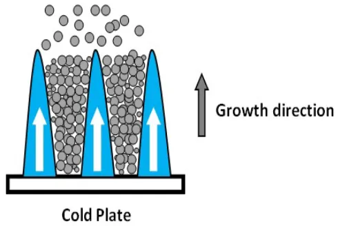
The two-phase Stefan model is widely used in the field of industry. For example, it is used in the freeze-cast method which is utilized to make porous ceramics [57]. In industry fields, they first prepare ceramic slurry and then freeze it on a cold surface to produce the desired ceramic. Porous ceramics have low thermal conductivity and therefore they are utilized in filters, thermal insulation and energy devices. The process of making porous ceramics begins by pouring the slurry into a mould which undergoes isotropic cooling to induce solidification, as shown in Figure (1.1). In order to have certain mechanical properties of pore networks of freeze
Figure 1.1 Freeze cast process
cast ceramics, we focus mainly on porosity and pore size. Pore size decreases with increasing freezing front velocity, i.e. the speed at which the solid-liquid interface advances. The interface velocity increases with decreasing freezing surface temperature. To be able to use freeze cast products commercially, we need to have a specially designed casting setup in which we can determine processing conditions that gives a set of pore network characterizations a priori. Since pore size is determined by velocity of freezing front, a pore size model must include an effective method to predict the velocity of freezing interface which can be achieved using the two-phase Stefan model. The importance of determining solidification front velocity arises in different industrial processes such as metal casting and crystal growth.
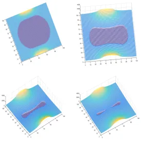
solid region (dark blue), surrounded by a liquid region (light blue) and a boundary heat flux at a portion of the boundary Γc. After some time, we see the evolution of the interface region, which
leads to shrinking of the solid region till the solid region splits into two pieces. Our control can be accomplished by tracking a desired interface motion and constructing the cost functional in which we regulate the difference between the graph of the physical interface and the desired interface [10, 41, 42]. The control uses the flux at a portion of the exterior boundary to design the motion of the interface.
In the classical approach based on the two phase Stefan problem, we must determine the motion of the interface Γt along with the solutions to heat equations on each phase via the
interface condition. But we use the equivalent formulation of the Stefan problem based on the enthalpy formulation. The enthalpy is the total thermal energy and is a monotone piecewise linear function of temperature. The enthalpy satisfies the nonlinear (non-smooth but monotone) heat equation with boundary heat flux control. The control enters into the equation as the boundary heat flux control on a portion of the boundary. During the process of phase changing, a latent heat is either released out or absorbed by the system at the interface. The latent heat exchange causes a discontinuity (or a jump) on the enthalpy at a critical solidification temperature, and yields to a thickness of the interface layer [8, 9]. One can derive the weak form of the enthalpy equation in which the boundary control appears naturally as the boundary integral in the weak form. Then, we study the existence and regularity properties of weak solution for the enthalpy formulation, e.g. see [46, 64, 20]. The temperature is then determined as a function of the enthalpy. The advantage of the enthalpy formulation is that it is more effective to develop the mathematical formulation with boundary control and also develop numerical analysis for the solutions of the problem.
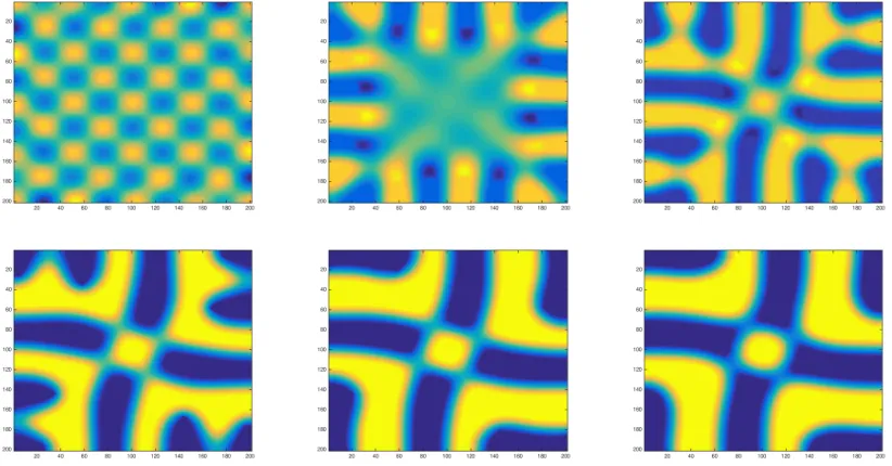
The second problem is the physical phenomena of phase separation of a binary fluid mixture. We use the Cahn-Hilliard equation as a mathematical model for the phase separation. The two components could refer, for example, to water and oil. When an alloy, that is a mixture of two metallic components, is heated, and then cooled quickly to a lower temperature, a phase separation can occur suddenly. This separation of the metal alloy into two components, by lowering the temperature of the mixture, is known as spinodal decomposition [14].
Figure 1.2 Splitting of solid region (blue) by boundary flux
nickel appears. After some time, these formation of pure phases coarsen into larger ones. It is very important to understand the dynamic of the formation of this coarsen regions which leads to the process of separating the two components. The separation process of the two components occurs along with pattern formation and evolution.
Figure 1.3 Submerged gas injection into metallurgical refining process
have a quantitative information of gas-liquid flow. Thus, the diffuse interface method is used to predict the behavior of argon gas injection into the molten aluminum. The Computational fluid dynamics modeling for injection process is formulated by using the coupled Cahn-Hilliard Navier-Stokes system. The system describes the flow induced by the argon gas and models the dynamic evolution of the interface layer between gas plume and liquid metal. In the diffuse interface methods, the evolution of the interfacial layer is governed by a phase-field variable c
that obeys the convective-diffusion Cahn-Hilliard equation.
Figure 1.4 Separation with rotating velocity field
control the separation indirectly based on Cahn-Hiiliard Navier-Stokes model. Because of the fluid-structure interaction force, we can control the fluid by the boundary control of the fluid [38, 39]. Examples of control actions include sliding, rotation, injection and sucking. Understanding the dynamic of the separation has been the subject of much research in the 20th century [27].
The plan of this thesis is as follows. In Chapter 2 we focus on the solidification problem. First, we develop the variational formulation of enthalpy equation with boundary control, based on the thermal energy for the two phase Stefan problem and the corresponding weak form of equations [59, 19, 24]. Second, we show the existence of weak solutions with the help of Aubin’s lemma. Then, we prove the Lipschitz continuity of solutions with respect to boundary control and initial conditions.
In Chapter 3 we formulate the optimal boundary control problem of tracking the desired motion for the solidification interface and show the existence of optimal control. Next, we derive the necessary optimality using the Lagrange calculus. We also develop numerical discretization method with control to construct the optimal boundary control based on the sequential pro-graming for the necessary optimality condition [47]. Lastly, we present some numerical test examples for achieving a desired solidification.
energy formulation and the corresponding weak form of equations [51, 36]. Second, we show the existence of weak solutions. We also prove the Lipschitz continuity of solutions with respect to velocity control and initial conditions using the Galerkin approach and Aubin’s lemma for the compactness of Galerkin solutions. We use semi-group theory to lift regularity of concentration
c. Also, we consider the sharpened Ginzburg-Landau potential as in [36, 37] as a specific model for our analysis and numerics. As done in [36], we obtain the chemical potential for the obstacle potential, i.e. the concentrationc is constrained to|c| ≤1, for the phase separation in terms of theL2-multiplier and the complementary condition.
In Chapter 5 we formulate the optimal boundary control problem of tracking a desired state. We derive the necessary optimality using Lagrange calculus. We also develop numerical methods with control to construct the optimal boundary control.
For the optimal control problems in both models, it is not straight forward to apply directly the standard Lagrange multiplier theory [47], since we need to introduce function spaces which are different from Gelfand-triple formulation. Thus, we use the so-called Lagrange calculus ap-proach, as in [47], to derive the necessary optimality. The details of Lagrange calculus approach are described in Appendix B.
Chapter 2
The Classical Two-Phase Stefan
Problem
In this chapter we focus on the classical two-phase Stefan problem. First, we introduce the enthalpy formulation of the problem. Then, we derive the differential form of the two-phase Stefan model based on the enthalpy formulation. Next, we show the existence of weak solutions of the enthalpy formulation with the help of Aubin’s lemma. We also prove Lipschitz continuity of solutions with respect to control and initial conditions.
Stefan problem is a moving interface model that describes change of phase, as in, for ex-ample, solidification or melting of ice. The change of phase occurs in a mushy zone, called the interface, where the liquid and solid phases are present simultaneously. The model has important applications in natural sciences and industrial processes [61], as described in the introduction.
2.1
Enthalpy Formulation of the Two-Phase Stefan Problem
In the classical temperature formulation of the two-phase Stefan problem, the location of the moving interface has to be determines as part of the solution and cannot be identified in advanced. Therefore, solutions based on this formulation become difficult to analyze, especially in multidimensional problems. Alternatively, there have been many formulations developed to analyze free boundary problems. The enthalpy method is widely used in solving the two-phase Stefan problem as it reformulates the heat conduction equation to involve the internal energy represented by enthalpy without the need to regard the motion of the interface as an explicit boundary condition.
Enthalpy, as a function of temperature, is a measurement of energy in a thermodynamic system. It is the thermodynamic quantity equivalent to the total heat content of a system, i.e. the sum of the specific heat and the latent heat. Recall that the standard single-phase heat conduction equation with flux controlg is given by
Et= (ρcθ)t=κ∆θ, κ
∂θ
∂ν =g, (2.1)
where θ(x, t) is the temperature at any point x ∈ Ω and time t > 0, E is the enthalpy given by E=ρcθ. Here ρ(x)>0 is the mass density,c=c(θ) is the specific heat, as a function of θ, and gis the flux control at portion of the boundary Γc. The specific heat can be defined as the
amount of heat per unit mass required to raise the temperature by one degree Celsius.
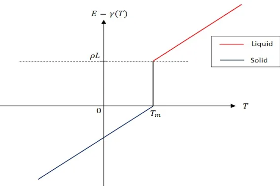
Now, we introduce the enthalpy law for dual-phase, i.e. solid and liquid. The difference between the single phase and dual phases, that the enthalpy has a jump at a critical solidification temperature Tm with jump sizeρL, due to latent heat exchange. The latent heatL is defined
as the energy released or absorbed by a thermodynamic system. This jump condition is often called Stefan condition. In Figure (2.1), one can see the enthalpy graph [20, 8, 61], defined as,
γ(T) =
ρc`(T −Tm) +ρL, T ≥Tm,
[0, ρL], T =Tm,
ρcs(T−Tm), T ≤Tm.
(2.2)
where T = θ is the temperature, ρ is the mass density of solid and liquid, cs, cl are specific
heat of solid and liquid, respectively, and Lis the latent heat.
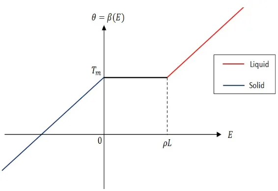
On the other hand, the inverse of the set-valued graphγ, defined by (2.2) isθ=β(E), a function of the enthalpy as in Figure (2.2). That is,
β(E) =
Tm+
1
ρc`
(E−ρL), E ≥ρL,
Tm, 0≤E ≤ρL,
Tm+
1
ρcs
E, E≤0.
(2.3)
Observe that θ = β(E) is a continuous nondecreasing Lipschitz function in E. Conversely, γ
Figure 2.1 The enthalpy set-valued graphγ(T)
Thus, the equation of enthalpyE can be written as
Et=∇ ·(κ∇β(E)), κ
∂
∂νβ(E) =g. (2.4)
So, if the enthalpy E is given, then the temperature is defined by θ = β(E), and hence the interface is defined by {θ=Tm}.
2.2
Strong Form of the Two-Phase Stefan Problem
In this section we discuss the strong differential form of the two-phase Stefan problem. We introduce the moving interface problem based on our enthalpy formulation. First, we define the interface set Γt as
Γt={x∈Ω :θ(t, x) =Tm}
where Γt is assumed to be a surface representing the interface between the solid region Ω−t
whereθ < Tm, and the liquid region Ω+t whereθ > Tm, with Ω−t ∩Ω+t = Γt, and Γt is the free
common boundary (interface) in between the two regions. The solidification temperature at the interface is assumed to be constant and equalsTm.
The standard vector form of the single-phase heat conduction equation is
ρ c∂T
Figure 2.2 The Inverse of Enthalpy Graphβ(E)
whereT is the temperature,ρis the material density,cis the specific heat, andκis the thermal conductivity of the material. Thus, we have the separate heat conduction for each phase, i.e. liquid and solid phases, as
ρcs
∂Ts
∂t =κs∆Ts, for x∈Ω
−
t
ρc`
∂T`
∂t =κ`∆T`, for x∈Ω
+
t.
The boundary flux control for (2.5) is given by
κ ∂
∂νT =g, (2.6)
at a portion Γc of the exterior boundary ∂Ω, which is the control portion, and otherwise the
flux is zero at∂Ω\Γc.
We are interested in tracking the motion of the interfaceX(t) = {x∈Ω : θ(t, x) =Tm} on Γt
in the normal direction, i.e.
d
where V(t, X(t)) is the velocity of the interface motion. By the distribution theory, the latent heat of the systemL, is related to the difference of flux as
Z
Γt
(ρLd
dtX(t))φ ds=
Z
Γt
[κ∂T ∂ν]φ ds
for all smooth functionsφ. Thus, we have
ρL V(t, X(t)) = [κ∂T
∂ν]Γt =κ`
∂T`
∂ν −κs ∂Ts
∂ν (2.7)
whereκ`, κs are conductivity of liquid and solid, respectively. Thus, we have a jump condition,
often called Stefan condition, on Γtwhich determines the evolution of the interface motion with
velocityV(t, x(t)).
In summary, the governing equations for the differential form of Stefan problem are given by
ρscs
∂Ts
∂t =κs∆Ts, for x∈Ω
−
t , Ts=Tm, on Γt
ρ`c`
∂T`
∂t =κ`∆T`, for x∈Ω
+
t , T`=Tm, on Γt
ρL V(t, X(t)) = [κ∂T
∂ν], on Γt.
(2.8)
By the last equation, we compute the flux differences and determine the evolution of the inter-face. In the system (2.8), the unknown pair is (T,Γt), where T is the temperature field and Γt
is the interface location. Thus, if the interface Γt is given, we can determine the temperature
at each phase, and control the motion of the free boundary.
2.3
Weak Solution of Enthalpy Formulation
In this section we show the existence of weak solutions to the enthalpy formulation with bound-ary control. First, we introduce the weak form of enthalpy equation. Then, we establish an apriori bound for enthalpy solutions.
For a fixed domain Ω with Γc ⊆ ∂Ω, the enthalpy formulation can be written using Green’s
formulas as
Z
Ω
Etφ dx=
Z
Ω
(κ∆θ)φ dx= Z
Γc
g φ ds−
Z
Ω
for all test functionsφ∈H1(Ω), where we usedκ ∂
∂νθ=g. The advantage of writing the weak
form is that the controlgappears explicitly in the weak form (2.9). Equation (2.9) is equivalent to
(κ∆θ, φ) =−κ(∇θ,∇φ)Ω+κ(∂θ
∂ν, φ)Γc =−(κ∇θ,∇φ)Ω+ (g, φ)Γc. (2.10)
We construct the weak solution of (2.9) by considering the difference scheme in time for (2.4)
En−En−1
λ =κ∆β(E
n), κ ∂
∂νβ(E
n) =gn, (2.11)
whereλ >0 is the time step size. Letθn=β(En), then (2.11) can be written as
En−En−1=τ∆θn, κ ∂ ∂νθ
n=gn, (2.12)
where τ = κλ. Now, let j : R → R be a strictly convex functional, and its sub-differential
∂j =γ(·) is a maximal monotone graph. The functional j can be written as
j(θ) =
1 2ρcsθ
2, θ≤0,
1 2ρc`θ
2+ρLθ, θ≥0,
(2.13)
whereθ=T −Tm. Then, equation (2.12) can be written as
τ∆θn+En−1 ∈∂j(θn), κ∂θ
n
∂ν =g
n, (2.14)
since ∂j = γ is a set-valued graph. We define the solution of (2.12) by minimizing the cost functional
1 2
Z
Ω
(τ|∇θ|2+j(θ)−En−1(x)θ)−λ(gn, θ)Γc dx, ∀θ∈H
1(Ω). (2.15) Since the minimizing formula (2.15) is quadratic, then it is coercive and strictly convex in θ. Thus the existence of a unique solution is guaranteed. Indeed, given En−1 and gn, then the minimizer θ ∈ H1(Ω) of (2.15), is the unique solution of (2.14), given that En ∈ L2(Ω) and
2.3.1 An Apriori Bound of the Finite Difference Solution
Now, we establish an apriori bound for the difference scheme solutions in order to be able to pass the limit asλ→0. First, let
Φ(E) = Z E
0
β(z)dz =TmE+
1 2ρcs
|E|2, E ≤0,
0, 0≤E ≤ρL,
1 2ρc`
|E−ρL|2, E ≥ρL.
(2.16)
Then, Φ is convex. Recall the basic inequality for differentiable convex functions
f(x)≥f(ˆx) +∇f(x)T(x−xˆ), ∀xˆ∈ domf. (2.17) Now, we show theL2estimate for∇θnandEn, i.e.∇θn∈L2(0, T;L2(Ω)) andEn∈L∞(0, T;L2(Ω)). First, recall equation (2.12)
En−En−1 =τ∆θn,
where
∇θn=β0(En)∇En. (2.18)
sinceθn=β(En). Also, from equation (2.17) we have
Φ(En−1)−Φ(En)≥(Φ0(En), En−1−En) which implies that
Φ(En−1)−Φ(En)≥(β(En), En−1−En). (2.19) Substituting θn=β(En) in (2.19), we get
Φ(En−1)−Φ(En)≥(θn, En−1−En).
So, we get
(En−En−1, θn)≤Φ(En)−Φ(En−1). (2.20) Now, by Green’s identities we have
Then, it follows from (2.11) that Z
Ω
Φ(En)dx−
Z
Ω
Φ(En−1)dx+τ|∇θn|2≤λ(gn, θn)Γc, (2.21)
Then, summing (2.21) in time, we obtain Z
Ω
Φ(En)dx+
n
X
k=1
κλ|∇θn|2 ≤
Z
Ω
Φ(E0)dx+
n
X
k=1
λ|gn|2L2(Γ). (2.22)
whereθn=β(En), andβ(En) is Lipschitz. Note that
(θn, gn)≤ |θn|H1(Ω)|gn|H−1/2(Γ
c). (2.23)
Estimating |∇θn| in (2.22) is not enough for the full H1-norm, since the full norm of θn in
H1(Ω) is given by
|θn(t)|2
H1(Ω)= (θn, θn) + (∇θn,∇θn).
Now, we have the L2 bound forθn is given by
|θn(t)|
L2(Ω)≤C0|En|2 ≤C1Φ(En) +C2. (2.24)
Thus, there exists some constantC >1 such that Z
Ω
Φ(En)dx+ 1 2
n
X
k=1
κλ|β0(En)∇En|2 ≤
Z
Ω
Φ(E0)dx+C
n
X
k=1
λ|gn|2L2(Γ). (2.25)
Also, we have theL1 bound ofEn as follows. In fact, from (2.11), we have
(En−En−1, ρε(θn) =
Z
Ω
∆θnρε(θn)dx=
Z
Γ
∂θn ∂ν ρε(θ
n)ds−
Z
Ω
|∇θn|2 ρ0
ε(θn)dx
So,
Z
Ω
|En| −
Z
Ω
|En−1| ≤λ
Z
Γc
|gn|ds (2.26)
Therefore, we get
Z
Ω
|En|dx−
Z
Ω
|E0|dx≤λ
n
X
k=0 Z
Γc
which implies that
Z
Ω
|En|dx≤M, (2.27)
and then, we obtain the following estimate Z
Ω
θndx= Z
Ω
β(En)dx≤L
Z
Ω
|En|dx≤LM. (2.28)
where L is the Lipschitz constant of β(En). This estimate completes the full norm in H1 and it is enough for us to be able to pass the limit asλ→0.
2.4
Convergence of Weak Solutions
In this section we show the existence of weak solution of enthalpy formulation (2.9) by passing the limit as λ → 0 using Aubin’s lemma. First, we discuss the statement of Aubin’s lemma. Then, we apply Aubin’s lemma to pass the limit in (2.11) and prove the existence of weak solutions.
2.4.1 Aubin’s Lemma
Aubin’s lemma is an important result in Sobolev spaces theory. The theorem gives a criterion for the compact embedding inL2(0, T;X). The Lemma is useful in the study of nonlinear evolution equations. In particular, it helps us to prove the existence of approximate solutions constructed using Galerkin method. The statement of Aubin’s lemma is given as follows.
Aubin’s Lemma:
Let X0, X and X1 be Banach spaces with X0 ⊆X ⊆X1 and X0 is compactly embedded in the pivoting spaceX andX is continuously embedded in X1. Assume thatX0 andX1 are reflexive. Then
W :={u∈L2(0, T;X0) :ut∈L2(0, T;X1)} is compactly embedded into L2(0, T;X).
2.4.2 Passing the Limit as λ →0 Using Aubin’s Lemma Recall equation (2.4) which can be written as
Et=κ∆θ, κ
∂θ
∂ν =g, (2.29)
and recall from last section that
θn∈L2 0, T;H1(Ω)
, and ∇θn∈L2 0, T;L2(Ω)
.
In order to be able to use Aubin’s lemma, we need to show that
En∈L2 0, T;H1(Ω), and dE
n
dt ∈L
2 0, T;H1(Ω)∗
.
To show that
dEn dt ∈L
2 0, T;H1(Ω)∗
, (2.30)
recall the weak form (2.10)
(κ∇θ,∇φ)Ω−(g, φ)∂Ω=
dE dt, φ
, ∀φ∈H1(Ω), (2.31) so, we have
|(κ∇θ,∇φ)Ω−(g, φ)∂Ω| ≤α(t)|φ|H1
where
α(t) =κ|∇θ(t)|+|g(t)|H−1/2(Γ) ∈L2(0 :T). Thus, we can conclude that (2.30) holds. Next, to show that
En∈L2 0, T;H1(Ω),
recall equation (2.18)
∇θ=β0(E)∇E
which can be written as
thus, without loss of generality, we get Z T
0
|∇En|L2 ≤M,
and then we can conclude that
En∈L2 0, T;H1(Ω)
.
So, we have
En w−→E, in L2 0, T;H1(Ω),
En s−→E, in L2 0, T;L2(Ω).
(2.32)
Next, consider the piece-wise linear functional
En(t) =En−1+ E
n−En−1
λ
(t−tn), (2.33)
wheretn−tn−1 =λ. The time derivative of (2.33) is
dEn dt =
En−En−1
λ . (2.34)
Consider the weak form of (2.34), given by
En−En−1
λ , φ
=κ(∇β(
∼
En(t)),∇φ)Ω−(g, φ)∂Ω, (2.35) where we used equation (2.31), and
∼
En(t) =En, on [tn−1, tn].
Now, we show that
|
∼
En(t)−En(t)|L2 ≤M λ2. (2.36)
since
|E∼n(t)−En(t)|=|En− En−(t−t n)
En−En−1 λ
|.
Multiply equation (2.35) against En, we have
En−En−1
λ , E
n
Completing the square in equation (2.37), we get 1
2|E
n|2−1 2|E
n−1|2+1 2|E
n−En−1|2
λ =κ(β
0(En)∇En,∇En)−(g, En)≤ −(g, En) ∂Ω,
since (β0(En)∇En,∇En) is positive. Now, summing over n, we get 1
2|E
m|2+
m
X
n=1
En−En−1
λ ≤
1 2|E
0|2+M.
So, we get
Z tn
tn−1
(t−tn)2
En−En−1 λ
2
≤M λ2,
which implies that equation (2.36) is satisfied. So
∼
En s−→E
Thus, we have
En s−→E, in L2 0, T;L2(Ω)
.
Next, since β is Lipschitz, we have
|β(E1)−β(E2)| ≤L|E1−E2|, so, we have
β(En)−→s β(E), in L2 0, T;L2(Ω)
. (2.38)
where, using Green’s formula, we have ∀φ∈ {φ∈H1(Ω) : ∆φ∈L2(Ω), n· ∇φ= 0} ⊆H2(Ω), which is dense inH1(Ω),
(∇β(En),∇φ) = Z
∂Ω
(n· ∇φ)β(En)ds−
Z
Ω
β(En) ∆φ dx.
2.5
Lipschitz Continuity of Solution
E
with Respect to Control
g
In this section we prove the smoothness of the enthalpy solution. We show that the enthalpy solution E is Lipschitz continuous with respect to controlg. We also conclude thatE(g) has a unique solution. First, consider the difference scheme in time
En−En−1
λ =κ∆θ, κ ∂θ ∂ν =g,
ˆ
En−Eˆn−1
λ =κ∆ˆθ, κ ∂θˆ ∂ν = ˆg.
(2.39)
Adding up the two equations in (2.39)
δEn−δEn−1
λ =κ∆δθ, κ ∂
∂νδθ=δg, (2.40)
whereδE =E−Eˆ andδg=g−ˆg. Let
sign(δEn) = sign(δθn),
then using Green’s formula, we have
(κ∆δθn,sign(δθn)) =−κ(∇δθnsign0(δθn),∇δθn)−(δg,sign(δθn))≥ −(δg,sign(δθn)),
(2.41) since (∇δθnsign0
(δθn),∇δθn)≥0. Thus, from equations (2.40) and (2.41) we get
(δE
n−δEn−1
λ ,sign(δθ
n))≤ −(δg,sign
(δθn)). (2.42)
Taking the limit as →0 in equation (2.42), we get
|δEn|
1− |δEn−1|1
λ ≤
Z
Γc
|δg|ds, (2.43)
which implies that
|δEn(T)|1 ≤ Z T
0 Z
Γc
where we used |δEn(0)|= 0.
Another way to show the continuity of E with respect to control g is given as follows. Apply the inverse of Laplacian operator to equation (2.40)
(−∆)−1(δEn−δEn−1) =κδθn+ξ, −∆ξ = 0, κ∂ξ
∂ν =g,
(2.45)
whereg is extended toL2(Ω).
Testing equation (2.45) againstδEn and using thatθn=β(En), we get
((−∆)−1(δEn−δEn−1), δEn) =κ(β(En)−β(En−1)), δEn) + (ξ,(−∆)−1δEn). (2.46) Thus, we get
1 2(|δE
n|2
V∗− |δEn−1|2V∗+|δEn−δEn−1|2V∗)≤(ξ,(−∆)−1δEn)≤ |g|H−1/2(Γ)|δEn|V∗, (2.47) whereV =H1(Ω), and V∗ =H1(Ω)∗. So, we get the following estimate
|δEn(T)|V∗ ≤M
Z T 0
|δg|H−1/2(Γ)dt, (2.48)
Chapter 3
Optimal Control Problem for the
Motion of the Interface of Stefan
Problem
In this chapter we consider the optimal control formulation for enthalpy by the boundary control
g. Consider the optimal control problem of tracking type of the form
min J(E, g) = 1 2
Z T 0
|E−E|¯ 2L2(Ω) dt+
γ
2|E(T)−E|¯ 2
L2(Ω)+
α
2 Z T
0
|g|2L2(Γ
c) dt, (3.1)
subject to the control constraint |g| ≤ δ and (2.4), where ¯E is the desired enthalpy state,
|E(T)−E|¯ 2 is the terminal cost, andα >0, γ >0, δ >0 are properly chosen.
Alternatively, the cost functional for the enthalpy can be written using the level set formulation. To see that, let ¯Γtbe the desired motion of the interface and let φ(t, x) be a distance function
to the desired interface ¯Γt, i.e. φ= dist(x,Γ¯t), and the zero level set ¯Γt={x∈Ω :φ(t, x) = 0}
where the optimal control problem is given by
min J(E, g) = 1 2
Z T 0
|φ(β(E(t)))|2dt+ α 2
Z T 0
|g|2Γc dt. (3.2)
Also, we can choose the cost functional for the enthalpy in terms of the temperatureθ as
min J(E, g) = 1 2
Z
Γ
|θ(x, t)|2 dsx+
α
2 Z T
0
In summary, we consider the control cost functional
min J(E, g) = Z
Ω
Ψ(E)dx+γΨ E(T)+α 2
Z T
0
|g|2Γ
c dt, (3.4)
where Ψ represents the cost functionals given above. We will first establish the existence of optimal control for (3.1). Then, we will use Lagrange Calculus to obtain the necessary optimality conditions.
3.1
Existence of Optimal Control
In this section we establish the existence of optimal control for (3.1). From the weak solution that we have established in the previous chapter, the enthalpyE can be written as a function of
g, i.e.E=E(g). So, let ˜J(g) be the composite function ˜J(g) =J(E(g), g). Then, the functional ˜
J(g) is coercive, i.e. ˜
J(g)→ ∞as|g|L2(Γ
c)→ ∞, withα >0,
and weakly lower semi-continuous, i.e. lim
n→∞inf ˜J(g
n)≥J˜(g), assuming gn w* g, inL2(Γ
c),
if we prove the weak continuity of the equality constraint, i.e. if (En, gn) converges weakly to (E, g), then (E, g) satisfies equation (2.4), i.e.
Et=∇ ·(κ∇β(E)), κ
∂
∂νβ(E) =g,
then the existence of optimal control is guaranteed. In fact, the weak continuity of the equality constraint follows from the following weak form
(β(En),∆φ) + (gn, φ)Γc = 0, ∀φ∈L
2(0, T;H2(Ω)), satisfying ∂φ
∂ν = 0.
3.2
Lagrangian Functional and Adjoint Equation
Define the Lagrangian functional as
L(E, g, p) =J(E, g) + Z T
0
(κ∆β(E)−dE
dt , p)dt. (3.5)
By the integration by parts and Green’s formula we have
L(E, g, p) =J(E, g)+ Z T
0
−κ(∇β(E),∇p)+(g, p)Γc+(
dp dt, E)
dt−(E(T), p(T))+(E(0), p(0)),
where we used κ ∂
∂νβ(E) =g. The Gateaux derivative ofL with respect toE is given by LE(E, g, p)(h) =
Z T 0
(Ψ0(E), h) + (κ∇β0(E) ∆p+dp
dt, h)dt+ (h(T), p(T)−γΨ
0(E(T))),
for all directionsh satisfying h(0) = 0. Hence, we have the adjoint equation forp as
−dp dt =κ β
0
(E) ∆p+ Ψ0(E), p(T) =γΨ0(E(T)) and ∂p
∂ν = 0. (3.6)
We next show that the adjoint equation (3.6) has a solutionp. 3.2.1 Existence of the Adjoint State p
To show that the adjoint equation (3.6) has a solution, consider the backward in time discretiza-tion of (3.6), i.e. givenpn, we have
−p
n−pn−1 ∆t =κβ
0
ε(En) ∆pn
−1+ Ψ0(En), ∂
∂νp
n−1= 0 (3.7)
whereβε∈C1(R) is a regularization of β defined by
βε(s) =
1 2ε
Z s+ε s−ε
β(z)dz (3.8)
βε0(E) ≥ ε for some arbitrary ε > 0, and with terminal condition pN = γΨ0(EN). Then, equation (3.7) can be written as
−∆pn−1 =− p
n−1−pn
κ∆t β0ε(En) +
Ψ0(En)
Define the bilinear form a(·,·) as
a(p, φ) = (−∆pn−1, φ)−
pn−1−pn κ∆t β0
ε(En)
, φ
+
Ψ0(En)
κβ0
ε(En)
, φ
. (3.9)
Using Green’s formula, the bilinear form can be written as
a(p, φ) = (∇pn−1,∇φ)−
pn−1−pn κ∆t βε0(En), φ
+
Ψ0(En)
κβε0(En), φ
.
The bilinear form a(·,·) is bounded and coercive, thus using Lax-Milgram theorem with X =
H1(Ω) we conclude that there exists a unique solution pn−1, given pn and En. Hence, we only need to establish an apriori bound for the adjoint solution and then pass the limit asn→ ∞. 3.2.2 An Apriori Bound for Solution of Adjoint Equation
To find a priori bound for the adjoint equation (3.6), test equation (3.7) against ∆pn−1
(−p
n−pn−1 ∆t ,∆p
n−1) = (β0
ε(En) ∆pn−1,∆pn−1) + (Ψ0(En),∆pn−1)
then, using Green’s formula we have
(∇p
n−1 ∆t ,∇p
n−1) + (β0
ε(En) ∆pn
−1,∆pn−1) =−(∇pn ∆t ,∇p
n−1) + (Ψ0
(En),∆pn−1).
Summing in n, multiplying by ∆t, and completing the square, we get (∇pn,∇pn) +X
n
∆t
2 (β
0
ε(En) ∆pn−1,∆pn−1) =−(∇pN,∇pN) +
X
n
∆t
2ε(Ψ
0(En),∆pn−1).
Now, the sum can be bounded by 1
2(β
0
ε(En) ∆pn
−1,∆pn−1) + 1 2ε(Ψ
0
(En),∆pn−1)≤ 1
2(β
0
ε(En) ∆pn
−1,∆pn−1) + 1 2ε|Ψ
0
(En)|L2(Ω)
Letting ∆t→0, we have pn→pand p∈H1(0, T;L2(Ω))∩L2(0, T;H2(Ω)), with Z T
t
(βε0(E) ∆p,∆p)dt+|∇p|2
L2(Ω)≤
1 2ε
Z T
t
3.3
Necessary Optimality Condition
In this section we use Lagrange calculus to obtain the adjoint equation and necessary optimality. The details of the general case are discussed in Appendix B. Recall the Lagrange functional introduced in section (3.2) for the enthalpy constraint (2.4)
L(E, g, p) =J(E, g) + Z T
0
−κ(∇β(E),∇p) + (g, p)Γc−(
dE dt , p)
dt. (3.10)
In this case the optimality condition forg∗ is given by
Lg(E, g, p) =αg∗+p= 0, at Γc, (3.11)
wherep satisfies the adjoint equation (3.6), i.e.
−dp dt =κ β
0(E) ∆p+ Ψ0(E), ∂p
∂ν = 0, p(T) =γΨ
0(E(T)).
The condition (B.8) in Appendix B, holds since g→ E(g) is Lipschitz continuous as shown in section(2.5).
In summary, the necessary optimality with the adjoint system can be written as the following two points boundary value problem for (E, p)
Et=κ∆β(E), κ
∂
∂νβ(E) =g, −dp
dt =κ β
0(E) ∆p+ Ψ0(E), ∂p
∂ν = 0, αg∗+p= 0,
E(0, x) =E0, and p(T, x) =γΨ0(E(T)).
(3.12)
3.4
Numerical Methods for Enthalpy Formulation of the
Con-trolled Tow-Phase Stefan Problem
Recall the time discretization scheme of enthalpy (2.12)
En−En−1 =τ∆θn, κ ∂ ∂νθ
whereβ(E) is the continuous nondecreasing Lipschitz function inE given by (2.3), i.e.
β(E) =
Tm+
1
ρc`
(E−ρL), E ≥ρL,
Tm, 0≤E ≤ρL,
Tm+
1
ρcs
E, E≤0.
(3.14)
Also, recall the variational formulation of (3.13), given by minimizing the following cost func-tional
1 2
Z
Ω
(τ|∇θ|2+j(θ)−En−1(x)θ)−λ(gn, θ)Γdx, ∀θ∈H1(Ω), (3.15) i.e. the unique minimizer of (3.13) satisfies (3.15). Our approach is to represent the gradient of the temperature field|∇θ|2 on a lattice. As shown in Figure (3.1), the value of the temperature
θ=θij is at the center of the cell. The discrete form of the gradient of temperature field|∇θ|2
on a lattice is written as Z
Ω
|∇hθ|2dx= 1 2
X
i,j
1
2|θi,j+1−θi,j| 2+1
2|θi+1,j+1−θi+1,j| 2+1
2|θi+1,j−θi,j| 2+1
2|θi+1,j+1−θi,j+1| 2,
(3.16) where we used the trapezoidal rule for the integration over Ω and
(gn, θ)Γ= X
j
θ1,jg1,j+
X
j
θN,j gN,j+
X
i
θi,1 gi,1+ X
i
θi,N gi,N (3.17)
and g= (g1,j, gN,j, gi,1, gi,N) on Γc.
Thus, the corresponding discrete form of (3.15) in lattice formulation is given as 1
2λκ(θ, Hθ) + X
i,j
j(θ)−(En−1, θ)Ω−λ(gn, θ)Γ, (3.18)
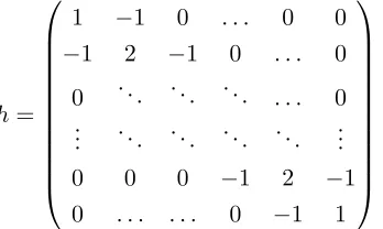
whereHis the Riesz-Representation form of the one dimensional negative Laplacian−∆h given
by
Z
Ω
|∇θ|2 dx= (Hθ, θ), (3.19)
and
H=h⊗I+I⊗h. (3.20)
h=
1 −1 0 . . . 0 0
−1 2 −1 0 . . . 0 0 . .. ... ... . . . 0
..
. . .. ... ... ... ...
0 0 0 −1 2 −1
0 . . . 0 −1 1
.
In summary, the equation of enthalpy on a lattice is written as
En−En−1
λ =−κHβ(E
n) +Bgn, (3.21)
where (Bgn, θ) = (g, θ)Γ. Equation (3.21), is an equation for En, given En−1 and gn. It is nonlinear, since β(E) is nonlinear. The function β(E) is not C1, but semi-smooth. Thus, we use the well-known Semi-smooth Newton method [47, 49] to solve equation (3.21) forEn with the Newton derivative ofβ(E), also see Appendix D.1. So, using the tangent equation
β(E+)∼β0(E)(E+−E) +β(E) (3.22) where
β0(E) =
1
ρc`
E, E > ρL,
1
ρcs
E, E≤ρL,
(3.23)
we obtain the linearization as discrete time iterative algorithm for En Ek−En−1
∆t =−κ H(β
0(E
k−1)(Ek−Ek−1) +β(Ek−1)) +Bgn, E0=En−1, (3.24) whereEk is thek-th iterate. Equation (3.24) is a linear equation forEk, and we can show that
Ek→En.
To write a code for solvingEn, let q= (ρc`, ρcs) be the slopes, then
q(En−En−1) =−κHEn.
So, we have
γn+1−γn
∆t =−κ E
n+1−g. (3.25)
Also, we can write
γn+1−γn
∆t =
q(En+1−En)
∆t (3.26)
Thus, from (3.25) and (3.26), we get
q(En+1−En)
∆t =−κ(E
n+1−En)−κ En−g, (3.27)
which can be written as
(q+ ∆t κ)(En+1−En) = (−κ En−g) ∆t (3.28) Solving equation (3.28) for En+1, we get the iterative algorithm
En+1=En−(q+ ∆t κ)−1(κ En+g) ∆t (3.29) The following is the MATLAB code performing the algorithm discussed above.
for kkk=1:200; T0=Tm*ones(n^2,1)+0.e-5*(E-rhoL/2); q=1e5*ones(n^2,1);
i=find(E(:)>=rhoL); T0(i)=Tm+(E(i)-rhoL)/rho/cL; q(i)=rho*cL;
j=find(E(:)<=0); T0(j)=Tm+E(j)/rho/cS; q(j)=rho*cS; q=spdiags(q(:),0,n^2,n^2);
3.4.1 Numerical Test Examples
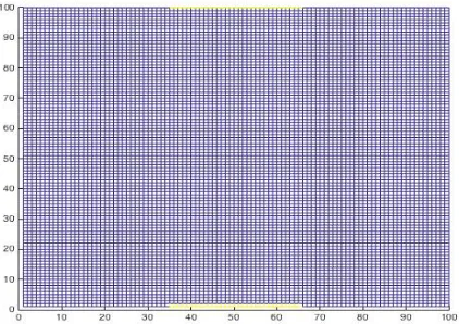
In this section we test the proposed numerical methods for the enthalpy formulation (3.29). The control boundary Γc is given as in Figure 3.2. We first test the algorithm for a forward
Figure 3.2 The control boundary Γc
simulation. We take a constant control g = 5 at Γc and after T = 10 we obtain the splitting
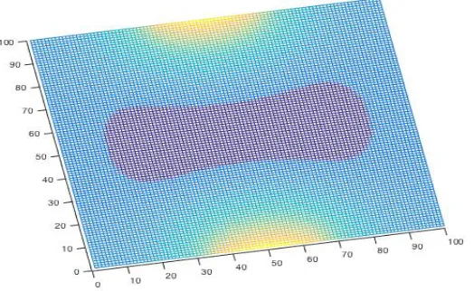
of solid region (blue), depicted in Figure 1.2 in Chapter 1. Time snap-shots of the enthalpy function toward the splitting are shown in Figure 3.3 below. We use
n=100, rho=1.460; dt=.1;
Tm=32; Ts=25; Tl=90;
L=251.21;
cL=3.31; cS=1.76; kL=.59e-3; kS=2.16e-3; rhoL=rho*L.
Next, we present a numerical test for the optimal control problem. The formulation of our numerical test is to achieve the target state, that is the final state at T = 1 of the full horizon problem by the optimal control casted on the half horizon [0, T /2].
First, Figure 3.4 shows the target state. We use the sequential programming method, described in Appendix D.2, and each subproblem of the sequential linearized control problem is solved by the conjugate gradient method, introduced in Appendix D.3. The result of this test is shown in Figure 3.5.
Figure 3.3 Splitting of solid region (blue) by boundary flux
the optimal control on Γc×[0, T /2] show that the geometry is symmetric. Thus, control is
symmetric in the upper and lower portions of Γc. Also, numerical calculations show that the
average heat budget over the half horizon is 4.989 compared to 5 over the full horizon. The MATLAB code for the forward problem and the optimal control problem are given as
rho=1460; rho=rho/1000; dt=.1;
Tm=32; Ts=25; Tl=90;
L=251.21;
cL=3.31; cS=1.76; kL=.59e-3; kS=2.16e-3; rhoL=rho*L;
n=100; m=n-1; e=ones(n,1); h=spdiags([-e 2*e -e],[-1:1],n,n);
h(1,1)=1; h(n,n)=1; h=n^2*h; a=1:n*m; a=a(:);
h=kron(speye(n),h)+kron(h,speye(n));
Figure 3.4 The full horizon target state
T=33*ones(n,n); T(k)=25; T=(speye(n^2)+1.e-3*h)\T(:);
i=find(T(:)>=Tm); E(i)=rho*cL*(T(i)-Tm)+rhoL;
j=find(T(:)<Tm); E(j)=rho*cS*(T(j)-Tm); E=E(:);
g0=zeros(100); g0(1,35:65)=5; g0(end,35:65)=5; g0=n*g0; E0=E;
Q=speye(n^2); u=ones(1,50); QQ=zeros(n^2,20);
for kkk=1:200; T0=Tm*ones(n^2,1)+0.e-5*(E-rhoL/2); q=1e5*ones(n^2,1);
i=find(E(:)>=rhoL); T0(i)=Tm+(E(i)-rhoL)/rho/cL; q(i)=rho*cL;
j=find(E(:)<=0); T0(j)=Tm+E(j)/rho/cS; q(j)=rho*cS; q=spdiags(q(:),0,n^2,n^2);
E=E-q*((q+(kS*dt)*h)\(kS*dt*h*T0-dt*g0(:))); end
E=E0; u=ones(1,50); %we must specify control u=g_{kkk} to compute E
for kkk=1:50; EE(:,kkk)=E; %%%% we must specify control u=g_{kkk}
for k=1:20; T0=Tm*ones(n^2,1)+0.e-5*(E-rhoL/2); q=1e5*ones(n^2,1);
i=find(E(:)>=rhoL); T0(i)=Tm+(E(i)-rhoL)/rho/cL; q(i)=rho*cL;
j=find(E(:)<=0); T0(j)=Tm+E(j)/rho/cS; q(j)=rho*cS; q=spdiags(q(:),0,n^2,n^2);
%%%%% Store the solid index jj=[jj j]; (be careful since j has different length)
Figure 3.5 Half horizon result
%%%% adjoint
R=[]; p=0*E; for kkk=50:-1:1; E=EE(:,kkk);
%% we must have E (initial condition for the horizon)
for k=1:20; T0=Tm*ones(n^2,1)+0.e-5*(E-rhoL/2); q=1e5*ones(n^2,1);
i=find(E(:)>=rhoL); T0(i)=Tm+(E(i)-rhoL)/rho/cL; q(i)=rho*cL;
j=find(E(:)<=0); T0(j)=Tm+E(j)/rho/cS; q(j)=rho*cS; q=spdiags(q(:),0,n^2,n^2);
%%%%% Store the solid index jj=[jj j]; (be careful since j has different length)
E=E-q*((q+(kS*dt/2)*h)\(kS*dt*h*T0-dt*u(kkk)*g0(:))); EEP(:,k)=E; end
Btp=0; for k=20:-1:1; p=(q+(kS*dt)*h)\(q*(p+1.e-2*dt*Q*(EEP(:,k)-Eb)));
Btp=Btp+dt*sum(p.*g0(:)); end; R=[Btp R]; end
R=u+R/n^2; g=-R’; eold=g’*g; d=g; v=0*g;
while eold>ep, E=E0; Ep=0*E; for kkk=1:50; EE(:,kkk)=E; EP(:,kkk)=Ep;
%%%% we must specify control u=g_{kkk}
for k=1:20; T0=Tm*ones(n^2,1)+0.e-5*(E-rhoL/2); q=1e5*ones(n^2,1);
i=find(E(:)>=rhoL); T0(i)=Tm+(E(i)-rhoL)/rho/cL; q(i)=rho*cL;
j=find(E(:)<=0); T0(j)=Tm+E(j)/rho/cS; q(j)=rho*cS; q=spdiags(q(:),0,n^2,n^2);
%%%%% Store the solid index jj=[jj j]; (be careful since j has different length)
Figure 3.6 The resultant optimal control on the half horizon
Ep=q*((q+(kS*dt)*h)\(Ep+dt*d(kkk)*g0(:))); end; end
%%%% adjoint
R=[]; p=0*E; for kkk=50:-1:1; E=EE(:,kkk); Ep=EP(:,kkk);
%% we must have EE, EEP
for k=1:20; T0=Tm*ones(n^2,1)+0.e-5*(E-rhoL/2); q=1e5*ones(n^2,1);
i=find(E(:)>=rhoL); T0(i)=Tm+(E(i)-rhoL)/rho/cL; q(i)=rho*cL;
j=find(E(:)<=0); T0(j)=Tm+E(j)/rho/cS; q(j)=rho*cS; q=spdiags(q(:),0,n^2,n^2);
%%%%% Store the solid index jj=[jj j]; (be careful since j has different length)
E=E-q*((q+(kS*dt)*h)\(kS*dt*h*T0-dt*u(kkk)*g0(:)));
Ep=q*((q+(kS*dt)*h)\(Ep+dt*d(kkk)*g0(:))); EEP(:,k)=Ep; end;
Btp=0; for k=20:-1:1; p=(q+(kS*dt)*h)\(q*(p+1e-2*dt*Q*EEP(:,k)));
Btp=Btp+dt*sum(p.*g0(:)); end; R=[Btp R]; end
%%%%% we claim Lv=R;
%%%%% we claim Ld=R; A=al*I+L (as Av=-R)
Ld=1*d+R’/n^2; al=eold/(d’*Ld); v=v+al*d; g=g-al*Ld; z=g; enew=g’*g;
bt=enew/eold; d=g+bt*d; eold=enew; %k=k+1; E=[E eold];
end
Next, we present the half horizon MATLAB code.
i=find(T(:)>=Tm); E(i)=rho*cL*(T(i)-Tm)+rhoL;
j=find(T(:)<Tm); E(j)=rho*cS*(T(j)-Tm); E=E(:);
g0=zeros(100); g0(1,35:65)=5; g0(end,35:65)=5; g0=n*g0; E0=E;
Q=speye(n^2); u=5*ones(62,25); QQ=zeros(n^2,20);
kmax=25; u=5*ones(62,25); psi=0*E; k=find(abs(Eb)<1000); psi(k)=1;
vv=[]; e0=1e8; for jjj=1:30; E=E0; %we must specify control u=g_{kkk} to compute E
ii=0; for kkk=1:kmax; %%%% we must specify control u=g_{kkk}
g0(1,35:65)=u(1:31,kkk)’; g0(end,35:65)=u(32:62,kkk)’;
for k=1:20; ii=ii+1; T0=Tm*ones(n^2,1)+0.e-5*(E-rhoL/2); q=1e5*ones(n^2,1);
i=find(E(:)>=rhoL); T0(i)=Tm+(E(i)-rhoL)/rho/cL; q(i)=rho*cL;
j=find(E(:)<=0); T0(j)=Tm+E(j)/rho/cS;
q(j)=rho*cS; QQ(:,ii)=q; q=spdiags(q,0,n^2,n^2);
%%%%% Store the solid index jj=[jj j]; (be careful since j has different length)
E=E-q*((q+(kS*dt)*h)\(kS*dt*h*T0-dt*n*g0(:))); end; end; Eb=E;
%%%% adjoint
R=[]; p=psi.*(E-Eb); ii=20*kmax+1; for kkk=kmax:-1:1;
%% we must have E (initial condition for the horizon)
Btp=zeros(62,1); for k=20:-1:1; ii=ii-1; q=spdiags(QQ(:,ii),0,n^2,n^2);
p=(q+(kS*dt)*h)\(q*p); pp=reshape(p,n,n);
Btp=Btp+dt*n*[pp(1,35:65) pp(end,35:65)]’; end; R=[Btp R]; end
R=.000001*u+R/n^2; g=-R(:); eold=g’*g, d=g; if eold >e0; break, end;
v=0*g;e0=eold; gg=g; %(Eb=E===> p=0==>R=0)
%while eold>1.e-0,
for iii=1:3; ii=0; Ep=0*E0; dd=reshape(d,62,25); for kkk=1:kmax;
g0(1,35:65)=dd(1:31,kkk)’; g0(end,35:65)=dd(32:62,kkk)’;
for k=1:20; ii=ii+1;q=spdiags(QQ(:,ii),0,n^2,n^2);
Ep=q*((q+(kS*dt)*h)\(Ep+dt*n*g0(:))); end; end %%%(what we need is to have q)
%%%% adjoint
R=[]; p=psi.*Ep; ii=20*kmax+1; for kkk=kmax:-1:1; %% we must have EE, EEP
Btp=zeros(62,1); for k=20:-1:1; ii=ii-1; q=spdiags(QQ(:,ii),0,n^2,n^2);
p=(q+(kS*dt)*h)\(q*p); pp=reshape(p,n,n);
Ld=.000001*d+R(:)/n^2; al=eold/(d’*Ld); v=v+al*d; g=g-al*Ld; z=g; enew=g’*g,
bt=enew/eold; d=g+bt*d; eold=enew; %k=k+1; E=[E eold];
Chapter 4
Cahn-Hilliard Navier-Stokes System
In this chapter we focus on the phase-field model of separation of two fluids. Our objective is to control the Cahn-Hilliard Navier-Stokes system by the boundary control of the velocity field, i.e. v|∂Ω = u, where Ω is a bounded domain with a sufficiently smooth boundary ∂Ω. Phase separation is considerably involved with a lot of important applications in industry. The main equation that describes the phase separation of a binary fluid mixture is the Cahn-Hilliard equations.
The transport Cahn-Hilliard model can be derived as a gradient flow from an energy as
∂c
∂t +∇ ·J = 0, (4.1)
where cis the concentration of the fluid and J is the diffusional mass flux proportional to the gradient of the generalized chemical potential and the transport as
J =c v−α∇w, (4.2)
whereα >0 is a diffusion coefficient,wis the chemical potential, andvis the transport velocity field. For the material separation of the two-phase system by the Cahn-Hilliard theory, we define the free-energy potential of the concentrationc by
E(c) = Z
Ω (ε
2|∇c(x)| 2+1
εF(c))dx, (4.3)
whereF(c) is the free-energy density of the materials, and ε 2|∇c|
of the interface region. The graph of the transition layer is given in Figure (4.1) below. The
Figure 4.1 The graph of the transition layer
Ginzburg-Landau potential energy corresponds to
F(c) = 1 2(c
2−1)2. (4.4)
Due to the bi-stable potentialF(c), solutions of the equation represent a separation of the two fluids. The term ε
2|∇c(x)|
2 is added to the energy integral to allow smooth transitions between the two stable states of liquids. This term in the energy forms a diffuse (transition) interface between the two separated states with a profile function, i.e.,
c(x) = tanh(√x
2γ), (4.5)
satisfying the stationary differential equation
γ c00(x)−(c2−1)c= 0, (4.6) and hence the width of the interfacial layer is√γ =ε.
The phase separation process conserves the total mass of concentration c, i.e. Z
Ω
so that
d dt
Z
Ω
c dx= 0, (4.8)
The chemical potential wis defined by the variational derivative of the energyE(c). That is,
(w, h) =δE(c)h= lim
t→0
E(c+t h)−E(c)
t . (4.9)
Thus, the chemical potentialw can be written as
w= 1
εF
0(c)−ε∆c. (4.10)
In order to have conservation of mass, the diffusional mass fluxJ satisfies the boundary condi-tion
n·J = 0, along with n· ∇c= 0, (4.11) which prevents the flow of material into or out of the confined volume. For the case n·v = 0, i.e. no normal velocity at∂Ω, and since
∂ ∂νF
0(c) =F00(c)∂c
∂ν, (4.12)
then, the boundary conditions become
∂c ∂ν =
∂
∂νw= 0, on∂Ω, (4.13)
where ∂
∂ν is the outward normal derivative at the boundary ∂Ω. Note that, if divv = 0, then
we have
divJ = div (c v−α∇w) =−α∆w+v· ∇c.
So, we can write the strong form of the transport Cahn-Hilliard equation (4.1) as
∂c
∂t+v· ∇c−α∆w= 0, ∇ ·v= 0. (4.14)
As a consequence, this bi-harmonic flow is the nature of the model of the Cahn-Hilliard system. We have the bi-harmonic diffusion operatorα∆2, with domain ∂c
∂ν = ∂
In summary, the strong form of the normalized transport Cahn-Hilliard system is given by
∂c
∂t +v· ∇c−α∆w= 0, in Ω w=−ε∆c+1
εF
0(c), in Ω
n· ∇c= 0, n·J = 0, on∂Ω
(4.15)
Throughout this thesis, and for the sake of simplicity of our presentation, we set the thickness parameterε= 1 and the conductivity parameter α= 1.
4.1
Weak Formulation of Cahn-Hilliard System
In this section we introduce the weak form of the Cahn-Hilliard equations, and then develop the existence theory for dynamics control in Section (4.4). The weak form of the concentration equation (4.1) inc is given by
( d
dtc, ψ) + (divJ, ψ) = 0, ∀ψ∈H
1(Ω),
which implies, using Green’s formula, that (∂c
∂t, ψ)−(c v− ∇w,∇ψ) = 0, ∀ψ∈H
1(Ω), (4.16)
where we used
(divJ, ψ) = Z
Γ
(n·J)ψ ds−
Z
Ω
J ∇ψ dx.
and the boundary condition n·J = 0. Moreover
(J,∇ψ) = (c v,∇ψ) + (w,∆ψ).
The weak form of the chemical potential equation (4.10) inw is given by (w, ψ) = (−∆c, ψ) + (F0(c), ψ),
which is derived using Green’s formulas as
sincen· ∇c= 0.
4.2
Incompressible Flow by Navier-Stokes Equations
In this section we introduce the basic theory of the incompressible flow governed by Navier-Stokes Equations. The equations can be derived from the laws of conservation of mass and conservation of momentum, given by
∂ρ
∂t + div(ρv) = 0,
(ρv)t+ div(
1 2ρ|v|
2−S) =f,
(4.18)
whereρ=ρ(t, x) is the mass density,v =v(t, x) is the velocity of the fluid over domain Ω∈Rd, and S is the stress tensor defined as
S= 2µε−p I, (4.19)
whereµ is the viscosity, I is the identity matrix, and εis the linear strain defined by
ε= 1
2(∇v+∇v
t), (4.20)
where
εij =
1 2(
∂vi
∂xj
+∂vj
∂xi
). (4.21)
The Navier-Stokes equation can be written as
ρDv
Dt + divS=f, (4.22)
where
divS= ∆v− ∇p, (4.23)
and Dv
Dt is the Lagrangian derivative (or total derivative or material derivative) of the velocity,
given by
Dv Dt = (
∂v
It is the rate change of the velocity along the flow. It comes from taking the time derivative of
v=v(t, x(t)) (a function of two variables, time tand positionx(t), withv(t, x(t)) = dx
dt), d
dtv(t, x(t)) = ∂v
∂t +v· ∇v= Dv
Dt (4.25)
The transport termv· ∇v is taken coordinate-wise, i.e.,
(v· ∇v)j =v· ∇vj. (4.26)
For example, a two dimensional flow v= (v1, v2) in spatial coordinates x1, x2 has
v· ∇v=
v1 ∂v
1
∂x1
+v2 ∂v
1
∂x2
v1 ∂v
2
∂x1
+v2 ∂v
2
∂x2
=
v· ∇v1
v· ∇v2
Substitute equations (4.23)–(4.24) in equation (4.22), we get
ρ(∂v
∂t +v· ∇v) +∇p=µ∆v+f, (4.27)
wherep is the pressure,µis the viscosity of the medium, and f is the applied force vector. Incompressible flow means that the mass density of the fluid remains constant during flow motion, so the state equation can be written as
ρ=ρ(t, x) =ρ0, (4.28)
for some constantρ0. In this case the mass conservation equation (4.18) becomes
divv =∇ ·v= 0. (4.29)
So, the incompressible Navier-Stokes equations are given by
ρ(∂v
∂t +v· ∇v) +∇p=µ∆v+f, ∇ ·v = 0, (4.30)
the Navier-Stokes equations as a force of the form
f =−∇ ·(∇c× ∇c) =−∆c∇c, (4.31) but
−∆c∇c= (w−F0(c))∇c=w∇c− ∇F(c)
and the term ∇F(c) is absorbed into the pressure term. If we assume normalized mass density
ρ, then the strong form of the coupled incompressible Navier-Stokes equations can be written as
∂v
∂t +v· ∇v−µ∆v+∇p=w∇c, ∇ ·v= 0, (4.32)
The Stokes equation is the massless version (i.e. ρ = 0) of the Navier-Stokes equation (4.30), i.e.,
∇p=µ∆v+f, ∇ ·v= 0, (4.33)
4.2.1 Navier Boundary Conditions and Slip Functions
The Navier boundary condition states that the velocity on the boundary is proportional to the tangential component of the normal stress, i.e.
(S·n)τ+β (τ·v−g) = 0 (4.34)
where (S·n)τ is the tangential component of the normal stress, andg is a given function. The
normal stress (S·n)∈L2(0, T;H−1/2(Γ)). Note that if β→ ∞ in (4.34), then we get
τ ·v=g,
and if β= 0, then we have
(S·n)τ = 0.
In the optimal control analysis, we are interested in the slip boundary conditions, i.e.
τ ·v=g1,
n·v=g2,
4.2.2 Weak Formulation of Navier-Stokes Equations
In this section we introduce the weak form for the velocityv of the momentum equation (4.32). The weak form of the velocity is based on the definition of the tri-linear form b(v, w, φ). We start by introducing the standard divergence-free spaces
V0 ={v ∈H01(Ω)d:∇ ·v= 0}, and
V ={v∈H1(Ω)d:∇ ·v= 0}.
LetH0 and H be the completion ofV0 andV with respect toL2(Ω)d, respectively, i.e.
H0={v∈L2(Ω)d:∇ ·v= 0, n·v= 0, on∂Ω}, and
H={v∈L2(Ω)d:∇ ·v= 0}.
First, we define the tri-linear formb:V ×V ×V0→Rfor the convictive term by
b(v, w, φ) =hv· ∇w, φi= Z
Ω
(v· ∇w)·φ dx.
It can be shown that the trilinear form bsatisfies the following properties (a)b(v, w, φ) +b(v, φ, w) = 0, provided that
divv= 0, and (n·v)(w·φ) = 0, on Γ.
(b)|b(v, w, φ)| ≤ |v|L4 |∇w|L2 |φ|L4 ≤M |v|V |∇w|V |φ|V0.
(c)|b(v, w, φ)| ≤M1 |v|1L/22 |v|
1/2
V |φ|
1/2
L2 |φ|
1/2
V0 |w|V in 2-D.
(d)|b(v, w, φ)| ≤M1|v|1L/24|v|
3/4
V |φ|
1/4
L2 |φ|
3/4
V0 |w|V in 3-D.
The weak form of the Navier-Stokes equations can be derived from (4.22), as (ρDv
which can be written using (4.24), as
(∂v
∂t, φ) + (v· ∇v, φ)−(divS, φ) = (w∇c, φ), ∀φ∈V0, (4.37)
where
(divS, φ) = Z
∂Ω
(n·S)φ ds−
Z
Ω
S:∇φ dx
where we used the Frobenius product defined as Z
Ω
S :∇φ dx=X
i,j
(Sij)(∇φij) = (S,∇φ),
Using the definition of the Stress tensor, we can write
(S,∇φ) = (2µε−p I,∇φ) = 2µ(ε,∇φ) + (p I,∇φ) = 2µ(1
2(∇v+ (∇v)
t),∇φ) + (p,∇φ).
The term (p,∇φ) vanishes, since φ∈V0 and
(∇p, φ) = Z
Ω
∇p φ dx= Z
Γ
(n·φ)p ds−
Z
Ω
pdivφ dx= 0
since, n·φ= 0 and divφ= 0. Thus,
(S,∇φ) =µ(∇v+ (∇v)t,∇φ),
where ∇v= ∂v1 ∂x1 ∂v1 ∂x2 ∂v2 ∂x1 ∂v2 ∂x2 and
2µ ε=
µ∂v1 ∂x1
+µ∂v1 ∂x1
µ∂v1 ∂x2
+µ∂v2 ∂x1
µ∂v2 ∂x1
+µ∂v1 ∂x2
µ∂v2 ∂x2
and ∇φ= ∂φ1 ∂x1 ∂φ1 ∂x2 ∂φ2 ∂x1 ∂φ2 ∂x2
So, since divv= 0, we have
(S,∇φ) =µ(∇v,∇φ).
Thus, the weak form of the coupled Navier-Stokes equation can be written as ( d
dtv, φ) +b(v, v, φ) +µ(∇v,∇φ) = (w∇c, φ), ∀φ∈V0. (4.38)
In summary, the weak form of the coupled system of Cahn-Hilliard Navier-Stokes system can be written as
(d
dtv, φ) +b(v, v, φ) +µ(∇v,∇φ) = (w∇c, φ), ∀φ∈V0
(d
dtc, ψ1)−(c v− ∇w,∇ψ1) = 0, ∀ψ1∈H
1(Ω)
(∇c,∇ψ2) + (F0(c), ψ2) = (w, ψ2), ∀ψ2 ∈H1(Ω).
(4.39)
4.3
Sharpened and Obstacle Ginzburg-Landau Potential
Compared to the weak form given by (4.39), the strong form of the normalized equation of Cahn-Hilliard Navier-Stokes system on Ω can be written as
d
dtv+v· ∇v− ∇ ·(µ(c)∇v) +∇p=w∇c, ∇ ·v= 0. in Ω, v|∂Ω =u, d
dtc+v· ∇c−α∆w= 0, in Ω w=−∆c+Fβ0(c), in Ω
n· ∇c= 0, n·J = 0, on∂Ω