ABSTRACT
PANDIAN, MANI BHARATHI. Optimal Resource Allocation in Heterogeneous Networks. (Under the direction of Dr. Mihail L. Sichitiu and Dr. Huaiyu Dai.)
©Copyright 2014 by Mani Bharathi Pandian
Optimal Resource Allocation in Heterogeneous Networks
by
Mani Bharathi Pandian
A dissertation submitted to the Graduate Faculty of North Carolina State University
in partial fulfillment of the requirements for the Degree of
Doctor of Philosophy
Computer Engineering
Raleigh, North Carolina 2014
APPROVED BY:
Dr. Brian L. Hughes Dr. Wenye Wang
Dr. Mihail L. Sichitiu Co-chair of Advisory Committee
Dr. Huaiyu Dai
DEDICATION
BIOGRAPHY
ACKNOWLEDGEMENTS
I express my deepest gratitude to my advisor Dr. Mihail L. Sichitiu. His tenacious support and unwavering faith in my abilities were the sustaining forces for me throughout the development of this doctoral dissertation. I most enjoyed the long discussions with him which often led to key insights and ideas. Above all, he has been always patient, caring, forgiving, and encouraging in times of uncertainty and difficulties. I couldn’t ask for more in an advisor. I am very grateful to my co-advisor Dr. Huaiyu Dai, for his constant guidance, encouragement, and for many motivating discussions during the weekly meetings. I sincerely thank Dr. Dai for the opportunity to collaborate and for his excellent guidance during my job hunt.
I express my sincere appreciation to all my committee members: Dr. Brian Hughes, Dr. Wenye Wang and Dr. David Thuente, for their comments, critique and suggestions that have greatly improved my research and the quality of this dissertation. I thank Dr. Rudra Dutta for the opportunity to work on the CentMesh Project, and for his guidance and direction.
I am deeply indebted to the National Science Foundation (NSF) and Graduate Student Support Plan (GSSP) for the financial support. I am very thankful to Dr. Michael Devetsikiotis, Ms. Elaine Hardin, Ms. Cailan Mang, and the ECE Graduate Office for all their help and support. My sincere thanks to Mr. Marhn Fullmer for his support and help in ECE470, ECE575, ECE775, and the CentMesh project.
I thank my awesome lab-mates and friends for their company, advise, and help: Junbum, Vineet, Vishwesh, Jangeun, Chen, Yongchul, Heewon, Anand, Fengyuan, Hong, Jenn, Har-ish, Scott, Christina, Lopa, Yun, and Kostas; My ex-flatmates Mandar, Jay, Sachin, Varit, Prashanth, Ameya, Allen, Praveen, Devesh, Srikanth, Abhishek, and Sravan. Thank you Man-dar for all the advise and help during the application process and my first year at NCSU.
I thank my mom, dad, and sister for their infinite support throughout everything. I am eternally indebted to them for all their sacrifices and for raising us in an intellectually stimu-lating environment. Thank you Babu uncle for your genuine care - you are always my “go to” person and you give the best advice. To my most special teacher, Mrs. Nawathe, words cannot express the debt I feel for the time you sacrificed to teach me Hindi for 8 straight years. On a concluding note, the quote below is dedicated to the many people who have helped me through the years. Thank You.
“There is no such thing as a ‘self-made’ man. We are made up of thousands of others. Everyone who has ever done a kind deed for us, or spoken one word of encouragement to us, has entered into the make-up of our character and of our thoughts.”
TABLE OF CONTENTS
LIST OF TABLES . . . vii
LIST OF FIGURES . . . .viii
Chapter 1 Introduction . . . 1
Chapter 2 Background and Related Work . . . 9
2.1 Related Work . . . 9
2.2 Two-Player Cooperative Games . . . 11
2.2.1 Nash Solution . . . 12
2.2.2 Raiffa Solution . . . 14
2.2.3 Utilitarian Solution . . . 15
2.2.4 Egalitarian solution . . . 16
Chapter 3 Optimal Resource Allocation in IEEE 802.11 Based Wireless Local Area Networks. . . 19
3.1 WLAN Model for Time Fairness . . . 23
3.2 WLAN Model for Throughput Fairness . . . 27
3.3 Performance Evaluation . . . 28
3.3.1 Performance Evaluation with Time Fairness Constraints . . . 28
3.3.2 Performance Evaluation with Throughput Fairness Constraints . . . 30
3.4 Support for Downlink Traffic . . . 30
3.5 Accounting for the Effects of Inter-Cell Contention . . . 32
3.6 Protocol Design . . . 34
3.7 Conclusion . . . 34
Chapter 4 CCRN Framework for Single AP WLAN . . . 36
4.1 System Model . . . 38
4.2 Closed-Form Expression for the Bargaining Set . . . 40
4.2.1 Under Time Fairness Constraint . . . 40
4.2.2 Under Throughput Fairness Constraint . . . 41
4.2.3 Validation . . . 43
4.3 CCRN Scheme . . . 44
4.3.1 CCRN Under Time Fairness . . . 44
4.3.2 CCRN Under Throughput Fairness . . . 49
4.4 Performance Evaluation . . . 50
4.5 Conclusion . . . 53
Chapter 5 CCRN Framework for Multi-AP WLANs . . . 54
5.1 System Model . . . 56
5.2 CCRN Framework . . . 58
5.2.3 Bargaining Problem . . . 63
5.2.4 Channel Access . . . 64
5.2.5 CCRN Protocol . . . 65
5.3 Support for Downlink . . . 65
5.3.1 User Association Algorithm . . . 66
5.3.2 Channel Contention Algorithm . . . 67
5.4 Performance Evaluation . . . 67
5.4.1 Simulation Setup . . . 67
5.4.2 User-AP Association Control . . . 68
5.4.3 Linear Bargaining Set . . . 69
5.4.4 CCRN Framework . . . 70
5.5 Conclusion . . . 74
Chapter 6 Optimal Resource Allocation in LTE-Advanced Heterogeneous Net-works with eICIC . . . 76
6.1 Proportional Fairness in HetNets . . . 81
6.1.1 Relaxed Optimization Problem . . . 84
6.1.2 The Rounding Method . . . 85
6.2 Greedy Association Algorithm . . . 87
6.3 Performance Evaluation . . . 90
6.3.1 Simulation Parameters . . . 90
6.3.2 Results . . . 92
6.4 Conclusion . . . 98
Chapter 7 Future Work . . . 99
7.1 CCRN Scheme for Heterogeneous Networks . . . 99
7.2 Cooperative Heterogeneous Cellular Networks . . . 100
References. . . .103
Appendix . . . .110
LIST OF TABLES
Table 3.1 Notations used throughout this chapter. . . 20
Table 3.2 Parameters used to obtain numerical results. . . 21
Table 3.3 ParametersTslot,Tc,η andζfor 802.11 a/b/g/n.. . . 25
Table 5.1 System parameters in the proposed CCRN scheme. . . 71
Table 6.1 CSB per pico BS obtained using GPF algorithm averaged over 50 independent network realizations. . . 97
Table 6.2 Optimality gap of the GPF algorithm for different pico BS transmit powers and user density. . . 97
Table 7.1 Achievable throughput for the wireless subscribers when being serviced by the base station of their own provider. . . 100
LIST OF FIGURES
Figure 1.1 CCRN for Single AP WLAN: Network diagram showing the base station (BS) of the primary network, the access point (AP) of the secondary network, and the primary and secondary users (PUs and SUs) in the range of the AP (a) before, and (b) after spectrum sharing under CCRN framework. . . 4 Figure 1.2 Illustration of an enterprise WLAN after spectrum leasing via CCRN scheme;
network diagram showing the BS of the primary network, the APs of the secondary network, the centralized controller, and the primary and secondary users (PUs and SUs) in the range of the enterprise WLAN and the BS. . . . 5 Figure 1.3 Network diagram showing the interference graph of the APs in the network
(a) before, and (b) after spectrum sharing under CCRN framework. In the interference graph, two APs are connected only if they are within each other’s carrier sensing range. The number on each AP represents the total number of co-channel APs that interfere with the AP under consideration. . . 6 Figure 1.4 A LTE heterogeneous network with a macro base station (BS) and two pico
BSs. The macro BS is muted when User 1 communicates with Pico BS 1. User 2 communicates with the macro BS and User 3 communicates with the Pico BS 2, where both the transmissions are scheduled simultaneously. . . 7 Figure 1.5 A heterogeneous network implementing CCRN scheme. The heterogeneous
network comprising an isolated AP, an enterprise WLAN operating in the unlicensed (e.g. 2.4 GHz) and leased (e.g. 3.5 GHz) bands, pico BS operating in the leased (e.g. 3.5 GHz) band, and a pico BS operating in the licensed band (e.g. 700 MHz) and employing eICIC scheme. . . 8 Figure 2.1 Graphical representation of the Nash bargaining solution for linear
bargain-ing sets. . . 12 Figure 2.2 Relationship between the Nash bargaining solution and the rectangular
hy-perbola. . . 13 Figure 2.3 An example where Nash bargaining solution is controversial, and where
Raiffa’s solution is more acceptable. . . 14 Figure 2.4 Utilitarian solution for linear bargaining sets with slope−1+, 1, and,−1−
respectively. . . 15 Figure 2.5 Comparing Egalitarian solution and Nash solution for linear bargaining sets. 16 Figure 3.1 An IEEE 802.11 enterprise wireless local area network with access points
(APs) and users. . . 19 Figure 3.2 The rate region of an 802.11b multi-rate WLAN with two nodes where the
bit rate of node 1 is 5.5 Mbps and node 2 is 11 Mbps. Each point in the rate region represents the throughput allocation for a certain chosen channel access probability by the users. . . 22 Figure 3.3 Performance comparison of the five MAC algorithms under time fairness:
Figure 3.4 Proportional time allocation in a 802.11b WLAN with two traffic classes: (a) Aggregate throughput per class vs. number of nodes under; (b) short-term fairness of the channel occupancy. . . 30 Figure 3.5 Proportional throughput allocation in a 802.11b WLAN with two traffic
classes: (a) Aggregate throughput per class vs. number of nodes under; (b) short-term fairness of the channel occupancy. . . 31 Figure 4.1 Network diagram showing the base station (BS) of the primary network, the
access point (AP) of the secondary network, and the primary and secondary users (PUs and SUs) in the range of the AP (a) before, and (b) after spectrum sharing under CCRN framework. . . 37 Figure 4.2 The bargaining set B, bargaining point (Xpb, Xsb) and disagreement point
(Xpd, Xsd) for the CCRN problem without (a), and with (b) fairness constraint (timeorthroughput) coupled with the use of the optimized access probabilities. 38 Figure 4.3 Comparison of the optimal aggregate throughput of class1 and class2 with
the approximated linear equation under (a) time fairness, and (b) throughput fairness constraints. . . 43 Figure 4.4 Graphical representation of the bargaining problem along with the Nash
solution when the access probability for the users and AP inline 3of Algo-rithms 2 and 3 are obtained using the (a) the optimal WLAN model in (3.17) of Chapter 3, and (b) the approximate WLAN model in (3.29) of Chapter 3. 48 Figure 4.5 Percentage improvement in the aggregate throughput of the primary and
secondary users while varying the number of primary users and holding the number of secondary users constant (ns=10) for (a) uniform, and (b)
clus-tered placements. . . 51 Figure 4.6 Percentage improvement in the throughputs of the primary and secondary
users while varying the initial aggregate throughput of the primary users for (a) uniform, and (b) clustered placements. . . 52 Figure 5.1 An enterprise WLAN showing the base station (BS) of the primary network,
with access points (APs) of the secondary network, and the primary and secondary users (PUs and SUs) in the range of the enterprise WLAN and the BS; (a) before spectrum leasing, all primary users associate with their BS while the secondary users associate with their APs, (b) after spectrum leasing, all primary and secondary users associate with the APs in the WLAN. 55 Figure 5.2 Illustration of an enterprise WLAN after spectrum leasing via CCRN scheme;
network diagram showing the BS of the primary network, the APs of the secondary network, the centralized controller, and the primary and secondary users (PUs and SUs) in the range of the enterprise WLAN and the BS. . . . 57 Figure 5.3 The bargaining set B, bargaining point (Xpb, Xsb) and disagreement point
(Xpd, Xsd) for the CCRN problem without (a), and with (b) fairness constraint. 57 Figure 5.4 An example of AP and user distribution in the simulation: (a) Homogeneous,
Figure 5.5 Per user throughput comparison between GreedyAP and SSF association schemes for user weights wp = 1, ws= 10 for a randomly generated (a)
uni-form and, (b) hotspot topology with the number of primary users, secondary users, and APs set to 250,150,and 15 respectively. . . 69 Figure 5.6 The coefficient of determination (also known as R-squared) and the
nor-malized root mean square error (RMSE) between the (Xp, Xs) computed
for the 40 different user weights pair and the estimated linear bargaining set Xp+Xs =h for 100 randomly generated (a) uniform and, (b) hotspot
topologies. . . 70 Figure 5.7 Percentage increase in the throughput of (a) primary, and (b) secondary
network when the number of primary users is varied between 50 and 300. . . 71 Figure 5.8 Percentage increase in the throughput of (a) primary, and (b) secondary
network when the number of secondary users is varied between 50 and 300. . 72 Figure 5.9 (a) Aggregate throughput of the enterprise WLAN before and after
spec-trum leasing; Percentage increase in the throughput of (a) primary, and (b) secondary network when the number of APs is varied between 15 and 30. . . 73 Figure 5.10 Percentage increase in the throughput of (a) primary, and (b) secondary
network when the primary network throughput before cooperation, Xpd, is varied between 33.4 Mbps and 346 Mbps. . . 74 Figure 5.11 Percentage increase in the throughput of (a) primary, and (b) secondary
network when the number of leased channels (licensed channels) is varied between 1 and 5. . . 75 Figure 6.1 A heterogeneous cellular network with one macro base station (BS) and two
overlaid pico BSs. . . 77 Figure 6.2 (a) A simple topology with a macro BS and three pico BSs at 300 m, 1500
m, and 2400 m respectively. (b) The achievable link bit rate for a users at different distances from the macro BS and the pico BSs. The transmit power for the macro and pico BSs are set to 46 dBm and 30 dBm, respectively. . . . 78 Figure 6.3 (a) The HetNet in Fig. 6.1 with Users 1, 2, and 3 as the only active users.
Figure 6.4 User and BS associations obtained with different eICIC schemes: (a) the lo-cation of the macro and pico BSs, (b) location of the users. For the net-work in (a) and (b), the user and BS association obtained by (c) solv-ing (RELAXOPT), (d) CPF in Algorithm 5, (e) GPF in Algorithm 6, and (f) the best SSF scheme (CSB of 15 dB and ABS airtime fraction of 0.3). For the sake of simplicity, we only show the users that receive airtime from a pico BS. The users with association not shown are all associated with the macro BS. The lines denote users scheduled on the ABS slots; denotes a user fractionally associated with both the macro and a pico BS; denotes a user scheduled over both ABS and Non-ABS slots of a pico BS; ×denote users exclusively scheduled on the Non-ABS slots; denote users exclusively scheduled on the BS slots. . . 93 Figure 6.5 Per-user throughput for the different eICIC schemes evaluated in Fig. 6.4.
The users are sorted in the increasing order of their throughput. . . 95 Figure 6.6 Per-user throughput for the different eICIC schemes averaged over 50
inde-pendent network realizations. The users are sorted in the increasing order of their throughput. . . 96 Figure 7.1 A heterogeneous network implementing CCRN scheme. The heterogeneous
network comprising an isolated AP WLAN, an enterprise WLAN operating in the unlicensed (e.g. 2.4 GHz) and leased (e.g. 3.5 GHz) bands, pico BS operating in the leased (e.g. 3.5 GHz) band, and a pico BS operating in the licensed band (e.g. 700 MHz) and employing eICIC scheme. . . 99 Figure 7.2 An example with two cellular (heterogeneous) network providers and four
wireless subscribers for each provider, where the subscribers are being ser-viced by the base station of their own provider. . . 101 Figure 7.3 An example with two cellular (heterogeneous) network providers and four
wireless subscribers for each provider, where the subscribers are being ser-viced by the best station available. . . 102 Figure A.1 Two real branches of the Lambert W function. Dashed line: W−1(z) defined for
Chapter 1
Introduction
Mobile data offload to small cell technology such as WiFi or picocell provides a compelling solution for mobile operators who want to relieve the strain on their core networks. Compared to cellular macrocells, small cells provide increased spectrum reuse in the coverage area, and a higher signal to noise ratio in the cell (hence superior link bit rate for its users). Furthermore, the reduced transmission times enabled by the superior link bit rates in the small cells directly translate into battery power saving for the user devices. WiFi hotspots operate in the unlicensed bands and suffer from severe interference due to scarce spectrum availability. On the other hand, macrocells and femtocells require the use of the same costly and scarce licensed spectrum and suffer from co-site interference problems.
To unlock new spectrum for small cell technology, a new regulatory spectrum sharing frame-work [1] is being proposed by the Federal Communications Commission (FCC), where non-mobile incumbent owners, such as military who do not use their spectrum at all times and locations are allowed to grant exclusive access of their spectrum to mobile operators in regions where there is no incumbent activity. Recently, FCC and the US Federal government have iden-tified the 3550-3650 MHz band [2] (3.5 GHz Band), currently utilized for military and satellite operations localized to the U.S. coastline, as an ideal spectrum band for shared use with mobile operators for small cell operations. The European Commission is working on a similar pro-posal in the 2.3-2.4 GHz band that has very localized incumbent military telemetry use. Such a spectrum sharing approach regime can potentially unlock more than 100 MHz of high-quality spectrum, specially in higher spectrum bands (>2 GHz) that are ideal for small cells.
across the U.S. The WSDs learn of white spaces availability at their respective location using a location-based query to the central white space spectrum database. Due to this requirement, WSDs are also referred to as “database-driven cognitive radios” [4] [5]. Recent success with WSDs has prompted the FCC to create a similar database-driven dynamic spectrum access system for spectrum sharing in the 3.5 GHz band as well (see [6] for a 3.5 GHz transceiver that can negotiate Quality of Service (QoS) guarantees with spectrum databases). Also, use of database-driven cognitive radios will expedite spectrum sharing in real-world networks as they circumvent the highly challenging spectrum sensing feature of traditional cognitive radios.
To expedite spectrum sharing in small cells, FCC in its recent ruling [7] has eliminated spectrum sensing as a requisite for cognitive radio devices. Instead, FCC mandates that de-vices learn of spectrum availability at their respective locations from an external source such as a location-based query to the database of the incumbent, for example the Google Spectrum Database [3]. Devices with such “cognitive” or “frequency-agile” transceivers are regarded as the main enabler of spectrum sharing in small cell technology. Although, spectrum leasing sim-plifies commercial deployment and promotes better spectrum utilization, developing a workable pricing model between the primary network (owner of the spectrum) and the secondary network (beneficiary of the leased spectrum) is not trivial. To expedite spectrum leasing in real-world deployments, researchers have recently advocated for schemes that employ spectrum leasing, not necessarily on the basis of fees or charge, but in return for improved quality-of-service of the primary network via cooperation with secondary network. One such proposal is the new cog-nitive radio paradigm in [8] termed Cooperative Cognitive Radio Networks (CCRNs). CCRNs exploit cooperative diversity in cognitive radio networks by combining cooperative communi-cation [9], a physical layer technology, and the spectrum leasing feature enabled by cognitive radios. In CCRNs, the primary users select a set of secondary users (which have better channel conditions) to relay the primary traffic cooperatively, and in return the secondary users are granted channel access opportunities in the licensed (leased) spectrum. This way, CCRNs avoid the following two major challenges with spectrum sharing in present day networks:
spectrum sensing feature in cognitive radios,
creating a workable pricing model between the primary and secondary networks.
Instead, CCRNs promote spectrum leasing through the use of database-driven cognitive ra-dios and employ non-monetary rewards to enable cooperation between primary and secondary networks.
using other special orthogonal schemes [15]. A random access scheme is presented in [16], where secondary users access the spectrum using slotted Aloha. However, none of the CCRN schemes are directly applicable to the two most widely deployed wireless networks:
1. IEEE 802.11 based Wireless Local Area Networks (WLANs), and,
2. LTE Advanced Heterogeneous Networks (HetNets) comprising a macro and multiple pico base stations (BSs) which are co-deployed and use the same operating channel.
In our work, we propose an implementation of the CCRN framework for WLANs and LTE Ad-vanced Heterogeneous Networks. In the following sections, we briefly outline the contributions of this dissertation.
In Section 2, we present a brief literature survey on the works that advocate the use of the CCRN framework. We also outline the various bargaining solutions, including the Nash solution, which can be employed in our proposed CCRN schemes.
Achieving fairness and efficient use of resources (channel time or achievable throughput) are essential in WLANs. For this reason, in the proposed CCRN scheme, we impose either a weighted time or a weighted throughput fairness constraint, where the primary and sec-ondary users are assigned separate traffic classes. Under the weighted time fairness constraint, users share their channel occupancy time in proportion to their assigned weights; while under weighted throughput fairness constraint, the users share their achievable throughput in propor-tion to their assigned weights. Our CCRN scheme for WLANs require an IEEE 802.11 DCF like contention based channel access mechanism that will achieve the chosen fairness constraint (weighted time or weighted throughput). In Chapter 3, we propose WLAN models for our CCRN scheme that is based on the recent work in [17]. The WLAN model in [17] calculates an optimal fixed contention window for each contending station in an IEEE 802.11 multi-rate WLAN to jointly achieve aggregate WLAN throughput maximization and time fairness (equal channel occupancy time for all stations). To fit our CCRN needs, the WLAN model in [17] is extended in the following directions in Chapter 3:
1. to support weighted time or weighted throughput fairness constraint among stations in the WLAN, and
2. to support both uplink as well as downlink traffic.
INTERNET
SU PU
SU
Licensed Spectrum (LTE)
Unlicensed Spectrum
(WLAN)
BS AP
PU
(a)
INTERNET
SU PU
PU SU
Leased Spectrum (WLAN-1)
Unlicensed Spectrum (WLAN-2)
BS AP
(b)
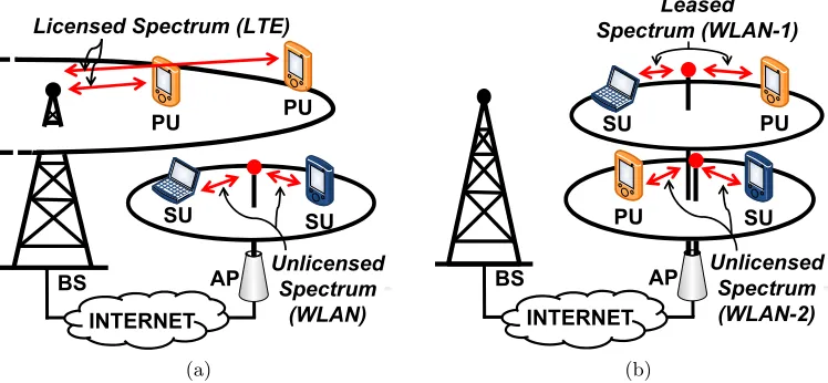
Figure 1.1: CCRN for Single AP WLAN: Network diagram showing the base station (BS) of the primary network, the access point (AP) of the secondary network, and the primary and secondary users (PUs and SUs) in the range of the AP (a) before, and (b) after spectrum sharing under CCRN framework.
experiments, we show that the loss in optimality when using the approximate WLAN model is negligible.
In Chapter 4, we propose the CCRN framework for single AP WLANs. As shown in Fig. 1.1, in the proposed CCRN scheme, the mobile operator leases a channel from the licensed spectrum band to a privately owned WiFi AP, and in return, the mobile operator leverages the AP as cooperative relays to offload its Internet traffic. The cooperation between the primary (cellular) and secondary (WLAN) networks is analyzed using a two-player bargaining game where the utility function for the players are their respective aggregate network throughputs. We show that under fairness and optimal throughput constraints, the bargaining set for the bargaining game is a straight line whose slope only depends on the bit rates of the users. The optimal resource allocation that ensures efficiency as well as fairness between players is provided by the Nash bargaining solution. Calculating the Nash bargaining solution for linear bargaining set is trivial and the proposed CCRN scheme determines the distribution of the users in the two WLAN and the traffic weights for the users at the Nash solution. The proposed computationally inexpensive WLAN model in Chapter 3 then calculates the contention window for each user that would result in the operating point of the system close to the Nash solution. The simulation results verify the optimality of the operating point as well as quantify the benefits of employing the CCRN scheme in single AP WLANs.
BS PU AP SU
INTERNET
ETHERNET
CONTROLLER
2.4 GHz Ch1
2.4 GHz Ch6 3.5 GHz Ch1 4G LTE at 700 MHz
Figure 1.2: Illustration of an enterprise WLAN after spectrum leasing via CCRN scheme; network diagram showing the BS of the primary network, the APs of the secondary network, the centralized controller, and the primary and secondary users (PUs and SUs) in the range of the enterprise WLAN and the BS.
can substantially increase the throughput of the cellular users even with fewer leased channels. The throughput improvement for the WLAN users (secondary users) is not as spectacular primarily because they have relatively higher throughputs even before spectrum leasing.
0 50 100 150 200 250
0 50 100 150 200 250 1 3 4 3 1 6 6 2 3 3 6 2 3 4 4 3 1 2 3 4 6 3 3 4 7 2 8 2 6 4 2 5 4 3 3 (a)
0 50 100 150 200 250
0 50 100 150 200 250 1 0 2 2 0 1 3 0 0 0 2 0 0 0 1 1 1 1 2 1 2 0 1 2 2 0 2 0 3 0 1 2 2 1 2 (b)
Figure 1.3: Network diagram showing the interference graph of the APs in the network (a) before, and (b) after spectrum sharing under CCRN framework. In the interference graph, two APs are connected only if they are within each other’s carrier sensing range. The number on each AP represents the total number of co-channel APs that interfere with the AP under consideration.
macro BS transmissions and therefore cannot communicate with the pico BS. To protect cell-edge users such as User 1 in Fig. 1.4, LTE Advanced introduced a scheme named enhanced Inter Cell Interference Coordination (eICIC). In the eICIC scheme, the macro BS is muted during the slots where the pico-cell edge users are scheduled. With reduced macro interference in the muted slots, pico-cell edge users can communicate error free with the pico BS. Intuitively, a larger number of muted slots will improve throughput of pico cell users at the expense of reduced airtime for the users of the macro BS. Therefore, determining the optimal user-BS (macro or pico BS) association, airtime for each user, and the number of muted slots are essential to the performance of the HetNet. In Chapter 6, we develop algorithms for eICIC based LTE-HetNets to optimize the number of muted slots, per-user throughput, and pico BS utilization, while accounting for all the network parameters such as the link bit rate of the users from their reachable BSs, the macro BS to pico BS interference, and the network topology.
User 1
User 3 User 2
Pico BS 1
Pico BS 2 Macro BS
SINR from pico BS strongest
SINR from macro BS strongest
Figure 1.4: A LTE heterogeneous network with a macro base station (BS) and two pico BSs. The macro BS is muted when User 1 communicates with Pico BS 1. User 2 communicates with the macro BS and User 3 communicates with the Pico BS 2, where both the transmissions are scheduled simultaneously.
is left as future work, but all the necessary tools required for drafting the scheme have already been developed in this work. Specifically, the system model for the CCRN scheme for HetNets is along similar lines to the CCRN problem formulation for enterprise WLANs in Chapter 5.1. The optimal resource allocation in HetNets is achieved by employing the algorithms for WLANs and LTE networks proposed in Chapter 3 and Chapter 6, respectively.
Macro BS
Enterprise WLAN Pico BS
with LTE eICIC
Pico BS
with LTE eICIC with LTEPico BS Single AP
WLAN 3.5 GHz
band
2.4 GHz band
2.4 GHz band 3.5 GHz
band
700 MHz band
Chapter 2
Background and Related Work
2.1
Related Work
order n polynomial which renders it unsuitable for real-time implementation in the driver of a commodity wireless card. In Chapter 3, we combine the work of [21] and [17], and present a computationally inexpensive WLAN model for computing the optimal contention window for each node under time and throughput fairness constraints. We further extend our WLAN models to also support service differentiation (or quality of service (QoS)) in WLANs. The binary exponential backoff mechanism of DCF causes short-term unfairness where the collided nodes choose long backoffs with higher probability, thereby allowing other nodes to benefit from increased channel access. We eliminate the problem of short-term unfairness by disabling the exponential backoff mechanism of DCF, i.e., the maximum contention window size (CWmax)
is always fixed and is not doubled after a collision. The proposed WLAN model calculates the appropriate maximum contention window size for each node so that they jointly satisfy the fairness constraint while maximizing throughput.
tiple independent data streams, the need for phase 3 is eliminated where now the secondary users cooperatively relay the primary traffic in phases 1 and 2 while obtaining spectrum access opportunities for their own traffic. While [13] leverages the degrees of freedom (DoFs) offered in the spatial domain, [15] exploits the DoFs provided by the orthogonal dimensions in quadrature phase shift keying (QPSK). The secondary users employ in-phase binary phase shift keying (I-BPSK) to relay the primary traffic and use the quadrature BPSK (Q-(I-BPSK) to transmit their own traffic. A two-phase FDMA scheme is proposed in [12], where the primary users grant secondary users exclusive access to a portion of their spectrum in exchange for cooperation. As far as we know, no CCRN framework has been proposed for:
1. WLANs employing contention based access schemes such as IEEE 802.11 DCF, and, 2. LTE Advanced Heterogeneous Networks employing eICIC scheme.
In Chapters 4 and 5, we present the CCRN framework for IEEE 802.11 based multi-rate WLANs.
The eICIC proposal is relatively new for LTE Heterogeneous networks. In [24], the authors present a very good introduction to the concept of eICIC in LTE HetNets. An excellent survey on eICIC and the motivation behind eICIC proposal in LTE standards is presented in [25]. The authors in [26] have developed algorithms for optimal configuration of eICIC parameters based on the actual network topology, propagation data, traffic load etc. Simulation results show significant gains in throughput is achievable when the base station scheduling and the user association are both jointly optimized. The work in [27] show the trade-off between proportional fairness and optimizing the time taken to deliver data destined for all users in the network. The authors in [27] claim that optimizing the time taken to deliver user data is a more appropriate fairness criteria for eICIC based LTE networks.
2.2
Two-Player Cooperative Games
In this section we present a brief survey of the various bargaining solutions from the literature on game theory. Bargaining games, also known as cooperative games, are a branch of game theory where:
players have the possibility of agreeing on a rational joint plan of action; there is a conflict of interest about agreements among players;
no agreement may be imposed on any player without that player’s consent.
process: a sequential game involving a series of offers and counteroffers to arrive at an equilib-rium. Nash [28] describes the axiomatic approach as “one states as axioms several properties that it would seem natural for the solution to have and then one discovers that axioms actually determine the solution uniquely.” Thus the axiomatic approach abstracts away the details of the process of bargaining and uses the axioms to narrow down the search to a single solution point. Nash [28], Raiffa-Kalai-Smorondinsky [29] (henceforth, Raiffa’s solution), Egalitarian [30] and the Utilitarian rule [31] are some of the well-known axiomatic solutions for the bargaining prob-lem. A thorough treatment of other bargaining solutions in the literature can be found in [32], and in this section we briefly discuss the axioms of Nash, Raiffa, Egalitarian and Utilitarian solutions.
1
1 2
2
0,0
′
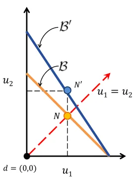
Figure 2.1: Graphical representation of the Nash bargaining solution for linear bargaining sets.
A two player bargaining game is defined by a pair (B, d), where the plane B ⊂ R2+ is a
compact and convex set representing the feasible set of utilities (u1, u2) of the two players. The
bargaining rangeBd is the set of points ofB dominatingd,Bd={(u1, u2)∈ B |u1 ≥d1, u2 ≥
d2}, where d = (d1, d2) is the utility of the disagreement point (i.e, the payoff to the players
in the absence of any agreement). ThePareto frontier of (B, d) is the set of all Pareto-optimal points inBd. Any point on the Pareto frontier is referred to as a maximal point.
2.2.1 Nash Solution
Ax1. Pareto optimality (PO): The solution must be on the Pareto frontier. In other words, the bargainers shall move to some point on the Pareto frontier rather than stop short of it. Ax2. Symmetry (Sym): If the bargaining set B is symmetrical with respect to the line u1=u2
and the disagreement point is on this line, then the solution is also on this line. Thus, if the utility frontier is a straight line with slope of −1, such as B in Fig. 2.1, the Nash solution N is at the midpoint of the bargaining range: the point at which both players recieve equal utility increments from the disagreement point.
Ax3. Invariance with respect to postive affine transformations (Inv): The solution for (V(B), V(d)) is V(N), where N is the Nash solution for (B, d) andV = (V1, V2) is any positive affine
transformation: ui −→Vi aiui +bi, {ai, bi} ∈ R, i=1,2. An immediate consequence is as
follows: since the midpoint of the bargaining range is the Nash solution for a linear utility frontier with slope −1, so is the midpoint of the bargaining range of any linear utility frontier, such as N0 for (B0, d) in Fig. 2.1.
1 2
2
1 , ′
0,0
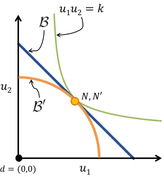
Figure 2.2: Relationship between the Nash bargaining solution and the rectangular hyperbola.
An important property of a hyperbola is that the tangency point bisects the line segment of the tangent between its asymptotes. Hence the Nash solution for a linear utility frontierBis finding the furthest hyperbola from the origin with asymptotesd1,d2 that touchesB(Fig. 2.2).
The equation of such hyperbola on an (u1, u2) plane is (u1 −d1)(u2 −d2) = k with k > 0 a
Ax4. Independence of irrelevant alternatives (IIA): If the solution for (B, d) is N, and B0 ⊆ B, N ∈ B0, then the solution of (B0, d) is alsoN.
In other words, if a linear utility frontier is reduced, in such a way that the original solutionN and disagreement point dare still included, the solution for the modified problem remains the same. For example in Fig. 2.2, the Nash solution is same for the linear bargaining setBand the reduced bargaining setB0for a common disagreement pointd. The axioms Ax1 through Ax4 are sufficient to establish that Nash solutionN always occurs where (u1−d1)(u2−d2),(u1, u2)∈ Bd,
is a maximum. However, Nash’s axiom Ax4 has been extensively discussed and criticized because it represents a player’s own loss or gain, but does not present any information about the gain or loss of the other player. Fig. 2.3 depicts the controversy reflected by Nash’s axiom Ax4: the Nash solution for the bargaining games (B, d) and (B0, d) is the same, specifically, Player 2 does not consider how much Player 1 gives up.
2.2.2 Raiffa Solution
1
1 2
′
2
1, 2
0,0
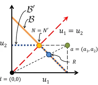
Figure 2.3: An example where Nash bargaining solution is controversial, and where Raiffa’s solution is more acceptable.
Raiffa addressed the problem with Nash’s axiom Ax4,IIA, by replacing it with the following axiom:
Ax4a. Monotonicity (Mon): If B0 ⊆ B, max{u1|(u1, u2) ∈ Bd} = max{u1|(u1, u2) ∈ B0d} and
max{u2|(u1, u2)∈ B0d} ≤max{u2|(u1, u2)∈ Bd}, thenN20 ≤N2 whereN = (N1, N2) and
frontier B, where a = (a1, a2) = (max{u1|(u1, u2) ∈ Bd},max{u2|(u1, u2) ∈ Bd}) is called the
utopia point [33]. This implies that R = (u1, u2) ∈ Bd is the solution point that maintains
the ratios of maximal gains: u2−d2 u1−d1 =
a2−d2
a1−d1. In Fig. 2.2, R is the Raiffa solution for the game
(B0, d). For a game with a linear frontier with disagreement pointd= (0,0) and utopia point a= (1,1), it is easy to validate that the Nash and Raiffa solution coincide. Since every game can be normalized by a unique affine transformation of the utilities so that the disagreement point and utopia point become d = (0,0) and a = (1,1) respectively, we conclude that Nash and Raiffa solutions coincide for any game (B, d) that has a linear utility frontier.
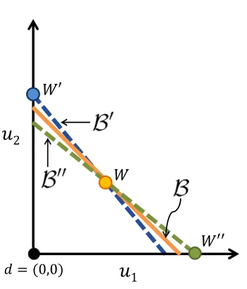
2.2.3 Utilitarian Solution
1 2
′
′′
0,0
Figure 2.4: Utilitarian solution for linear bargaining sets with slope −1 +, 1, and, −1− respectively.
The utilitarian rule by Thomson [31] chooses the pointW = (w1, w2)∈ Bdthat maximizes
the sum of the utility increments, w1 +w2, with the additional condition that the individual
utilities shall be as nearly equal as possible whenever their sum is maximum at more than one point. Thomson provided the corresponding axiomatic solution by weaking Nash’s axiom Ax3, Inv, with the following axiom, while retaining the Nash’s other three axioms namelyPO, Sym, IIA:
assumption thatai= 1, i= 1,2.
Geometrically, this solution is the tangent point of the Pareto frontier of the game (B, d) and the straight line through points (k,0) and (0, k), k > 0. However, Utilitarian rule presents a drawback when the utility frontier is linear: when the slope of the linear utility frontier is varied from −1−to−1 +, is an arbitrarily small positive quantity, the solution point shift from one axis intercept to the other, pausing at the midpoint of the linear frontier when the slope is exactly −1. For example, note in Fig. 2.4 the Utilitarian solutions, W, W0 and W00, when the slope of the linear frontier changes from −1− to −1 +, where is an arbitrarily small positive quantity. Hence the Utilitarian solution may leave one of the player with a zero utility increment, thus gaining that player’s cooperation in the game is difficult.
2.2.4 Egalitarian solution
′
1
1 2
,
2
0,0
′
Figure 2.5: Comparing Egalitarian solution and Nash solution for linear bargaining sets.
The Egalitarian solution [30,33] attempts to grant equal gains to both parties (i.e.,u1−d1=
u2−d2) by replacing Nash’s axiom Ax3 with the following axiom:
V = (V1, V2) :B−→V R2 is a transformation such that for all ( ˆu1,uˆ2)∈ B and ( ˇu1,uˇ2)∈ B:
(i) Vi( ˆu1,uˆ2)≥Vi( ˇu1,uˇ2) if and only if ˆui ≥uˇi,i∈ {1,2}, and;
(ii) V1( ˆu1,uˆ2)−V1(d1, d2)≥V2( ˇu1,uˇ2)−V2(d1, d2) if and only if ˆui−di≥uˇi−di.
This property states that if a game (B0, d0) is derived from (B, d) via a transformation V (of feasible utility vectors) which:
(i) preserves each player’s ordinal preferences and,
(ii) preserves information about which player makes larger gains at any given utility, then the same transformation applied to the final agreement of the game (B, d) should yield the final agreement of the game (B0, d0).
That is, the property states that the solution should depend only on the ordinal preferences of the players, and on the ordinal comparision of the utilities to the players at any given agreement, and not on any other features of the utilities. The Egalitarian solution satisfies axioms 1, 2, 3b and 4 and selects the outcome E = (u1, u2), where (u1, u2) is the Pareto optimal point
in B such that min{u1−d1, u2 −d2} > min{x1 −d1, x2 −d2} for all Pareto optimal points
(x1, x2) inB distinct from (u1, u2). The solution E picks the Pareto optimal point in B which
maximizes the minimum gains available to the players, as shown in Fig. 2.5. The letterE was chosen to reflect the fact that this solution selects the outcome which gives both players equal gains, whenever there exists a Pareto optimal outcome with this property. In any event, the solution E always selects the Pareto optimal point which comes closest to giving the players equal gains. The equal gains solutionE can thus be thought of as differing from Nash’s solution only in the kind of information which is assumed to determine the outcome of bargaining. Axiom Ax3 permits Nash’s solution to be sensitive to the intensity of each players’ preferences for the various potential outcomes, but requires it to be insensitive to any comparison between players (see Fig. 2.3). Axiom Ax3b, on the other hand, permits the equal gains solution E to be sensitive to comparisons of the utilities the players get at any given outcome, and to be sensitive to each players’ ordinal preferences over different outcomes, but prevents it from being sensitive to the intensity of their preferences over different outcomes.
(u1−d1)δ(u2−d2)1−δ, with weights δ and 1−δ. Thus the only role of symmetry in Nash’s
solution is to setδ= 1−δ= 0.5, which causes the solution to weight equally the gains of both players. Hence, dropping the property of symmetry in axiom Ax2 permits the Nash solution to reflect differential bargaining ability between players. Without stating the axioms, we only state the equilibrium condition for the other bargaining solutions under differential bargaining ability between players: the weighted Raiffa solution is the maximal point which maintains the ratio u2−d2
u1−d1 = δ 1−δ × a2
−d2
a1−d1, the weighted egalitarian solution (also known as the proportional
bargaining solution) is the maximal point at which the utility gains are proportional to the weights, u2−d2
u1−d1 = δ
1−δ (the solution is the point of intersection of the Pareto boundary with the
ray through points (d1, d2) and (δ,1−δ)), and the weighted Utilitarian solution is the maximal
point where weighted sum of utilities,δu1+ (1−δ)u2, is a maximum.
Chapter 3
Optimal Resource Allocation in
IEEE 802.11 Based Wireless Local
Area Networks
In this chapter, we propose a channel access method for the multi-rate enterprise Wireless Local Area Network (WLAN) (as shown in Fig. 3.1) that will maintain weighted time fairness or weighted throughput fairness among the users in a WLAN cell. All the WLAN nodes (primary users, secondary users and the APs) use the proposed channel access method to gain access to the medium for their data transmission.
User AP
INTERNET
ETHERNET
CONTROLLER
2.4 GHz Ch1
2.4 GHz Ch6 2.4 GHz Ch11
Table 3.1: Notations used throughout this chapter.
Notation Description
pi The channel access probability of user iinCj.
CWi The contention window of useriin Cj.
Pidle The probability that a slot is idle.
Pc The probability of collision in a slot time.
Pti The successful transmission probability of user iinCj.
Tc The average collision duration of users in a WLAN cell.
Tti The transmission duration of useri.
Tslot The duration of an empty slot.
sd The average packet payload size in bits.
n The number of users in the WLAN cellCj.
xi The throughput of user i.
X The aggregate throughput of all users.
We begin the discussion with the assumption that the WLAN cell under study does not suffer from inter-cell contention with other WLAN cells, i.e., we consider the case
Φj = 1, ∀j∈ A, (3.1)
whereAis the set of all APs in the network and Φj is the fraction of the time the WLAN cell of
AP j has access to the medium. We later extend our results to the case 0<Φj ≤1 where the
WLAN cells suffer from inter-cell contention. The proposed WLAN model adopts a medium access mechanism very closely related to 802.11 DCF access mechanism, but which, instead of the binary exponentially backoff mechanism in DCF uses a fixed contention window for every access attempt. This approach improvesshort-term fairness1, and has been adopted in several works on WLAN optimization [17, 20–22, 34]. We assume a saturated WLAN cell with nusers where each competing user always has packets to transmit, and each user uses the same packet payload size,sd(in our numerical results we usesd= 12000 bits). We consider an ideal channel
where packet losses are only due to packet collisions. Table 3.1 lists the notations used in this chapter.
We consider a single WLAN cell in the enterprise network, e.g., WLAN cell of AP j, j ∈
A, and denote its associated users with the set Cj. Consider the event where user i ∈ Cj is
attempting to transmit a packet of sizesdin a given time slot. The attempt probability can be 1
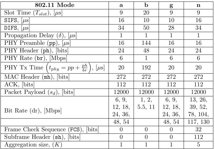
Table 3.2: Parameters used to obtain numerical results.
802.11 Mode a b g n
Slot Time (Tslot), [µs] 9 20 9 9
SIFS, [µs] 16 10 10 16
DIFS, [µs] 34 50 28 34
Propagation Delay (δ), [µs] 1 1 1 1
PHY Preamble (pp), [µs] 16 144 16 16
PHY Header (ph), [bits] 24 48 24 24
PHY Rate (br), [Mbps] 6 1 6 6
PHY Tx Timetphy =pp+phbr
, [µs] 20 192 20 20
MAC Header (mh), [bits] 272 272 272 272
ACK, [bits] 112 112 112 112
Packet Payload (sd), [bits] 12000 12000 12000 12000
Bit Rate (dr), [Mbps]
6, 9, 1, 2, 6, 9, 13, 26, 12, 18, 5.5, 11 12, 18, 39, 52,
24, 36, 24, 36, 78, 104,
48, 54 48, 54 117, 130
Frame Check Sequence (FCS), [bits] 0 0 0 32
Subframe Header (sh), [bits] 0 0 0 112
Aggregation size, (K) 1 1 1 5
calculated as in [20] when the exponential binary backoff is disabled:
pi=
2 CWi+ 1
, i∈ {1, . . . , n}. (3.2)
The expression for Pti, Pidle, Pc can be calculated as [20]:
Pti =pi
n
Y
k6=i,k=1
(1−pk), i∈ {1, . . . , n}, (3.3)
Pidle= n
Y
i=1
(1−pi), (3.4)
Pc= 1−Pidle− n
X
i=1
Pti. (3.5)
The per user throughput [20]xi for user iis:
xi =
Ptisd Pn
k=1PtkTtk+PcTc+PidleTslot
where
Tti =tphy+
mh+K(sh+sd)
dri
+FCS dri
+δ+SIFS+tphy+
ACK
dri
+δ+DIFS, (3.7) Tc=tphy+ [mh+K(sh+sd)]E
1 dri +FCS dri
+δ+DIFS, (3.8)
with the parameters defined in Table 3.2. The aggregate throughput of the WLAN cell, X, is:
X =
n
X
i=1
xi=
Pn
i=1Ptisd Pn
i=1PtiTti +PcTc+PidleTslot
. (3.9)
0 1.5 3 4.5
1.5 3 4.5 6 7.5 x
1 (Mbps)
x 2
(Mbps)
Rate region boundary
(a)
0 1.5 3 4.5
1.5 3 4.5 6 7.5 x
1 : x2 = 1 : 1 x
1 : x2 = 1 : 2
x
1 : x2 = 2 : 1 x
1 : x2 = 1 : 8
x
1 : x2 = 1 : 4
x
1 : x2 = 6 : 1
x
1 (Mbps)
x 2
(Mbps)
Rate region boundary
(b)
Figure 3.2: The rate region of an 802.11b multi-rate WLAN with two nodes where the bit rate of node 1 is 5.5 Mbps and node 2 is 11 Mbps. Each point in the rate region represents the throughput allocation for a certain chosen channel access probability by the users.
3.1
WLAN Model for Time Fairness
The weighted time fairness constraint require the contending users to share their successful channel occupancy timein proportion to their weights:
PtiTti
PtkTtk = wi
wk
, i, k∈ {1, . . . , n}. (3.10)
The rate region of a multi-rate IEEE 802.11 WLAN is the set of achievable throughputs of the users as their channel access probability ranges over the domain [0,1]. Fig. 3.2-(a) depicts the rate region of a IEEE 802.11b multi-rate WLAN with two users, with user 1 using 5.5 Mbps and user 2 using 11 Mbps. In contrast to TDMA based systems, 100% utilization of the wireless medium is not feasible in a WLAN cell due to the random backoff of DCF. Hence, a single user in a WLAN cell cannot achieve a throughput equal to its link bit rate, as observed in Fig. 3.2-(a). Moreover, there is always a strictly positive packet collision probability when multiple users contend for the channel access, and hence the time-sharing argument2 [35, 36] does not apply for random access networks. Therefore, the rate region of an 802.11 WLAN is non-convex (Fig. 3.2-(a)) [36–39]. Although the rate region is non-convex, [36–39] prove that the complement of the rate region in the positive orthant is strictly convex.
From (3.6) and (3.10), we have:
xi
xk
= Pti
Ptk =
wti Tti wtk Ttk
, i, k∈ {1, . . . , n}. (3.11)
From (3.11), all the throughput allocations in the rate region that lie on the ray passing through [0, . . . ,0] andhw1
Tt1, . . . , wn
Ttn i
have the same user weights [w1, . . . , wn] but different throughputs
[x1, . . . , xn]. Among all the throughput allocations on this ray, the throughput allocation with
the maximum aggregate is on the rate region boundary, as shown in Fig. 3.2-(b). Hence, for any user weights [w1, . . . , wn], the optimal throughput allocation is on the rate region boundary.
Therefore, we calculate the channel access probability for the users that will satisfy the weighted time fairness constraint in (3.10) and also maximize the aggregate network throughput X in (3.9).
If we letqi= 1−pipi in the condition for weighted time fairness in (3.10), we have:
Pti
Ptk
= pi(1−pk) pk(1−pi)
= qi qk = wi Tti wk Ttk . (3.12) 2
After calculations, it can be shown that maximizing the network throughputX in (3.9) for the condition in (3.12) is equivalent to minimizing the following cost function:
C(qi) =
Qn
k=1(1 +qk)
qi
Tc+
1 qi
(Tslot−Tc). (3.13)
The first derivative (with respect toqi) of the cost function in (3.13) is
dC(qi)
dqi
= qi Pn
k=1 dqk
dqi Qn
l6=k(1 +ql)−Qnk=1(1 +qk)
qi2 Tc−
1
qi2(Tslot−Tc), (3.14) =
Pn
k=1qkQnl6=k(1 +ql)−Qnk=1(1 +qk)
qi2 Tc−
1
qi2(Tslot−Tc), (3.15)
= −
1−Pn
k=1 1+qkqk
Qn
k=1(1 +qk)
qi2 Tc− 1
qi2(Tslot−Tc). (3.16) Setting the first derivative of the cost functionC(qi) in (3.16) to zero:
1−
n
X
k=1
wkqi Ttk
Ttiwi+wkqi
n Y k=1
1 +wkTti
wiTtk
qi
= 1−Tslot Tc
. (3.17)
Solving qi in (3.17) for each node i∈ {1, . . . , n} results in the optimal contention window size
for the nodes3 that will maintain their time shares in the ratios [w1, . . . , wn] while
simultane-ously maximizing the aggregate network throughput. The work in [17] derives the equivalent polynomial expression for (3.17) in terms of the contention window, CWi, when all user have
the same weights (i.e., w1 = . . . = wn = 1). It is shown in [17] that the optimal contention
window of user i,CWi, is obtained by solving the following polynomial:
λ2
(CWi−1)2
+ 2λ3 (CWi−1)3
+· · ·+ (n−1)λn (CWi−1)n
= Tslot Tc
, (3.18)
wherehj = 2TTti
tj is used to compute:
λk=
X
l1<l2<···<lk 1≤l1,l2,···,lk≤n
hl1hl2 · · ·hlk, k= 1,2,· · ·, n. (3.19)
Uniqueness of CWi is shown in [17]. The work in [17] can be easily extended to support the
weighted user case, where the optimal contention window of the user is obtained by the same polynomial in (3.18) with λk, k∈ {1, .., n}, defined in (3.19) but with a new definition for hj
given by:
hj =
2wjTti
wiTtj
. (3.20)
Rewriting the first derivative of the cost functionC(qi) in (3.16) in terms of the channel access
probability of the nodes [p1, . . . , pn] and setting the expression to zero:
1−
n
X
i=1
pi =
1−Tslot Tc
n Y
i=1
(1−pi). (3.21)
The expression in (3.21) is the condition for the throughput allocation to lie on the rate region boundary. Solving (3.17) involves finding roots for a polynomial of order n, where n is the number of users in the WLAN cell. A medium access control algorithm that requires solving a polynomial of higher order is clearly infeasible in real time. To counter this problem, we use a simple yet accurate approximation, and show that the approximation leads to a simplified equivalent solution that calculates the same channel access probability in (3.10) and (3.21) but at a greatly reduced computation cost. Since the access probability of any of the users pi1,
Table 3.3: ParametersTslot,Tc,η andζfor 802.11 a/b/g/n.
a b g n
Tslot[µs] 9 20 9 9
Tc [µs] 861.06 5.7×10³ 855.06 1.6×10³
η 0.9895 0.9965 0.9895 0.9943
ζ 0.1380 0.0816 0.1385 0.1035
the following approximation holds: 1−pi
1−pk ≈
1, i, k ∈ {1, . . . , n}. (A1)
Using (A1) in (3.10),
pk=pi
wkTti
wiTtk
, i, k ∈ {1, . . . , n}. (3.22)
and when n−→ ∞,
n
Y
k=1
(1−pk)−→e− Pn
k=1pk =e−pi
Pn k=1wkTtiwiTtk
where
τi =
Tti
wi n
X
k=1
wk
Ttk
, i∈ {1, . . . , n}. (3.24)
The transmission durationTti depends on the link bit rate of useri, the parameters of MAC and PHY layers (802.11 a/b/g) and the average data packet sizesd. Consequently, the transmission
duration for all supported bit rates of the chosen 802.11 variant can be precomputed and stored in a lookup table. Therefore, calculatingτi only requires knowledge of the user weights and the
link bit rates of the users in the WLAN cell. Using (3.23) and (3.24) in (3.21), we have: 1−τipi =ηe−τipi, i∈ {1, . . . , n}, (3.25)
where η = 1− Tslot
Tc can be calculated for a given variant of 802.11 from the parameters of the MAC and PHY layers (Table 3.3). Since (3.25) is a transcendental equation involving exponential, its closed form solution is given in terms of the Lambert W function (W) [40] (also see Appendix A):
pi =
W −ηe + 1 τi
, i∈ {1, . . . , n}. (3.26)
Since −1/e <−η/e <0 and W(−η/e)>−1 because the access probabilitypi >0 and τi >0,
we have:
pi=
W0 −ηe
+ 1 τi
, i∈ {1, . . . , n}, (3.27)
whereW0(·) is the principal branch ofW and is a single-valued function. The value of
ζ =W0
−ηe+ 1, (3.28)
is a fixed constant for a given 802.11 variant since it only takesη and eas its arguments (Ta-ble 3.3). Hence the channel access probability of useriis:
pi =
ζ τi
, i∈ {1, . . . , n}, (3.29)
whereτi is defined in (3.24), is unique and its calculation only requires performing an addition
Also, from (3.23), (3.27):
n
X
i=1
pi =τipi=ζ. (3.30)
Furthermore using (3.30) in (3.3), (3.4), (3.5), we obtain the following approximations which we will use later in Chapter 4 for deriving the closed-form expression for the bargaining set in the CCRN framework in chapters 4 and 5:
Pidle≈e−ζ, (3.31)
n
X
i=1
Pti ≈ζe
−ζ, (3.32)
Pc≈1−ζe−ζ−e−ζ. (3.33)
3.2
WLAN Model for Throughput Fairness
Under weighted throughput fairness constraint, the contending users share their achievable throughputs in proportion to their weights:
xi
xk
= Pti Ptk
= pi(1−pk) pk(1−pi)
= wi wk
, i, k∈ {1, . . . , n}. (3.34)
Weighted time fairness and weighted throughput fairness constraints are equivalent upon rescal-ing the user weights with their transmission time:
Pti
Ptk = wi
wk ⇐⇒
PtiTti
PtkTtk
= wiTti
wkTtk
, i, k∈ {1, . . . , n}. (3.35)
Therefore, we can view the weighted throughput fairness constraint as a special case of the weighted time fairness constraint. Replacing wi with wiTti in (3.17) (equivalently, in (3.20)) results in the polynomial expression:
1−
n
X
j=1
wjqi
wi+wjqi
n Y j=1 1 +wj
wi
qi
= 1−Tslot
Tc
, (3.36)
throughput. Similarly, for the proposed WLAN model in (3.29), the expression forτi becomes:
τi =
1 wi
n
X
k=1
wk, i∈ {1, . . . , n}. (3.37)
3.3
Performance Evaluation
3.3.1 Performance Evaluation with Time Fairness Constraints
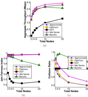
In Fig. 3.3, we compare the performance of our proposed approximate WLAN model with other well-known WLAN models for the case where all the users in the WLAN cell have equal weights, i.e., there is no service differentiation among the users. The WLAN models used in the performance evaluation are:
(i) theoptimalchannel access probability of users obtained by solving the polynomial in (3.17). (ii) the default 802.11 DCFbackoff algorithm;
(iii) the proportional fair throughput allocation algorithm proposed by Banchs et al in [34]; (iv) the idle sense algorithm in [21].
We have developed a discrete-event simulator that implements the standard 802.11 DCF (no RTS/CTS) for each independently transmitting station. The support for the remaining access methods under consideration are built on this simulator. The simulator uses MAC and PHY parameters of IEEE 802.11b standard for a packet size of 1500 bytes and is run for a simulation time of 200 seconds for each experiment. We consider a 802.11b WLAN with one slow node with link bit rate of 1 Mbps and all the remaining users use a link bit rate of 11 Mbps. We determine:
(i) the aggregate network throughput;
(ii) the short-term fairness of the channel occupancy time using the sliding window method4 in [41, 42] to compute the average Jain fairness index [43].
2 3 4 5 10 20 1.5 2.5 3.5 4.5 5.5 6.5 Total Nodes
Aggregate Throughput (Mbps)
Approximate Optimum DCF Idle Sense Banchs (a)
2 3 4 5 10 20
0.4 0.5 0.6 0.7 0.8 0.9 1 Total Nodes
Jain Fairness Index
Approximate Optimum DCF Idle Sense Banchs (b)
3 4 5 10 20 0.2 0.6 1 1.4 1.8 Total Nodes Collision Ratio Approximate Optimum DCF Idle Sense Banchs (c)
Figure 3.3: Performance comparison of the five MAC algorithms under time fairness: (a) ag-gregate throughput of the WLAN, (b) short-fairness of the channel occupancy time, and, (c) collision overhead.
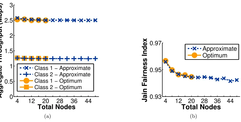
In Fig. 3.4, we evaluate the performance of the proposed approximate algorithm when the 802.11b WLAN has two traffic classes, class1 and class2, with the desired channel occupancy
time ratios set tow1 = 1 and w2 = 0.5 respectively. Only one class is active for a user: half of
the users sendclass1traffic, while the other half sends class2 traffic; and within each class, half
4 12 20 28 36 44 0
0.5 1 1.5 2 2.5 3
Total Nodes
Aggregate Throughput (Mbps)
Class 1 − Approximate Class 2 − Approximate Class 1 − Optimum Class 2 − Optimum
(a)
4 12 20 28 36 44
0.93 0.95 0.97
Total Nodes
Jain Fairness Index
Approximate Optimum
(b)
Figure 3.4: Proportional time allocation in a 802.11b WLAN with two traffic classes: (a) Ag-gregate throughput per classvs. number of nodes under; (b) short-term fairness of the channel occupancy.
3.3.2 Performance Evaluation with Throughput Fairness Constraints
We use the 802.11e EDCA model in idle sense [22] and compare its performance with the proposed WLAN model. We consider the same WLAN set in the simulation experiment in Sec-tion 3.3.1. We set the desired throughput ratios tow1 = 1 andw2= 0.5 (similar to the scenario
in Figure 3 of [22]). To obtain this allocation, we set the following parameters of 802.11e in our simulator (from [22]):CW1∈[16,48] for class 1 andCW2 ∈[31,93] for class 2. In Fig. 3.5-(a),
we calculate the aggregate network throughput for each traffic class and in Fig. 3.5-(b) we show the short-term fairness of channel access opportunities. The results in Fig. 3.5 show that the proposed WLAN model agrees with the optimal performance and that the model achieves the desired throughput ratio 1:0.5. The results also show that the aggregate throughput of the classes does not depend on the number of nodes when using our models while with 802.11e the aggregate throughput decreases.
3.4
Support for Downlink Traffic
4 12 20 28 36 44 0.1 0.3 0.5 0.7 0.9 1.1 Total Nodes
Aggregate Throughput (Mbps)
Class 1 − Approximate Class 2 − Approximate Class 1 − Optimum Class 2 − Optimum Class 1 − 802.11e Class 2 − 802.11e
(a)
4 12 20 28 36 44
0.95 1
Total Nodes
Jain Fairness Index
Approximate Optimum 802.11e
(b)
Figure 3.5: Proportional throughput allocation in a 802.11b WLAN with two traffic classes: (a) Aggregate throughput per class vs. number of nodes under; (b) short-term fairness of the channel occupancy.
traffic. We consider only the time fairness case in this section. Support for downlink traffic for the throughput fairness case is easily obtained by replacing the user weights wi with wiTti in the final results for the time fairness case (by virtue of the result in (3.35)). Let the weight of user ion the downlink is ˇwi =wd×wi, wherewd is the weight for downlink traffic relative to
uplink traffic. We setwd= 3 in our simulation experiments. Letqi denote the access probability
the AP assigns to userifor its downlink traffic. We refer to the AP of the WLAN cell as user n+ 1. The access probability of the AP is:
pn+1 = n
X
i=1
qi. (3.38)
The condition for proportional time allocation is: PtiTti
wi
= PtkTtk
wk
= QtiT 0
ti ˇ wi
= QtkT 0
tk ˇ wk
, ∀ i, k∈ {1, . . . , n}, (3.39)
where Tti and T 0
ti are the transmission time of user i on its uplink and downlink respectively;
Pti is the successful transmission probability for user iand follows the definition in (3.3); Qti is the successful transmission probability for AP to transmit a packet to user idefined as:
Qti =qi
n
Y
k=1
Using (3.39) and (3.40), we can show that the AP is a separate user with channel access probability pn+1 in (3.38), user weight:
wn+1=
X
i∈Cj ˇ wi =wd
n
X
i=1
wi, (3.41)
and transmission time:
Ttn+1 = Pn
i=1wi
Pn
i=1Tw0i ti
. (3.42)
Internally, the AP assumes the users as individual virtual stations contending for a transmission opportunity each with access probability:
vi =
qi
pn+1
= Pnwi
k=1wk ×
Ttn+1
Tt0i =
wi
T0 ti Pn
k=1Tw0k tk
. (3.43)
The optimal and approximate access probabilities for then+1 nodes (nusers and the AP) are calculated using (3.17) and (3.29) respectively.
3.5
Accounting for the Effects of Inter-Cell Contention
Thus far we assumed the WLAN cell does not suffer from inter-cell contention. However in a densely deployed enterprise WLAN, the AP suffers from high Radio Frequency (RF) interference and inter-cell channel contention from other co-channel neighboring APs. In this section, we account for the loss in the channel access opportunities due to inter-cell contention. Again, we consider only the time fairness case in this section. The support for downlink for the throughput fairness case is easily obtained by replacing the user weights wi with wiTti in the final results for the time fairness case.
Let Φj represent the fraction of channel access time the WLAN cell of AP j is entitled to
have (for receiving or sending packets) with respect to other WLAN cells that are in the AP’s collision domain. Therefore, the aggregate channel access time of the users in the WLAN cell of AP j must be proportional to Φj, while the remaining fraction of the channel access time,
1−Φj, is lost to other WLAN cells in its collision domain. The lost channel access opportunities
“big user” occupies the channel for a period equivalent to the fraction 1−Φj , i.e.,
Ptn+2Ttn+2 Pn+1
k=1PtkTtk
= Φj 1−Φj
. (3.44)
where the index n+ 2 represents the big user, index n+ 1 represents the AP j and index
{1, . . . , n} represent the users in the WLAN cell of APj. From (3.44) and (3.3), we can show that each user in the WLAN cell views the “big user” as any other contending user with user weight:
wn+2 =
1−Φj
Φj n+1
X
k=1
wk, (3.45)
and transmission time:
Ttn+2 = Pn+1
k=1wk
Pn+1
k=1 Twtkk
. (3.46)
Using (3.45) and (3.46) in the expression for τi in (3.24), we obtain:
τi =
1 Φj
Tti
wi n+1
X
k=1
wk
Ttk !
, i∈ {1, . . . , n+ 1}. (3.47)
The optimal access probabilities for the n+2 nodes (n users, the AP and the “big user”) are calculated using (3.17) with the weight, transmission time for the AP and the “big user” are given by the expressions (3.41), (3.42) and (3.45), (3.46) respectively. The approximate access probability for users and the AP are calculated using (3.29) forτi defined in (3.47).
The quantity Φj represents the level of contention in the cell of AP j’s neighborhood and
takes a value in (0,1]. For example, if two AP’s are within each other’s carrier sensing range, then Φj ≈0.5 for each WLAN cell, because the 802.11 MAC algorithm arbitrates the channel access
such that each WLAN cell will acquire the medium for approximately 50% of a reference period. Several earlier works have attempted to characterize Φj and have shown that the problem is
non-trivial due to the complex interaction of multiple contention domains in a densely deployed network. A measurement-driven model is proposed in [45], where over a measurement period of five transmission/reception events, the number of slots the AP consumes in one of the following states are calculated: transmitting or receiving; idling and; the back-off stage. The measurements are then used to estimate Φj, the fraction of the reference period, during which the AP succeeds