On Nonparametric Estimation of the Latent
Distribution for Ordinal Data
Sujit K. Ghosh
∗, Christopher Burns, Daniel Prager
†, Li Zhang,
and Glenn Hui
‡Last revised on: September 14, 2016
Abstract
Ordinal data collected in surveys often consist of numerical scores that
have a natural ordering. Observed values of ordinal variables can be thought
of as a manifestation of some underlying continuous latent variable which
is related to the observed ordinal variable through a set of threshold or
“cut-points”, which partition the latent variable into intervals
correspond-ing to the observed levels of the ordinal variable. This latent distribution
is of interest to researchers for purposes of descriptive statistics and
sta-tistical modeling. However, restrictive parametric assumptions about the
latent distribution are often not adequate. A nonparametric model based
on mixtures of scaled Beta distributions is presented and estimation is
car-ried out using a version of Anderson-Darling statistic based criteria which
is shown to be computationally efficient than likelihood based criteria. A
Monte Carlo simulation shows that proposed model and estimation method
∗Sujit Ghosh is a Professor in the Department of Statistics at North Carolina State University.
email for correspondance: [email protected]
†Christopher Burns and Daniel Prager are economists at the USDA Economic Research
Ser-vice
‡Li Zhang and Glenn Hui are graduate students at George Mason University
performs well and is robust against any underlying continuous distribution.
Several empirical examples based on ordinal data from the household
sec-tion of the Agricultural Resource Management Survey (ARMS) illustrate
the versatility and adaptivity of the method in practice.
Keywords: Anderson-Darling Statistics; Bernstein polynomials; Quadratic
1
Introduction
Ordinal data often arise in surveys of individuals or households. Examples include
questions asking respondents to state their preferences on a Likert scale (e.g.,
agree, somewhat agree, somewhat disagree, disagree) or to report their education or
income using value codes. With value-coded variables, ordinal data can represent
discrete realizations of an unmeasured continuous variable (e.g., years of education
or income in dollars). The lower and upper limits of this interval can be viewed as
cut-points in the latent continuous distribution. Observed sampled values on the
ordinal scale only provide limited information about the latent distribution, which
is partially observed through windows of adjacent intervals separated by an upper
and lower cut-point (Tamhane, Ankeman and Yang, 2002). Thus far, inference for
this latent distribution has primarily focused on parametric methods.
1.1
Latent Distribution Estimation using Parametric
Fam-ily
The Beta distribution has been proposed as a model for ordinal data on the [0,1]
interval or data transformed to this scale. A study by Tamhane, Ankeman and
Yang (2002) uses the Beta distribution as a model for the latent response because
of its finite domain and flexibility. They compare estimation methods based on
maximum likelihood by matching sample and theoretical moments, finding that
maximum likelihood estimation is typically more efficient but suffers from
con-vergence issues near the boundaries of support. Moreover, it is well known that
maximum likelihood estimates (MLE) are efficient only under the assumption that
the true underlying distribution belongs to specified parametric family. For
in-stance, when the true underlying latent variable has a log-normal distribution and
MLEs are obtained by assuming a Gamma family, the density estimate is no longer
There is vast literature on modeling ordinal data as polychotomous and binary
response data (see Agresti and Kateri 2010 or Johnson and Albert 2006 for a
review). Statistical inference is based on a continuous latent response distribution
from a known parametric family. The classical approach fits a categorical response
regression model using maximum likelihood. Examples include the logit, probit,
and ordered logit or probit models, which assume a logistic or normal distribution
for the latent variable (Winship and Mare 1984). McCullagh (1980) examines the
proportional odds and proportional hazard models. Both assume a parametric
distribution for the latent response. Confirmatory factor analysis uses normality
assumptions to examine hypothesized relations among ordinal variables (Flora and
Curran 2004).
Bayesian methods for estimating a parametric latent density have also been
explored. Albert and Chib (1993) use Gibbs sampling combined with data
aug-mentation to sample from the posterior distribution of a latent density. They
develop a generalized approach that can be used to fit multinomial, hierarchical,
and ordered probit regression models.
However, parametric assumptions about the latent distribution may not be
appropriate in some cases. In these circumstances a more flexible class of statistical
models are needed, which can include mixture distributions, as well as kernel and
spline-based density estimation methods.
1.2
Nonparametric Methods
Nonparametric density estimation is a popular alternative when the underlying
true distribution can not be safely assumed to arise from a known parametric family
of distributions. The most popular nonparametric method for density estimation
is the kernel method (Parzen 1962). This method uses the weighted average of the
chosen kernel functions centered at the observed values and a bandwidth parameter
While numerous parametric models exist for ordinal data, there has been little
research into nonparametric methods. Kottas, Muller, and Quintana (2005)
pro-pose a nonparametric method for modeling multivariate ordinal data based using
Bayesian methods to estimate a variation of a multivariate probit model. Shah
and Maden (2004) demonstrate a method for nonparametric analysis of ordinal
data in a designed factorial experiment. Sequence of Bernstein polynomials, which
can be viewed as mixtures of (scaled) Beta densities, represent another
nonpara-metric class of densities that has been shown to provide consistent estimate of
unknown continuous density and has asymptotic properties similar to kernel and
spline based density estimates.
1.3
Density Estimation using Sequence of Bernstein
Poly-nomials
Bernstein polynomials are a polynomial approximation approach to density
esti-mation that fits a flexible class of a mixture of (scaled) Beta densities. Vitale
(1975) was the first to propose the use of Bernstein polynomials for density
es-timation. Babu, Canty and Chaubey (2002) explore the asymptotic properties
of Bernstein polynomial and show how they can be adapted for smooth
estima-tion of a distribuestima-tion funcestima-tion supported on a bounded interval. They also show
that Bernstein polynomials may be preferable to the kernel-density estimator
un-der certain circumstances. Leblanc (2012a) explores higher orun-der expansion for
the asymptotic (integrated) mean-squared error of Bernstein estimators and finds
they outperform empirical distribution functions. Further work by Leblanc (2012b)
studies the properties of Bernstein polynomials with bounded support and finds
the estimator to have less bias and variance in the boundary regions.
Recent developments have explored both the speed and convergence of the
Bernstein approximation and advanced the use of Bernstein polynomials with
non-parametric density estimation. Ghosal (2001) and Petrone and Wasserman (2002)
show that under mild assumptions a Bernstein polynomial prior will provide a
con-sistent posterior density. Leblanc (2010) shows how a bias reduction method can
lead to a Bernstein polynomial estimator that converges at a faster rate. Mant´e
(2015) shows how to use the eigenstructure of the Bernstein operator to improve
the convergence of the Bernstein polynomial method.
A recent study by Turnbull and Ghosh (2014) uses Bernstein polynomials to
approximate an unknown continuous unimodal density. They show that estimation
of the mixing weights can be accomplished by minimizing a version of
Anderson-Darling (AD) statistic (Anderson and Anderson-Darling 1954), leading to a weighted least
squares criteria subject to a set of linear inequality constraints. Thus, the
esti-mates can be computed efficiently using quadratic programming methods. This is
advantageous compared to a maximum likelihood method which requires nonlinear
optimization techniques.
While there is a large literature on Bernstein polynomials, we are not aware of
any studies that use this method to estimate the latent density for ordinal data.
This paper adds to the current literature by using cut-point methods to estimate
the latent density of ordinal data using Bernstein polynomials. We also extend the
unimodal density estimator developed in Turnbull and Ghosh (2014) to consider
multimodal latent densities.
This paper presents a method for estimating a the latent density of ordinal
data using both parametric and nonparametric methods. Section 2 presents the
general modeling framework and associated estimation methods based on
maxi-mum likelihood and the AD method. In Section 3, we provide several empirical
scenarios based on simulated data sets to exhibit the performance of the proposed
AD method and compare them with maximum likelihood-based methods. In
Sec-tion 4, we illustrate the methodologies on several ordinal variables obtained from
for future research.
2
Methodology
Consider a sample of n ordinal observations X1, X2, . . . , Xn that are an
indepen-dently and identically distributed (i.i.d) sequence of an ordinal random variableX.
Assume that the random variableX takes on finitely many value codes 1,2, . . . , m
with probabilities p1, p2, . . . , pm, respectively; in other words, pk = Pr[X = k] for
k = 1,2, . . . , m. Using the well-accepted notion that ordinal variables are simply a
manifestation of some underlying continuous variable, we propose a method that
models the observed ordinal variable against this latent continuous variable. We
take a completely flexible approach by employing a linear combination of basis
functions to model the latent distribution.
The latent variable is of course unobserved, but is related to the observed
ordinal variable through a set of threshold or “cut-points”, which partition the
latent variable into intervals corresponding to the observed levels of the ordinal
variable. More formally, we assume that the observed realization of the ordinal
variable X is related to a latent continuous variable U by the following: X =
∑m
j=1I(U > cj−1), where U ∈R and −∞ ≤c0 < c1 < c2 <· · ·< cm−1 < cm ≤ ∞,
are known ordered cut-points. If F(u) = Pr[U ≤ u] denotes the distribution
function, then it follows that pk =F(ck)−F(ck−1) because X = k if and only if
ck−1 < U ≤ck. We assume throughout thatF(c0) = 0 = 1−F(cm). The goal here
is to estimate the unknown distribution function F(·) based on ni.i.d. realizations
of the ordinal random variable X. The nonparametric log-likelihood function is
given by
L(F) = m ∑
k=1
fklog[F(ck)−F(ck−1)] where fk =
n ∑
i=1
ˆ
F such that ˆF(ck) =
∑k
j=1fj/n. Thus, it is evident that we cannot
(nonparanter-ically) estimate the distribution function F except at the cut-points. So, in order
to estimate F we need to make further assumptions about F.
To begin with, we assume a parametric form for F given by F(x) = F0(x,θ)
where F0(·) is a known functional form with unknown parameter vector θ, then
the log-likelihood function is given by
L(θ) = m ∑
k=1
fklog[F0(ck,θ)−F(ck−1,θ)], for θ ∈Θ, (2)
which can in principle be maximized to obtain the maximum likelihood
esti-mate (MLE) ˆθ = argmaxθL(θ) and standard asymptotic inference can be made
about the estimated distribution function ˆF(x) = F0(x,θˆ) or the density function
ˆ
f(x) = f0(x,θˆ). For our empirical analysis, we explored a few popular classes
of parametric functions, such as the normal, laplace (or double exponential) and
gamma distributions, and obtained the MLE based on maximizing (2) by using
popular numerical optimization methods (e.g., the mle function in the R
pack-age stats4). Although the parametric likelihood-based method works reasonably
well for many practical scenarios and is known to provide (asymptotically) most
efficient estimates when the parametric form is assumed to be correct, we have
no universal method to choose the functional form F0(·). Hence, we develop a
more flexible functional form which can adapt to almost arbitrary shape of the
(unknown) distribution or density function of the latent variable U.
Assume that both c0 and cm are finite. Consider the following mixture of
(scaled) Beta distributions:
F0(x,θ) = N ∑
l=1
θlB (
x−c0
cm−c0
, l, N −l+ 1 )
where θl ≥0∀l and
N ∑
l=1
θl = 1.
(3)
In above B(·, l, N −l+ 1) denotes the distribution function of aBeta(l, N−l+ 1)
random variable, which can be evaluated using standard numerical methods (e.g.,
a legitimate distribution function for any θ ∈ SN ≡ {(θ1, . . . , θN) ∈ [0,1]N : ∑N
l=1θl = 1}andN ∈ {2,3, . . .}. It follows that the corresponding density function is given by
f0(x,θ) = N ∑
l=1
θlb (
x−c0
cm−c0
, l, N −l+ 1 )
1
cm−c0
for θ ∈SN, (4)
where b(u, l, N−l+ 1) =N(Nl−−11)ul−1(1−u)N−lI(u∈[0,1]) denotes the density of
the Beta(l, N−l+ 1) random variable, which can be efficiently evaluated even for
large N using standard software packages (e.g., R function dbeta can be used).
Assuming thatc0andcmare finite valued, one of the most useful and well known
results is that if U has a continuous density f(x) supported on [c0, cm], then by
choosing ˜θl =f(c0+(l−1)(cm−c0)/(N−1)), one can show by Bernstein-Weierstrass
Theorem (Lorentz, 1986) that f0(x,θ˜) converges uniformly on [c0, cm] to f(x) as
N → ∞. In other words, (4) provides a very flexible framework to estimate the
unknown continuous density of the latent variable U for a reasonably large value
of N. The appropriate value of N can be chosen based on the observed frequency
counts. In particular, for continuous data, Babu et al. (2002) recommends selecting
N ∈ {2,3, . . .[n/logn]} based on asymptotic considerations.
We can plug in the flexible functional form of (3) into the likelihood (2) to
estimate θ ∈SN for a given N; however, we find such a methodology is not
com-putationally efficient. Instead, following the recent work by Turnbull and Ghosh
(2014), we use an Anderson and Darling (AD) statistic-based criteria to estimate
θ ∈ SN using computationally stable and efficient quadratic programming (QP)
method (e.g., we use the functionsolve.QPavailable in the R packagequadprog).
In particular, we solve the following QP:
ˆ
θ = arg min
θ∈SN
m ∑
k=1
( ˆF(ck)−F0(ck,θ))2
( ˆF(ck) +ϵ)(1−Fˆ(ck) +ϵ)
, (5)
where ϵ = 3/8n and ˆF denotes empirical distribution estimate of F obtained by
F0(x,θ) as defined in (3) is a linear function of θ and hence the AD objective
function in (5) is a positive definite quadratic function of θ which has a unique
minimum in the compact set SN. The details of computing the estimate in (5) by
using the QP method are similar to those available in the Appendix of the Turnbull
and Ghosh (2014) and hence omitted here. Once ˆθ is obtained by solving the
optimization problem in (5), we can obtain the distribution and density estimate
of the latent variable by plugging in the estimate in the functional form given by
(3) or (4) for subsequent statistical inference.
2.1
Criteria to select
N
Although the methodology described above works for any given value ofN, in
prac-tice we need to select N based on the observed frequency counts fk’s as described
in (1).
The criteria for selecting the number of weightsN (i.e., the dimension of θ) is
an important issue from both theoretical and computational aspects. In theory,
selecting too many weights can lead to losses in efficiency and over-fitting of the
observed data whereas selecting too few weights can lead to a biased estimate of the
underlying density. Thus, the well-known balance between the bias and variance
is required here. Moreover, from a computational perspective, numerical stability
(e.g., positive definiteness of the matrix involved within the QP) of optimization
method in (5) is required in practice when N is chosen close to m. When N is
chosen to be larger than m, we use the Moore-Penrose generalized inverse of the
matrix to solve the optimization problem. Details of the implementation of our
algorithm and accompanying R code are available upon request from the authors.
Several studies have proposed methods for selection of the optimal number of
weights based on observations from a continuous variable. Babu et al. (2002)
show that estimated density (by mixtures of Betas) will converge uniformly to
and Ghosh (2014) investigate several methods for selecting the optimal number of
weights based on observed data. They propose a new criteria called the Condition
Number (CN), and examine the well-known Akaike Information Criterion (AIC)
and Bayesian Information Criterion (BIC) as well. The CN uses information about
the absolute value of the ratio of maximum and minimum eigenvalues to select the
optimal number of weights. They find the CN criterion to be better for smaller
sample sizes, while the AIC and BIC perform better for sample sizes over 100.
However, these criteria may not work well with ordinal data.
Ordinal data present a unique challenge for selecting weights when compared to
continuous data. The information available is much more limited because the latent
density can only be evaluated at a finite number of cut-points of the distribution.
For example, ordinal responses to a household survey will often contain fewer than
30 unique values. For this reason, the number of weights selected may not follow
any criteria previously suggested by Babu et al. (2002) or Turnbull and Ghosh
(2014). Taking into account the above concerns, we propose the use of several
alternative discrepancy metrics between the observed counts fk’s and estimated
counts ˆfk(N) = F0(ck,θˆN)−F0(ck−1,θˆN) to select optimalN, where ˆθN (now with
additional subscript N) denotes the estimate obtained by (5). We have explored
a general class of Lp-norms given by
Dp(N) =
( m
∑
k=1
|fk−fˆk(N)|p )1
p
where p≥1 (6)
Notice thatp=∞is allowed and in fact it is well knownD∞(N) = max1≤k≤m{|fk−
ˆ
fk(N)|}. For N = 2,3, . . . , Nmax, we selectN that minimizes one of the above Lp
-metric as follows:
ˆ
Np = arg min
2≤N≤Nmax
Dp(N) (7)
where Nmax is set to large integer (e.g., 250 was found adequate in all of our
empirical studies). In nearly all of our numerical studies we have found that
ˆ
probabilities (for details, see next section). Other alternatives include obtaining
N that minimizes penalized likelihoods (e.g., popular AIC or BIC based on the
likelihood given in (2)) or by finding N that minimizes the AD criteria itself as
defined in (5). The choice of appropriate discrepancy metric remains a topic of
future research in this context.
We next present several numerical illustrations to compare the performance of
the AD-based estimate of the latent distribution relative to parametric MLE-based
estimates.
3
Empirical Results Based on Simulated Data
We first present a simulation study to empirically explore several metrics
(corre-sponding to p= 1,2 and ∞) for selecting N, as described in the previous section.
Next, we use the preferred metric to select optimal N and compare the
perfor-mance of the proposed AD method to maximum likelihood estimates (MLE) for
given class of parametric families. Finally, we present several illustrations to show
how the proposed method works for real data sets.
3.1
Selection of
N
using
L
pmetrics
In order to explore the sensitivity of the criteria for selecting N we generate data
from a latent parametric family (e.g., Normal, Gamma or Double exponential
distributions), we use a set of cut-points to generate ordinal values and then use
our proposed method to estimate the underlying true density by plotting the Lp
-norm againstN as described in (6). For example, when the underlying distribution
is chosen Normal, we first generate Ui
iid
∼ N(0,1) for i = 1, . . . , n, use a set of
equally spaced cut-points −5 = c0 < c1 < · · · < cm−1 < cm = 5 and then set
Xi = ∑m
k=1I(Ui > ck−1) to generate i.i.d. ordinal variates. The ordinal data
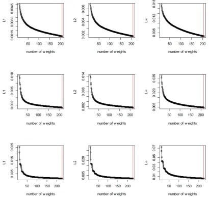
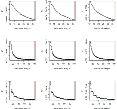
method described in (5) for a given N. The resulting Dp(N) value is plotted for
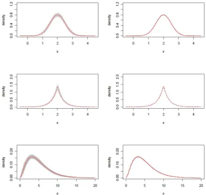
N = 2,3, . . . , Nmax. Figures 1 and 2 presents the plot forn = 500 andn= 20,000,
respectively, and in each case the red vertical line shows the selected value of N
using three Lp criteria for each of the three underlying distributions. Clearly, in
each of the cases the value of Dp(N) stabilizes for sufficiently large values of N.
As a matter of practical convenience, (in order to save on computing time), we use
the following ad-hoc stopping rule for N > m/2: set a small value δ >0 and stop
if |Dp(N)−Dp(N −1)|< δDp(N −1) or if N =Nmax. In our simulation studies,
we fix δ= 0.001 and Nmax =n/2 for all scenarios.
In Figures 1 and 2, we clearly see that in all scenarios (that we have explored),
the selected ˆNpdo not vary much withp. AsD∞is the strongest norm and provides
visually pleasing estimates, for rest of our empirical studies we set ˆN = ˆN∞.
3.2
Comparing AD based estimate with MLE
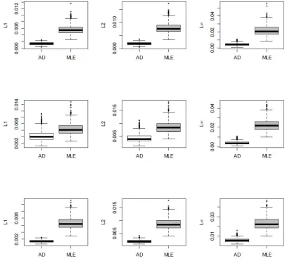
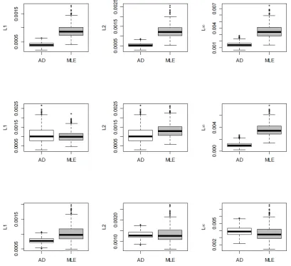
Next, we compare the performance of the estimates obtained by the proposed AD
method with MLE. Specifically, we generate data from a chosen latent parametric
distribution, use a set of equally spaced cut-points to generate a sample ofnordinal
values and then compute threeDp metrics to compare the fits obtained by AD and
MLE by repeating the data generation 500 times. Note that the MLE is obtained
by maximizing (2) and then ˆfk =F0(ck,θˆ)−F0(ck−1,θˆ), where ˆθ = arg maxL(θ).
In comparison, when using the AD method we do not use the known parametric
form to compute ˆfk, but rather use the form given in (3), after estimatingθ using
(5), and then select N using the criteria described in the previous section. As it
is well known that MLE provides biased estimates under misspecified models, we
do not present results for such unfavorable scenarios. However, our proposed class
of mixture of scaled Beta densities are robust against any underlying continuous
density.
simulations of MLE and AD for two different sample sizes and three different
underlying distributions. The AD method performs remarkably well compared to
MLE considering the fact the former does not uses the known parametric form of
the latent distribution. At n= 20,000 the AD method does as well as MLE, even
as the latter has well-known large sample consistency properties. Additionally,
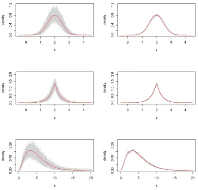
we also present the 500 estimated densities in Figures 5 and 6 corresponding to
n = 500 and 20,000. The red curve represents the true underlying latent density in
each case. It is evident when sample size is not large, the AD-based method density
estimates have larger variances compared to MLE, but it should be noted that AD
method here does not make use of known form the true density. However, when
sample size is sufficiently large, we find that AD based method produces density
estimates which are almost as good as MLE based density estimates.
Thus, from all of the simulated data scenarios we find that the AD method
provides a reasonably good estimate of the latent distribution even compared to
MLE (which make use of known parametric form of the latent distribution) and
the AD method is almost automatic (in terms of selectingN) and adaptive to any
shape (e.g., symmetric, skewed, etc.) of the underlying latent density. Moreover,
we find that the AD method is computationally stable being based on QP methods,
as compared to nonlinear optimization that is required for the MLE method. Next,
we illustrate the AD method for a few real data cases where the MLE method is not
readily applicable as the shape of the underlying density appears to be multimodal
and there is no obvious way to guess a suitable parametric family.
4
Estimation of latent distributions for ARMS
data
We demonstrate the application of the AD method using the household section
U.S. Department of Agriculture’s primary source of information on the financial
condition, production practices, and resource usage of the nation’s farm
house-holds1. The household section of this dataset is widely to study the behavior of
U.S. farm families with regard to decisions about off-farm employment, as well as
the household’s off-farm income, expenditures, debt, and investment. The entire
household section is value coded for ordinal responses to the survey questions.
Many of the variables in ARMS household section have distributions that do not
readily fit to a parametric family. This makes estimation of the underlying latent
density a challenge using standard parametric techniques.
The ARMS data contain cut-points, with each upper and lower cut-point
rep-resenting an interval on the dollars scale. Each interval is assigned to a specific
value code. The range of value codes is between 1 and 34 (a few variables can take
negative value codes and thus have a range of -34 to 34). An important detail is
that the dollar value intervals get wider as the value codes increase.
The 34th cut-point presents an issue because it is unbounded from above. To
address this issue, we replace the last cut-point by assigning a value equal to the
sum of the 33rdcut-point and the standard deviation of the cut-points. We do the
same with distributions unbounded from below. Before applying the AD method
we take either a natural logarithm or rth power (r ∈ (0,1]) transformation of the
cut-points for numerical stability. The rth power transformation is advantageous
because it has a finite continuous limit at zero. We make use of this fact when
estimating the latent distribution for data sets with a large proportion of zeros.
1For more information on the uses of ARMS see: http://www.ers.usda.
gov/data-products/arms-farm-financial-and-crop-production-practices/
4.1
Empirical results
We fit three different variables from the ARMS household section. These variables
are: (i) R1113 previous year total farm sales, (ii) R1105 household food expenses,
and (iii) R1114 previous year net operating income. The first two variables have
a [0,∞) support, while the last variable has a (-∞,∞) support. We also note that
the first two variables have a substantial number of zeroes in the data, between 8
and 10 percent. We explore the use of r= 1/5,1/7,1/9 and 1/11 power
transfor-mations along with the log-transformation on the cut-points before applying the
AD method. From our empirical studies (not shown here) we find that r = 1/9
provides best fit in terms of minimizing the D∞ metric. All the results displayed
in this section are based on first transforming the cut-points to ther = 1/9 power
and then applying the AD method to select N using the D∞ metric.
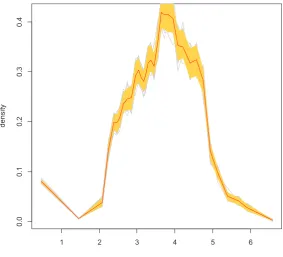
As shown in Figures 7-9, the estimated latent distributions of these variables
are clearly not belong to any well-known parametric family. In each of these figures
we present the AD based estimated density with 95% confidence bands obtained by
100 bootstrap samples of the data. These examples clearly depicts the versatility
and adaptivity of the proposed class of models and the AD method of estimation.
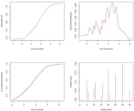
In Figures 10-12 we present (a) the estimated CDF of the underlying true
distribution, (b) estimated probabilities ( ˆfk( ˆN)’s as defined in Section 2.l) against
the empirical frequencies (fk’s), (c) estimated cumulative probabilities against the
empirical cumulative probabilities and (d) the estimated weights. Again all of these
plots clearly shows the adaptivity of the proposed class of scaled Beta mixtures by
zeroing out the estimated weights in portions where the underlying latent density
has very low mass (e.g., compare the magnitude and number of estimated weights
in Figures 10 and 11).
The AD method does well at finding the sharp peak in the distribution of
household food expenditures in Figure 8. It also does well with the multiple modes
seen in Figures 7 and 9. For previous year total farm sales the mass of zeroes are
against the lower bound of the support. Still, the AD method is able to find the
peak of the zeros, as shown in Figure 7. For each distribution, our default stopping
criteria choose a value of between 80 and 110 weights.
5
Conclusion
We presented a method for estimating the latent density of ordinal data. This
method uses a mixture of weighted Beta distributions, known as Bernstein
Poly-nomials, combined with information on the latent distribution provided by the
cut-points to estimate the latent density. We present three criteria for evaluating
the fit of the latent density based on measuring the distance between the
empir-ical distribution and the estimated distribution, evaluated at the cut-points. A
simulation study and empirical data examples demonstrate the effectiveness of our
method compared to popular maximum likelihood approaches. We also provide
a stopping criteria for choosing the optimal number of weights. An R function is
available by request. It is also available in the online supplementary material.
One limitation of our approach is the loss of efficiency by not constricting the
shape of the latent density to unimodal, when this fact is known. As shown in
Turnbull and Ghosh (2014), this can give the AD method more power in finding
the correct density. However, the trade-off is that our approach can also estimate
multimodal and other odd-shaped densities. Future work could look at a more
rigorous criteria for determining the optimal number of weights.
References
[1] Agresti, Alan, and Maria Kateri. Categorical Data Analysis. Springer Berlin
[2] Albert, James H., and Siddhartha Chib. “Bayesian analysis of binary and
polychotomous response data.” Journal of the American Statistical
Associa-tion 88.422 (1993): 669-679.
[3] Anderson, Theodore W., and Donald A. Darling. “ Test of goodness of fit.”
Journal of the American Statistical Association 49.268 (1954): 765-769.
[4] Babu, G. Jogesh, Angelo J. Canty, and Yogendra P. Chaubey. “Application
of Bernstein polynomials for smooth estimation of a distribution and density
function.”Journal of Statistical Planning and Inference 105.2 (2002): 377-392.
[5] Flora, David B., and Patrick J. Curran. “An empirical evaluation of
alterna-tive methods of estimation for confirmatory factor analysis with ordinal data.”
Psychological methods 9.4 (2004): 466-491.
[6] Ghosal, Subhashis. “Convergence rates for density estimation with Bernstein
polynomials.” Annals of Statistics 29.5 (2001): 1264-1280.
[7] Johnson, Valen E., and James H. Albert. Ordinal Data Modeling. Springer
Science & Business Media, 2006.
[8] Kottas, Athanasios, Peter Mller, and Fernando Quintana. “Nonparametric
Bayesian modeling for multivariate ordinal data.” Journal of Computational
and Graphical Statistics 14.3 (2005): 610-625.
[9] Leblanc, Alexandre. “A bias-reduced approach to density estimation using
Bernstein polynomials.”Journal of Nonparametric Statistics 22.4 (2010):
459-475.
[10] Leblanc, Alexandre. “On estimating distribution functions using Bernstein
polynomials.” Annals of the Institute of Statistical Mathematics 64.5 (2012a):
[11] Leblanc, Alexandre. “On the boundary properties of Bernstein polynomial
es-timators of density and distribution functions.” Journal of Statistical Planning
and Inference 142.10 (2012b): 2762-2778.
[12] Lorentz, G. G.Bernstein Polynomials Chelsea Publishing Series. Chelsea Pub
Co., New York (1986).
[13] Mant´e, Claude. “Iterated Bernstein operators for distribution function and
density estimation: Balancing between the number of iterations and the
poly-nomial degree.”Computational Statistics & Data Analysis 84 (2015): 68-84.
[14] McCullagh, Peter. “Regression models for ordinal data.” Journal of the Royal
Statistical Society. Series B (Methodological) 42.2 (1980): 109-142.
[15] Parzen, Emanuel. “On estimation of a probability density function and mode.”
The Annals of Mathematical Statistics 33.3 (1962): 1065-1076.
[16] Petrone, Sonia. “Bayesian density estimation using Bernstein polynomials.”
Canadian Journal of Statistics 27.1 (1999): 105-126.
[17] Petrone, Sonia, and Larry Wasserman. “Consistency of Bernstein
polyno-mial posteriors.”Journal of the Royal Statistical Society: Series B (Statistical
Methodology) 64.1 (2002): 79-100.
[18] Shah, D. A., and L. V. Madden. ”Nonparametric analysis of ordinal data in
designed factorial experiments.”Phytopathology 94.1 (2004): 33-43.
[19] Tamhane, Ajit, Bruce Ankenman, and Ying Yang. “The beta distribution as a
latent response model for ordinal data (I): estimation of location and dispersion
parameters.” Journal of Statistical Computation and Simulation 72.6 (2002):
[20] Turnbull, Bradley C., and Sujit K. Ghosh. “Unimodal density estimation using
Bernstein polynomials.”Computational Statistics & Data Analysis 72 (2014):
13-29.
[21] Vitale, Richard A. “A Bernstein polynomial approach to density function
estimation.”Statistical Inference and Related Topics 2 (1975): 87-99.
[22] Winship, Christopher, and Robert D. Mare. “Regression models with ordinal
Figure 1: Plot of Dp(N) vs. N for p = 1,2,∞ when n = 500. First row cor-responds normal, second corcor-responds to Laplace and third row corcor-responds to
Figure 2: Plot of Dp(N) vs. N for p = 1,2,∞ when n = 20,000. First row corresponds normal, second corresponds to Laplace and third row corresponds to
Figure 3: Boxplots of Dp(N) comparing AD and MLE for p = 1,2,∞ when n = 500. First row corresponds normal, second corresponds to Laplace and third row
Figure 4: Boxplots of Dp(N) comparing AD and MLE for p = 1,2,∞ when n =
20,000. First row corresponds normal, second corresponds to Laplace and third
Figure 5: Estimates of latent densities by using the MLE when n = 500 (in
column 1) and n = 20,000 (in column 2). First row corresponds normal, second
Figure 6: Estimates of latent densities by using the AD whenn = 500 (in column 1)
and n = 20,000 (in column 2). First row corresponds normal, second corresponds
1 2 3 4 5 6
0
.0
0
.1
0
.2
0
.3
0
.4
root.mid.points
d
e
n
si
ty
Figure 7: Estimated latent density for Previous Year Total Farm Sales using the
AD method. The ˆN = 150 was obtained using the D∞ criteria and r= 1/9 power
1 2 3 4 5 6
0
.0
0
.5
1
.0
1
.5
2
.0
root.mid.points
d
e
n
si
ty
Figure 8: Estimated latent density for Household Food Expenditures using the
AD method. The ˆN = 104 was obtained using the D∞ criteria and r= 1/9 power
-5 0 5
0
.0
0
.1
0
.2
0
.3
0
.4
0
.5
root.mid.points
d
e
n
si
ty
Figure 9: Estimated latent density for Previous Year Net Operating Income using
the AD method. The ˆN = 150 was obtained using the D∞ criteria and r = 1/9
1 2 3 4 5 6 0 .2 0 .4 0 .6 0 .8 1 .0 root.cut.points e st ima te d cd f
2 3 4 5 6
0 .0 1 0 .0 2 0 .0 3 0 .0 4 0 .0 5 0 .0 6 root.mid.points e mp ir ica l p ro b a b ili ty
2 3 4 5 6
0 .2 0 .4 0 .6 0 .8 1 .0 root.cut.points cu m u la ti v e p ro b a b ili ty
0 5 10 15 20 25 30 35
0 .0 0 0 .0 5 0 .1 0 0 .1 5 0 .2 0 weight index w e ig h t v a lu e
Figure 10: Estimated CDF, empirical and cumulative probabilities, and estimated
weights for Previous Year Total Farm Sales using the AD method. The ˆN = 150
was obtained using the D∞ criteria and r = 1/9 power transformation was used
−1 0 1 2 3 4 5 6 0 .0 0 .2 0 .4 0 .6 0 .8 1 .0 root.cut.points e st ima te d cd f
0 1 2 3 4 5 6
0 .0 0 0 .0 5 0 .1 0 0 .1 5 0 .2 0 root.mid.points e mp ir ica l p ro b a b ili ty
1 2 3 4 5 6
0 .0 0 .2 0 .4 0 .6 0 .8 1 .0 root.cut.points cu m u la ti v e p ro b a b ili ty
0 20 40 60 80 100
0 .0 0 .1 0 .2 0 .3 0 .4 0 .5 0 .6 0 .7 weight index w e ig h t v a lu e
Figure 11: Estimated CDF, empirical and cumulative probabilities, and estimated
weights for Household Food Expenditures using the AD method. The ˆN = 104
was obtained using the D∞ criteria and r = 1/9 power transformation was used
−6 −4 −2 0 2 4 6 0 .2 0 .4 0 .6 0 .8 1 .0 root.cut.points e st ima te d cd f
−6 −4 −2 0 2 4 6
0 .0 0 0 .0 2 0 .0 4 0 .0 6 0 .0 8 0 .1 0 root.mid.points e mp ir ica l p ro b a b ili ty
−6 −4 −2 0 2 4 6
0 .4 0 .6 0 .8 1 .0 root.cut.points cu m u la ti v e p ro b a b ili ty
0 20 40 60 80 100
0 .0 0 .1 0 .2 0 .3 0 .4 0 .5 0 .6 weight index w e ig h t v a lu e
Figure 12: Estimated CDF, empirical and cumulative probabilities, and estimated
weights for Previous Year Net Operating Income using the AD method. The
ˆ
N = 150 was obtained using the D∞ criteria and r = 1/9 power transformation