DOI: 10.1534/genetics.108.088542
AMBIENCE: A Novel Approach and Efficient Algorithm for Identifying
Informative Genetic and Environmental Associations With
Complex Phenotypes
Pritam Chanda,* Lara Sucheston,
†,‡Aidong Zhang,* Daniel Brazeau,
†Jo L. Freudenheim,
§Christine Ambrosone
‡and Murali Ramanathan**
,1*Department of Computer Science and Engineering,†Department of Biostatistics,§Department of Social and Preventive Medicine and **Department of Pharmaceutical Sciences, State University of New York, Buffalo, New York 14260 and‡Department of Cancer
Prevention and Control, Roswell Park Cancer Institute, Buffalo, New York 14263 Manuscript received March 9, 2008
Accepted for publication August 4, 2008
ABSTRACT
We developed a computationally efficient algorithm AMBIENCE, for identifying the informative variables involved in gene–gene (GGI) and gene–environment interactions (GEI) that are associated with disease phenotypes. The AMBIENCE algorithm uses a novel information theoretic metric called phenotype-associated information (PAI) to search for combinations of genetic variants and environmental variables associated with the disease phenotype. The PAI-based AMBIENCE algorithm effectively and efficiently detected GEI in simulated data sets of varying size and complexity, including the 10K simulated rheumatoid arthritis data set from Genetic Analysis Workshop 15. The method was also successfully used to detect GGI in a Crohn’s disease data set. The performance of the AMBIENCE algorithm was compared to the multifactor dimensionality reduction (MDR), generalized MDR (GMDR), and pedigree disequilibrium test (PDT) methods. Furthermore, we assessed the computational speed of AMBIENCE for detecting GGI and GEI for data sets varying in size from 100 to 105variables. Our results demonstrate that the AMBIENCE information theoretic algorithm is useful for analyzing a diverse range of epidemiologic data sets containing evidence for GGI and GEI.
T
HE risk of developing many chronic diseases such as cancer, cardiovascular diseases, autoimmune dis-eases, and mental disorders may involve interactions among a number of genetic, endogenous, and exoge-nous environmental factors (Shieldsand Harris2000; Talmudand Stephens2004; Caspiand Moffitt2006; Ambrosoneet al. 2007; Arasonet al. 2007). The success-ful identification of critical gene–environment interactions (GEI) may provide the scientific basis for preventative public health measures to help individuals with par-ticular genetic susceptibilities reduce their exposure to disease risk-increasing environmental variables. Better analytical methods for detecting GEI can facilitate iden-tification of environmental factors capable of modifying the effects of genetic risk factors on disease outcome.Advances in high-throughput genotyping methods have made generating dense genetic maps of the hu-man genome for epidemiological studies feasible. The additional information from these methods improves the prospects for uncovering the interactions underly-ing genetic etiology of multifactorial diseases. With re-spect to study design, identification of gene–gene
interactions (GGI) is important for follow-up sequenc-ing studies and results from GEI analyses can help in reducing confounding in replication studies by ensur-ing relevant informative environmental variables are collected. Statistical GGI and GEI analyses can also pro-vide epro-vidence in support of specific disease mechanisms. Unfortunately, there is a paucity of comprehensive ap-proaches that can conduct higher-order GGI and GEI analyses on a genomewide scale (Purcellet al. 2007).
Although there is considerable need for GGI and GEI analyses to understand the genetics of many diseases, there are unique scientific challenges attributable to the potential involvement of multiple genetic and environ-mental factors in the etiology of the disease, the high dimensionality of the data sets from genomewide studies, and combinatorial explosion. As the number of ways of selecting a subset of K genetic or environ-mental variables for assessing interactions fromNsuch variables is equal toNK, the binomial coefficient or N-choose-Kfunction, the number of interactions increases with extraordinary rapidity. This combinatorial growth makes it computationally difficult, if not impossible, to exhaustively assess the full range of genetic and envi-ronment variables for potential interactions associated with diseases in epidemiologic studies. As an example,
1Corresponding author:427 Cooke Hall, Department of Pharmaceutical
Sciences, State University of New York, Buffalo, NY 14260. E-mail: [email protected]
there are 1.6731011possible three-way GGIs for a data
set with 10,000 SNPs. If the calculations for each GGI could be accomplished in 1 msec, the computation time required would be.5 years.
The multifactor dimensionality reduction (MDR) technique (and software) for identifying and analyzing GEI was developed by Ritchie and colleagues (Ritchie
et al. 2001; Hahnet al. 2003; Mooreet al. 2006). MDR is
based on nonparametric multifactor models and allows statistical and cross-validation analysis of GGI and GEI for balanced case–control and discordant sib-pair de-signs (Ritchieet al. 2001, 2003; Hahnet al. 2003; Bush et al. 2006). MDR uses constructive induction wherein the dimensionality of the multilocus genotype is system-atically reduced by pooling into high and low risk groups (Mooreet al. 2006). The MDR method has been extended to unbalanced data sets (Velezet al. 2007) and a theoretical analysis of MDR has shown the similarity of the MDR classifier to the naive Bayes classifier (Hahn and Moore2004). The MDR approach has been used to study GEI in atrial fibrillation, autism, and diabetes mellitus (Choet al. 2004; Tsaiet al. 2004; Maet al. 2005; Motsingeret al. 2006). The recently proposed gener-alized MDR (GMDR) method employs the genergener-alized linear model (GLM) framework for scoring in conjunc-tion with MDR for dimensionality reducconjunc-tion (Louet al. 2007). GMDR enables inclusion of covariates and handles both discrete and continuous traits in popula-tion-based study designs. GMDR employs the same risk-pooling, dimensionality reduction strategy as MDR and yields the original MDR as a special case when covariates are not present and the trait under investigation is binary
(Louet al. 2007). However, despite availability of a more
efficient parallel computing implementation (Bushet al. 2006), MDR and its variants, including GMDR, are computationally intensive, especially when .10 poly-morphisms need to be evaluated (Ritchieet al. 2001).
One approach that allows hypotheses of specific types of GGI and GEI to be tested is the pedigree disequilib-rium test (PDT) (Martinet al. 2000) as implemented in the software program UNPHASED (v3.10) (Dudbridge 2003). Although designed for family-based studies (in-cluding case–parent trios and affected sibling pairs study designs), the PDT approach is flexible enough for the analysis of associations in case–control study designs. Likelihood-ratio tests (LRT) can be built to test synergistic epistasis,i.e., when the effect of the combi-nation of two alleles at two different diallelic loci is greater than the additive effects of the loci alone. The LRT can also be built to test for effect measure modifi-cation, which occurs when varying levels of an environ-mental risk factor modify the risk ratio of the genotype. The PDT has the appeal of a formal statistical frame-work: the hypothesis tests for synergistic epistasis and effect measure modification are statistical tests of in-teraction. It is flexible with regard to study design and can accommodate missing data. The PDT approach has
been used to extend the MDR to allow analysis of families (Martinet al. 2006). However, the computational challenges remain.
The available methods are computationally prohibi-tive for analyzing interactions in genomewide data and there is a need for novel methodology. Information theoretic methods are among the most promising approaches for enhancing single-nucleotide polymor-phism (SNP) analysis, GGI and GEI analysis, and vi-sualization (Liu and Lin 2005; Bhasi et al. 2006a,b;
Moore et al. 2006). Information-theoretic approaches
have well-developed theory and are versatile and genetic model independent but only limited research on leveraging these strengths into analytical strategies for GGI and GEI has been done. Several reports have used the Kullback–Leibler divergence (KLD) for genetic analysis (Smithet al. 2001; Andersonand Thompson 2002; Rosenberget al. 2003; Liuand Lin2005). The KLD is a measure of the ‘‘distance’’ between two distri-butions because it measures the inefficiency of assum-ing that the distribution isqwhen the true distribution
isp. In genetic analyses, the most frequent application
of the KLD has been for two-group comparisons such as those used to evaluate ancestry informative markers
(Smith et al. 2001; Anderson and Thompson 2002;
Rosenberget al. 2003). However, the KLD has also been proposed as a multilocus linkage disequilibrium (LD) measure to enable identification of TagSNPs (Liuand Lin 2005) and our group has adapted the KLD for analytical visualization (Bhasiet al. 2006a,b). Informa-tion theory statistics employing entropy-based statistics have been proposed for genomewide data analysis to test for allelic association with a phenotype (Zhaoet al. 2005, 2007; Liet al. 2007). Entropy-based methods for two-locus interactions have also been proposed recently and were found to confirm the negative epistasis be-tween sickle cell anemia and a-thalassemia genetic variations against malaria (Donget al. 2007).
Information theoretic approaches offer many potent capabilities and advantages for GGI and GEI analyses. These approaches utilize extensions of the KLD to measure complex multivariate dependencies among genetic variations and environmental factors without complex modeling. In our previous report, we devel-oped an approach for GGI and GEI visualization and identification that utilizes two established and comple-mentary information-theoretic metrics, the K-way in-teraction information (KWII) and the total correlation information (TCI) for GEI and GGI analyses (Chanda et al. 2007). We demonstrated that the KWII spectra of a data set are capable of identifying critical interactions and contain information that can be utilized to infer the biological mechanisms generating the interactions.
The goals for this research were to substantively extend the concepts and methods developed in our earlier report (Chandaet al. 2007) by (i) developing a novel metric, the phenotype-associated information
(PAI) that is robust to the confounding effects of factors such as pairwise and higher-order LD and correlations between environmental variables, (ii) demonstrating that the PAI is a useful information theoretic metric for effectively screening GGI and GEI, and (iii) developing an algorithm AMBIENCE that employs the PAI metric to efficiently search the combinatorial space to identify the variables involved in the strongest interactions. The results from this work will enable the development of better methods for efficient, large-scale interaction analysis.
MATERIALS AND METHODS
Terminology and representation: The methods in this article are applicable to both GEI and GGI analyses and henceforth we simply use the term GEI to refer to both. The term GGI is used only when environmental variables are not present in a data set.
Definition of interaction: The KWII is a parsimonious, multi-variate measure of information gain, which is defined and described in detail below ( Jakulinand Bratko2004; Jakulin 2005). In our information theoretic framework, we use the KWII as the measure of interaction information for each variable combination. We operationally define that a positive KWII value for a variable combination indicates the presence of an interaction, negative values of KWII indicate the presence of redundancy, and a KWII value of zero denotes the absence ofK-way interactions.
This operational definition based on the KWII corresponds closely to but is not exactly the same as the formulation of statistical interactions in the context of logistic regression. For a succinct discussion of the concordance and differences with other definitions see Jakulin(2005).
Entropy:The entropy,H(X), of a discrete random variableX can be computed from the probabilities of p(x) using the formula
HðXÞ ¼ X
x
pðxÞlogpðxÞ:
K-way interaction information (KWII): For the three-variable case, the KWII is defined in terms of entropies of the individual variables,H(A),H(B), andH(C) and the entropies, H(AB),H(AC),H(BC), andH(ABC), of the combinations of the variables:
KWIIðA;B;CÞ ¼ HðAÞ HðBÞ HðCÞ1HðABÞ 1HðACÞ1HðBCÞ HðABCÞ:
For theK-variable case on the setn¼ fX1;X2; . . . ;XKg, the
KWII can be written succinctly as an alternating sum over all possible subsetsTofnusing the difference operator notation of Han(1980):
KWIIðnÞ[X
T4n
ð1ÞjnjjTjHðTÞ:
The number of variablesKin a combination is called the order of the combination. The KWII represents the gain or loss of information due to the inclusion of additional variables in the model. It quantifies interactions by representing the informa-tion that cannot be obtained without observing allKvariables at the same time (McGill 1954; Fano 1961; Jakulin and
Bratko2004; Jakulin2005). The KWII of a given combina-tion of variables is a parsimonious interaccombina-tion metric. It does not contain contributions arising from the KWII of other lower-order combinations of these variables.
In the bivariate case, the KWII is always nonnegative but in the multivariate case, KWII can be positive or negative. The interpretation of KWII values is intuitive because positive values indicate synergy between the variables, negative values indicate redundancy between variables, and a value of zero indicates the absence ofK-way interactions.
TCI:For the three-variable case, the TCI (Watanabe1960) is defined in terms of entropies of the individual variables H(A),H(B), andH(C) and the entropy of the joint distribu-tionH(ABC):
TCIðA;B;CÞ ¼HðAÞ1HðBÞ1HðCÞ HðABCÞ:
For theK-variable case on the setn¼ fX1;X2; . . . ;XKg, the
TCI can be expressed as the difference between the entropies of the individual variablesH(Xi) and the entropy of the joint distributionH(X1X2. . .XK):
TCIðX1;X2;. . .;XKÞ ¼
XK
i¼1
HðXiÞ HðX1X2;. . .XKÞ:
The TCI is the amount of information shared among the variables in the set; equivalently, it can be viewed a general measure of dependency. A TCI value that is zero indicates that knowing the value of one variable tells you nothing about the others,i.e., that the variables are independent. The maximal value of TCI occurs when one variable is completely re-dundant with the others;i.e., knowing one variable provides complete knowledge regarding all the others.
Phenotype-associated information: The PAI is obtained from the TCI, which represents the overall dependency among the genetic and environmental variables and the phenotype variable by removing the TCI contributions repre-senting the interdependencies among the genetic and envi-ronmental variables. The interdependencies among variables can be caused by factors such as LD or by a common source for multiple pollutant exposures. Accordingly, PAI is defined by
PAIðX1;X2;. . .;XK;PÞ
¼TCIðX1;X2;. . .;XK;PÞ TCIðX1;X2;. . .;XKÞ:
In the above equation, the genetic and environmental variables are denoted by theX1,X2,. . .,XK, and the phenotype
variable is denoted by P. In the PAI definition, the TCI(X1, X2,. . .,XK,P) term represents the overall dependency among
the genetic and environmental variables and the phenotype whereas the TCI(X1, X2,. . ., XK) term represents the
inter-dependencies among the genetic and environmental variables in the absence of the phenotype variable.
The KWII is the more valuable information metric because it is a parsimonious measure of interaction for the variable combination of interest alone and does not contain contribu-tions from lower-order interaccontribu-tions. However, KWII computa-tions on the entire combinatorial space are computationally intractable because they require the entropies of all subsets. In addition, the KWII cannot be used for hill-climbing algorithms because it takes on both positive and negative values. Thus, it is necessary to concomitantly address the biological complex-ities and computational efficiency in GEI analysis.
Only individual and joint entropies are needed for TCI calculations, making it computationally far more tractable than the KWII. TCI (and PAI) on the other hand, is always greater than or equal to zero and increases monotonically with increased combination size [i.e., TCI(A, B, C, D) $TCI(A, B,C)], making it potentially suitable for hill-climbing algo-rithms. Unfortunately because the TCI is a general measure of dependency, it is sensitive to factors that cause correlations and interredundancies among variables such as LD.
The PAI is an effective approach to overcoming these GEI-associated biological and computational issues.
Properties of the PAI:We developed the PAI to obtain a TCI-based measure that is robust to the confounding effects of biological dependencies such as LD.
PAI, TCI, and KWII are each equal to mutual information for single variable associations with the phenotype. However, for higher-order combinations, the PAI definition removes the TCI for pairwise and multimarker LD among the genetic variables and similar uninformative dependencies among environmental variables from the overall TCI. As a conse-quence, the PAI does not have the biological drawbacks such as sensitivity to LD and to correlations among environmental variables that limit the usefulness of the TCI.
The PAI also offers the computational efficiency associated with TCI calculations. The PAI is always greater than or equal to zero (see appendix) and increases monotonically with increased combination size (seeappendix), making it very suitable as the basis for hill-climbing algorithm design.
The PAI contains useful information regarding the KWII of the genetic and environmental variables and the phenotype. By derivation (seeappendix), it can be shown that
PAIðX1;X2;. . .;XK;PÞ ¼
X
T4n
KWIIðT;PÞ:
This equation demonstrates that the PAI is the cumulative phenotype-associated synergy present in all subset combina-tions of the variablesX1,X2,. . .,XKandP. It is important to
note that each component of the KWII is free of the confounding effects of other combinations.
We use the PAI to identify the interesting regions in the combinatorial space and then compute the KWII for the reduced combinatorial space. This is a ‘‘greedy search’’ strategy that avoids combinatorial explosion because it does not conduct GEI analysis for every possible combination.
The AMBIENCE algorithm:The AMBIENCE algorithm is computationally much more efficient than the exhaustive search (EXS) approach used in our earlier report (Chanda et al. 2007) to compute KWII for all possible SNP combina-tions, which requires exponential time. The pseudocode for AMBIENCE is shown in Figure 1.
The AMBIENCE algorithm employs the PAI to search for combinations of genetic variations and environmental varia-bles related to the disease phenotype. Let X¼ fX1;X2;. . .;Xng be the set of all genetic/environmental
variables andPbe the disease phenotype variable. The inputs to the AMBIENCE algorithm areX,P, and algorithm param-etersuandt, which represent the number of combinations
retained in the iterations of the search and the number of iterations, respectively. The parametertdetermines the high-est order of variable combination detected.
We start by calculating PAIðXi;PÞ"i21. . .n. We retain the topucombinations with the highest values of PAI. Let this set of variables be denoted byS1. In the next step, we calculate
PAIðXi;Xj;PÞ"Xi2S1;"j21. . .n;ðj 6¼iÞ. We again retain
the topucombinations with the highest values of PAIðXi;Xj;PÞ in set S2. The above steps are repeated t times. Thus, we
greedily search for combinations containing up totvariables that have higher values of PAI. These combinations identify regions in the combinatorial space that have combinations with strongly interacting variables. Finally, for each combina-tionCidentified by the above search steps, we calculate the KWIIðn;PÞ"n4Cto identify the most parsimonious strongly interacting combinationsfn;Pg.
Additional analyses of time complexity and evaluations of computational speed for AMBIENCE are presented in results.
Simulations for case studies:Simulated data sets were used to critically assess the effectiveness of the PAI metric to correctly identify the interacting variables. We selected the interaction model for case study 1 from our earlier article
(Chanda et al. 2007) because it had necessary levels of
complexity and also contained nuanced GEI patterns that could provide a challenging test for evaluating the PAI. The model for case study 2 was constructed to be more complex than case study 1 and was motivated by genetic, environmen-tal, and biomarker variables implicated in congestive heart disease. The simulations assumed complete penetrance.
A population of 50,000 individuals with randomly varying genotypes and environmental exposures consistent with the underlying GEI models was generated for each of the case studies. The case–control study design was assumed. From the population of 50,000 individual genotypes, a sample of 500 cases and 500 controls was randomly selected. The value 1 was used to represent cases and 0 was used for controls. The standard deviations due to sampling were calculated from 100 independent repetitions of this procedure.
Case studies 1A and 1B:The underlying GEI model for case studies 1A and 1B is summarized in Figure 2A. The simulated data for case studies 1A and 1B consisted of four environmen-tal variables, E1–E4, and six SNP variables, SNP 1–SNP 6. The environmental variables E1 and E2 were assumed associated with the disease phenotype whereas E3 and E4 were assumed to be uninformative. The environmental variables E1 and E3 were assumed to have two states, low exposure (assigned value¼
L) and high exposure (assigned value¼H) that were treated as categorical. The environmental variables E2 and E4 were assumed to have three states, low exposure (assigned value¼
L), medium exposure (assigned value¼M), and high expo-sure (assigned value¼H) that were also treated as categorical. The percentages of subjects in low- and high-exposure groups of E1 and E3 were each 50%; the percentages of subjects in low-, intermediate-, and high-exposure groups of E2 and E4 were 33.33% each, respectively. The disease was modeled to occur for various combinations of exposure to the environ-mental variables E1 and E2 via interactions with alleles for two SNPs, SNP 1 and SNP 2. To mimic an additive genetic model, the values 1, 2, and 3 were used to represent the homozygous state for the major allele, the heterozygous genotype, and the homozygous state for the minor allele, respectively, for all six SNP variables. The more common and less common (disease) alleles of SNP 1 and SNP 2 were assigned allele frequencies of 0.9 and 0.1, respectively. The other SNP variables, SNP 3–SNP 6, were uninformative and had allele frequencies of 0.5. All SNPs were assumed to be diallelic with the three possible geno-types in Hardy–Weinberg equilibrium. A binary phenotype
variable,C, representing case (assigned value¼1) or control (assigned value¼0) was used.
In both case studies 1A and 1B, the E1 and E2 variables were assumed to act independently of each other and the case phenotype value was assigned when combinations of the SNP genotypes and either environmental variable resulted in a case. In case study 1A, absence of LD among the SNP variables was assumed. In contrast, for case study 1B, the SNP variables SNP 3 and SNP 4 were assumed to be in LD (R2¼0.9) with each other.
Case study 2:This case study is summarized in Figure 2B and contains a complex combination of environmental variables, SNP variables, and biomarker variables that determine the disease phenotype.
The model for case study 2 consisted of four environmental variables, E1–E4, four SNP variables, SNP 1–SNP 4, and two biomarker variables B1 and B2. The overall risk of developing the disease phenotype was determined by contributions from three components termed (i) environmental risk component (risk E), (ii) the genetic risk component (risk G), and (iii) the biomarker risk component (risk B). The risk E component was assumed to have three states (H, high;M, medium; andL, low) whereas risk G and risk B were assumed to have two states (H and L). The SNP 1 variable interacted with the E1 and E2 environmental variables to determine the environmental risk component (risk E) of disease risk in Figure 2B. The gene– gene interactions between SNP 2 and SNP 3 variables de-termined the genetic risk component (risk G) of disease risk whereas interactions between the two biomarker variables, B1 and B2, determined risk B.
The environmental variables, E1 and E2, were disease associated whereas E3 and E4 were assumed to be uninforma-tive. The environmental variables E1 and E3 were each assumed to have two states, low exposure (assigned value ¼
L) and high exposure (assigned value¼H); the remaining environmental variables E2 and E4 each had an additional state of medium exposure (assigned value ¼ M). The per-centages of subjects in low- and high-exposure groups of E1 and E3 were each 50%; the percentages of subjects in low-, medium-, and high-exposure groups of E2 and E4 were each 33.33%, respectively.
Both biomarker variables, B1 and B2 were assumed associ-ated with the disease phenotype and were each assumed to have three states, low exposure (assigned value¼L), medium exposure (assigned value¼M), and high exposure (assigned value¼H). The percentages of subjects in the low-, medium-, and high-exposure groups of B1 and B2 were 33.33% each, respectively.
All four SNP variables were assumed to be diallelic with the three possible genotypes in Hardy–Weinberg equilibrium. The values 1, 2, and 3 were used to represent the homozygous state for the major allele, the heterozygous genotype, and the homozygous state for the minor allele, respectively, for all four SNP variables. The more common and less common (‘‘disease’’) alleles of SNP 1, SNP 2, and SNP 3 were assigned allele frequencies of 0.9 and 0.1, respectively. The remaining SNP variable SNP 4 was un-informative and had allele frequencies of 0.5.
A binary phenotype variable,C, representing case (assigned value ¼ 1) or control (assigned value ¼ 0) was used. The disease was modeled to occur for various combinations of
Figure 1.—Pseudocode for the AMBIENCE
exposure to the environmental variables E1 and E2 via interactions with the biomarker variables B1 and B2 and alleles for three SNPs, SNP 1, SNP 2, and SNP 3. Variables E1, E2, and SNP 1 interact to affect the environmental risk E of the disease. Variables SNP 2 and SNP 3 interact to affect the genetic risk G of the disease. Variables B1 and B2 interact to affect the biomarker risk B of the disease.
Examples of prototypical environmental variables in con-gestive heart disease are inflammation and smoking. Bio-markers that are predictive of congestive heart disease risk include factors such as C-reactive peptide and blood choles-terol levels in serum.
Visualization of GEI:Results are summarized graphically as KWII, TCI, and PAI ‘‘spectra’’ as previously described (Chandaet al. 2007). These spectra are bar plots with KWII, TCI, or PAI on the x-axis and the corresponding variable combinations on they-axis. The variable combinations on the y-axis were grouped according to the number of variables involved in the combinations;i.e., the one-variable-containing combinations, two-variable-containing combinations, and three-variable-containing combinations were each placed in separate groups. Within each group, the combinations were arranged in ascending order so that specific variable combi-nations of interest could be easily found.
Analysis of public domain data sets:GEI analysis of Genetic Analysis Workshop 15 data:The data corresponding to problem 3 of Genetic Analysis Workshop 15 (GAW15) were obtained from the GAW site (http://www.gaworkshop.org/gaw15data. htm) and used with permission.
These data consist of 100 replicates of simulated data that are modeled after the rheumatoid arthritis (RA) data. Michael Miller and his colleagues generated the data (Miller et al. 2007) and the following data description was obtained from the web site http://genetsim.org/gaw15/answers/. Each
rep-licate includes 1500 nuclear families each with two parents and an affected sib pair and 2000 unrelated controls. The data contain three types of autosomal markers: (i) 730 micro-satellite markers with an average spacing of 5 cM, (ii) 9187 SNPs distributed on the genome to mimic a 10K SNP chip set, and (iii) 17,820 SNPs on chromosome 6. The data include map information, with lists of markers and their locations, and simulated family, marker, and phenotype data. The HLA DR genotype was also available and the phenotype/covariate data included rheumatoid arthritis affection status, age at ascer-tainment, lifetime smoking, anticyclic citrullinated peptide antibody (anti-CCP), immunoglobulin M (IgM), severity, age at onset, and age at death.
This simulated data set mimics the epidemiology and familial pattern of RA, a complex genetic disease in which it is hypothesized that several loci contribute to disease suscep-tibility. As summarized in Table 1, the data set models in-teractions of nine loci: C, DR, and D on chromosome 6, A on chromosome 16, B on chromosome 8, E on chromosome 18, F on chromosome 11, and G and H on chromosome 9. In ad-dition, sex, age, smoking status, anti-CCP measure, IgM mea-sure, severity, DR allele from father, DR allele from mother, age at onset, and age at death are included as covariates. The biomarkers, anti-CCP measures, and IgM measures are de-fined for the cases only. All SNP loci are diallelic and alleles are coded as 1 and 2.
For our analysis, which aimed to evaluate the effectiveness of AMBIENCE, we used the set of 9187 SNPs along with sex, age, and smoking status as covariates. We used all 100 rep-licates to obtain KWII and PAI values and the corresponding 95% confidence intervals for each combination of variables.
We refer to this data set as the ‘‘10K GAW15 data set.’’ The age, anti-CCP, and IgM variables, which are continuous measures, were discretized by simple binning into five intervals Figure2.—(A) The interaction model used to generate the data for case studies 1A and 1B. (B) The interaction model used to generate the data for case study 2. In A, the environmental variables E1 (with statesH,L) and E2 (with statesH,M, andL) in-dependently interact with two SNP variables, SNP 1 (with allelesA1andA2) and SNP 2 (with allelesB1andB2) to determine the
disease status (controls are indicated by 0 and cases are indicated by 1). In B, the disease occurs due to exposure to the environ-mental variables E1 and E2 via interactions with the biomarker variables B1 and B2 and alleles for three SNPs, SNP 1, SNP 2, and SNP 3. The environmental, genetic, and biomarker risks are denoted by E, G, and B, respectively. The asterisk in a genotype represents a ‘‘wild card’’ indicating that either allele is allowable. The uninformative variables are not shown.
of equal width. Although haplotype-phase information was provided, we chose to not include it and treated the data as unphased genotype data. We conducted separate analyses with RA affection status, anti-CCP, and IgM as phenotypes of interest. The IgM variable was included as a covariate in the analysis of anti-CCP as phenotype and vice versa. All the analyses were performed with AMBIENCE input parameter values ofu¼50 andt¼3.
GGI analysis of interactions in chromosome 5:We assessed the effectiveness of the KWII and TCI spectra for identifying key interactions in a genotype data set from Dalyet al. (2001) containing 103 SNPs spanning a 616-kb region of chromo-some 5q31 that has been linked to Crohn’s disease (Rioux et al. 2001; Onnieet al. 2006). The data set contains genotypes for 129 parent–child trios composed of 144 cases and 243 controls (Daly et al. 2001). For our analysis, SNPs whose genotypes were missing in$20% of subjects were excluded.
To obtain corresponding P-values for the KWII and PAI metrics, we permuted the case–control labels 5000 times. The family information in the data set was not considered in the permutation procedure.
Comparison to other competing approaches:We compared our approach to the MDR (Ritchie et al. 2001, 2003; Hahn et al. 2003; Bushet al. 2006), the GMDR (Louet al. 2007), and the PDT. The data were coded using an additive genetic model for all methods.
The AMBIENCE approach was compared to the MDR, GMDR, and PDT methods for GGI analysis on the Dalyet al. (2001) data set.
The ability of AMBIENCE to detect GEI in the presence of covariates was compared to that of the MDR, GMDR, and PDT methods on the GAW15 data set. For this head-to-head comparison of the performance of MDR, GMDR, and PDT to that of AMBIENCE on GAW15 data, we selected 100 SNPs from among the 9187 SNPs to create a smaller data set that could be analyzed by all three competing methods. We refer to this data set as the ‘‘100-SNP GAW15 data set.’’ Specifically, this data set included the covariates smoking, age, and sex and contained key informative loci and sufficient uninformative loci as follows: (i) SNPs 131–171 from the region of chromo-some 6 containing loci C, DR, and D; (ii) SNPs 30–32 from the region of chromosome 16 containing locus A; (iii) SNPs 438– 442 from the region of chromosome 8 containing locus B; (iv) SNPs 266–272 from the region of chromosome 18 containing locus E; (v) SNPs 387–391 from the region of chromosome 11 containing locus F; (vi) SNPs 181–196 from the region of chromosome 9 containing loci G and H; and (vii) the remaining 22 SNPs were selected randomly from the rest of
the 9187 SNPs. The RA affection status was used as the phenotype.
MDR method: The MDR implementation was downloaded from http://sourceforge.net/projects/mdr/. For MDR analy-sis of the Dalyet al. (2001) data set, samples missing genotypes at$10% of the SNPs were excluded followed by the exclusion of SNPs whose genotypes were missing in$10% of subjects.
The binary covariates, sex and smoking, and age (discre-tized as for the AMBIENCE analysis) in the 100-SNP GAW15 data set were input as additional markers for MDR analysis.
GMDR:The GMDR implementation was downloaded from http://www.healthsystem.virginia.edu/internet/addiction-genomics/software/gmdr.cfm#.
Pedigree disequilibrium test: The PDT (Martin et al. 2000) implementation in the software package UNPHASED v3.10
(Dudbridge2003) was used. The program PDTPHASE v3.07
(see http://www.mrc-bsu.cam.ac.uk/BSUsite/Publications/ Preprints/Unphased_manual.pdf) was used to perform tests of association of single SNPs and two-SNP haplotypes with disease status (Dudbridge 2003). The Daly et al. and the GAW15 data sets both included family information that was provided to the software program (Dalyet al. 2001; Miller et al. 2007). For the GAW15 data set (Milleret al. 2007), the covariates of age, sex, and smoking, which are available for both cases and controls, were included in the analysis.
Computational speed estimate: We tested the computa-tional efficiency of the AMBIENCE algorithm using the GAW 15 data set problem 3 (http://www.gaworkshop.org/gaw15data. htm).
We used the dense map of chromosome 6 (17,820 diallelic SNPs) on chromosome 6 data because it has more markers that enabled assessment of the scalability–computational speed relationships for the AMBIENCE method. Three additional covariates (age, sex, and smoking) with the RA affection status as the phenotype were used. Together, this subset of the GAW 15 data set has a total of 17,823 genetic and environmental variables. From the simulation framework (i.e., the GAW15 ‘‘answers’’) provided to us by Michael Miller (University of Minnesota) (Milleret al. 2007), it was known that the DR, C, and D loci in the chromosome 6 data were associated with the phenotype status. We therefore estab-lished data sets containing a total of 1000, 10,000, 17,823, or 100,000 variables in the following way: (i) all four data sets had the three informative DR, C, and D loci and three covariates (age, sex, and smoking) from the GAW15 data sub-set; (ii) the remaining SNPs were randomly selected from among the remaining 17,817 SNP variables; and (iii) the data set with 100,000 variables had additional randomly generated TABLE 1
Effects of major trait loci and covariates in the GAW15 data set
Locus Chr. SNP no. Phenotype Effects
DR 6 152–155 RA Affects risk of RA
A 16 30–31 RA Controls effect of DR on RA risk
B 8 442 RA Controls effect of smoking on RA risk
C 6 152–155 RA Increases RA risk only in women
D 6 161–162 RA Rare allele increases RA risk fivefold
E 18 268–269 RA, anti-CCP Controls effects of DR on anti-CCP and increases RA risk
F 11 387–389 IgM QTL for IgM
G 9 185–186 Severity 25% QTL for severity
H 9 192–193 Severity 25% QTL for severity
Age — RA Affects RA risk through smoking and sex ratio
Sex — RA Affects RA risk with locus C
uninformative diallelic SNP variables added to make up the difference. We refer to this as the ‘‘computational speed GAW15 data set.’’
The AMBIENCE algorithm was used to search for combi-nations containing up to three variables withu ¼ 50. The computations were conducted on a Hewlett-Packard Proliant server with four dual-core 2.8-GHz processors with 16 GB of memory and running the Linux operating system.
RESULTS
Performance of the PAI-search algorithm on simu-lated data:In the following numerical experiments, we simulated data with known patterns of GEI and examined their relationships with the KWII, TCI, and PAI spectra.
Case studies 1A and 1B: In case studies 1A and 1B,
the GEI scheme (Figure 2A) contained multiple envi-ronmental variables and SNP variables. The model represents a challenging scenario with environmental
heterogeneity; i.e., the two different environmental variables increase disease risk independently via the same genetic variables.
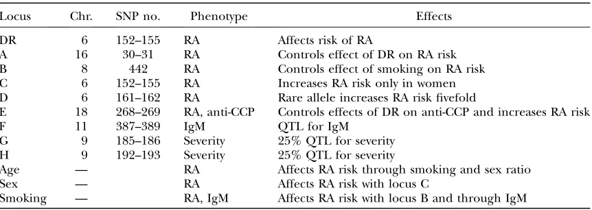
In Figure 3, the KWII (Figure 3A), TCI (Figure 3B), and PAI (Figure 3C) spectra, obtained using the PAI-based AMBIENCE search algorithm are compared to the corresponding results from an exhaustive search (EXS) of all combinations containing four variables or less for case study 1A. Figure 4, A–C, summarizes the spectra for case study 1B. The goal is to assess the effectiveness of the AMBIENCE search strategy by verifying that the critical interactions are identified.
For each method of search, the 20 combinations with the highest KWII values are presented each for one-variable, two-variable, and three-variable combinations. The spectra for four-variable combinations are uninformative and not shown for clarity. The solid bars in Figure 4, A–C, identify the peaks obtained by both the PAI-based AMBIENCE
Figure3.—A, B, and C are the KWII, TCI, and PAI spectra for case study 1A, respectively. All the one-variable-containing com-binations and the 20 two-variable and 20 three-variable comcom-binations with the highest KWII values are shown. The environmental variables are shown as E1, E2, E3, E4, the SNP variables are numbered 1–6, and phenotype is indicated as C. The combinations are indicated on they-axis. The error bars represent the standard deviations. The solid bars identify the peaks obtained by both the PAI-based AMBIENCE search algorithm and EXS methods, the open bars indicate the peaks obtained by the EXS alone, and the shaded bars indicate the peaks obtained by AMBIENCE alone.
search algorithm and the EXS methods, the open bars indicate the peaks obtained by EXS alone, and the shaded bars indicate the peaks obtained by AMBIENCE alone.
The KWII spectra in Figures 3A and 4A demonstrate that our PAI-based AMBIENCE search algorithm de-tects all peaks with significant GEI without the enumer-ation of all possible combinenumer-ations that is required in an exhaustive search approach. The KWII values of combi-nations containing only informative variables are un-affected by the LD between uninformative variables.
The patterns in the TCI and PAI spectra of case study 1A (Figure 3, B and C) are identical. The TCI spectrum of case study 1B (Figure 4B) shows prominent peak changes relative to Figure 3B for combinations {2, 3, 4, C}, {1, 3, 4, C}, {E4, 3, 4, C}, {E2, 3, 4, C}, {E1, 3, 4, C} and {3, 4, C} that are caused by the LD between the uninformative variables SNP 3 and SNP 4. These peak changes are absent in the PAI spectrum of case study 1B (Figure 4C), demonstrating that PAI is unaffected in the presence of LD between uninformative SNP variables. Thus the PAI is more effective than TCI in detecting GEI when LD between uninformative SNP variables is present.
The KWII spectrum (Figure 4A) shows that the AMBIENCE search algorithm correctly identifies the one-variable-containing peaks that demonstrate the crit-ical roles of E1, E2, SNP 1, and SNP 2 variables in the underlying model. A strong peak corresponding to the {1, 2, C} interaction is also identified. These peaks also feature in the KWII spectrum of EXS (as indicated by the shaded bars). None of the significant peaks in-volving an interaction between the known interacting variables are omitted in the spectrum of the PAI-based AMBIENCE search algorithm. All the peaks present in the KWII spectra of EXS only (open bars in Figures 3A and 4A) have very low magnitudes compared to the stronger peaks with known interactions. These results demonstrate that our search algorithm correctly identi-fies all known GEIs in both the case studies. Notably, the {E1, E2, C} combination was not present among the top 20 two-variable combinations with the highest KWII values in both the AMBIENCE search and EXS methods denoting the absence of any interaction between E1 and E2.
Case study 2:In case study 2, the GEI scheme (Figure
2B) consists of multiple environmental, biomarker, and
SNP variables whose interactions affect intermediate risk factors that contribute to the disease phenotype status. The schematic for the case study was motivated by the combinations of risk factors involved in congestive heart disease.
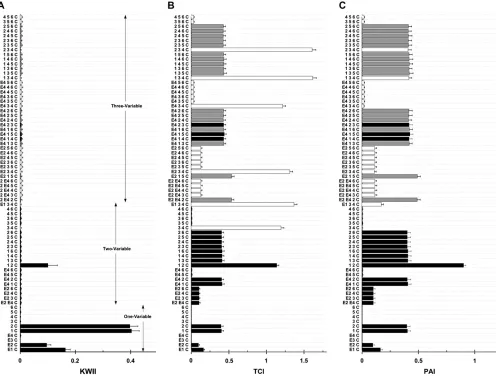
Figure 5, A, B, and C, summarizes the KWII, TCI, and PAI spectra, respectively, obtained using both the AMBIENCE algorithm and the EXS algorithm. For the KWII spectra (Figure 5A), combinations with the top 20 KWII values are presented each for one-variable, two-variable, and three-variable combinations.
The one-variable-containing peaks in the KWII spec-trum correctly detect the critical roles of E1, E2, B1, B2, SNP 1, SNP 2, and SNP 3 variables in the underlying model. Strong two-variable-containing interactions {E1, E2, C}, {E1, 1, C}, {B1, B2, C}, and {2, 3, C} were also identified. Again, all the peaks with significant KWII values that are detected by EXS are also identified by AMBIENCE. The KWII peaks that are detected by EXS alone (open bars in Figure 5A) are skipped during the
search process by AMBIENCE because these have very low magnitudes compared to the other stronger peaks present. The TCI and PAI spectra show that AMBIENCE identifies combinations with higher values of TCI (shaded bars in Figure 5B) and PAI (shaded bars in Figure 5C) than EXS (open bars in Figure 5, B and C), respectively. These results demonstrate that AMBIENCE correctly and efficiently identified all significant inter-actions in this relatively complex model.
We have analyzed a diverse range of additional case studies. In each case, AMBIENCE identified the key interacting variables effectively (data not shown).
Assessing robustness of PAI to LD: We critically assessed the variations in PAI values for different combi-nations in the presence of pairwise LD to evaluate the effectiveness of PAI for disease-associated GEI analysis.
We first examined the effect of LD between two SNPs that were not associated with the disease phenotype variable on TCI and PAI. We varied the LD between SNP 3 and SNP 4 from 0 to 1 for case study 1B in this
Figure5.—A, B, and C are the KWII, TCI, and PAI spectra for case study 2, respectively. All the one-variable-containing combi-nations and the 20 two-variable and 20 three-variable combicombi-nations with the highest KWII values are shown. The environmental variables are shown as E1, E2, E3, E4, the SNP variables are numbered 1–6, the biomarker variables are B1 and B2, and the phe-notype is indicated as C. The combinations are indicated on they-axis. The error bars represent the standard deviations.
experiment. The representative combinations {3, 4, C} and {E1, 3, 4, C} are presented because they include the two SNP variables in LD with each other (SNP 3 and SNP 4), the risk-increasing environmental variable E1, and the phenotype variable. The results (Figure 6A) dem-onstrate that as expected, the increasing LD between SNP 3 and SNP 4 contributes to the TCI of the com-binations containing these variables. In contrast to the TCI, which increases with increasing LD, the PAI remains unchanged: 0.00556SD 0.0027 in the absence of LD and 0.00436 0.0022 for LD¼0.9. Importantly for the {3, 4, C} combination the PAI remains at a value close to zero, indicating correct detection of no associ-ation between the SNPS and disease status despite the high LD. The TCI also correctly assessed no association between SNPs and phenotype in the absence of LD, 0.008660.0032; however, when LD between SNPs 3 and 4 was increased to 0.9, the TCI increased to a value of 1.196 0.037. In the second combination assessed, we include a risk-increasing environmental variable, E1, to {3, 4, C}. Because the {E1, 3, 4, C} combination contains the disease-associated E1 environmental variable, we correctly anticipated that both the PAI and the TCI values would be larger for {E1, 3, 4, C} than for {3, 4, C}. In the absence of LD, PAI and TCI were 0.17060.021 and TCI ¼0.178 6 0.021, respectively. When the LD between SNP 3 and SNP 4 was increased to 0.9, the TCI value combination increased.10-fold whereas the PAI was constant at 0.170 6 0.019. The PAI retained the disease association due to the presence of E1 while remaining unaffected by the LD between SNP 3 and SNP 4. Thus, in the presence of LD, PAI is a more effective metric than TCI for detecting disease pheno-type-associated GEI.
In the next set of experiments, we examined the effect of LD between two SNPs, one of which was associated with the disease phenotype variable. We modified case study 1A by introducing LD between SNP 3, which is not associated with the disease, and SNP 2, which is involved in the disease susceptibility. For this case (Figure 6B), the representative combinations {2, 3, C} and {E1, 2, 3,C} are presented. In the absence of LD, the TCI values of the {2, 3, C} and {E1, 2, 3, C} combinations were 0.4116 0.026 and 0.602 6 0.032,
respectively, and the PAI values were 0.40860.026 and 0.534 6 0.026, respectively. The higher TCI and PAI values in Figure 6B compared with 6A reflect the presence of informative variables in each of the combi-nations. In the presence of LD¼0.9, the TCI values of the {2, 3, C} and {E1, 2, 3, C} combinations increased to 1.49 6 0.046 and 1.68 6 0.048, respectively. The PAI values of the {2, 3, C} and {E1, 2, 3, C} combinations remained constant at 0.40060.029 and 0.53060.024, respectively at LD ¼ 0.9. Again, the results clearly indicate that the PAI effectively captured the genetic and environment risk-increasing information in the data while simultaneously filtering the spurious effects of LD in the {2, 3, C} and {E1, 2, 3, C} combinations.
In Figure 7, we investigate the relationship between TCI and a measure of LD,R2, as well as the sensitivity of
the PAI at varying levels of LD in real data for the Daly data set (Dalyet al. 2001). We computed PAI and TCI values for all two-SNP-containing combinations with the case–control status phenotype; the corresponding R2
values for these same SNPs were also computed to measure LD. The R2, TCI, and PAI spectra for 40
representative combinations varying in R2 values are
shown in Figure 7, A, B, and C, respectively. Compar-isons of Figure 7A to 7B demonstrate that the TCI spectrum mimics the dependencies present in the patterns of LD as measured by R2 values. Figure 7C
shows that in the presence of extensive pairwise LD, the TCI variations that closely resemble the LD patterns are not present in the PAI spectrum; consequently, PAI values are an order of magnitude (or more) smaller than the corresponding TCI values and the PAI spec-trum is relatively independent of the LD patterns.
These results indicate that the PAI is effective at detecting disease phenotype-associated GEI and is also robust to the confounding effects of complex patterns of dependencies among the genetic and environmental variables.
Performance of the PAI-based AMBIENCE algo-rithm on disease-relevant data sets: Performance on the
Daly data:To assess the performance of AMBIENCE, we
compared the results from the AMBIENCE analysis of the Daly data set (Dalyet al. 2001) to those obtained by
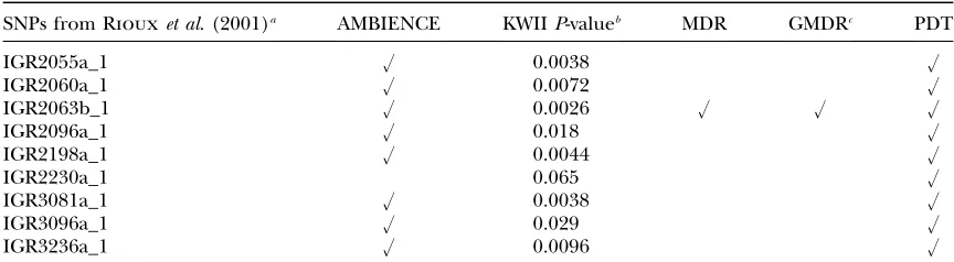
Riouxet al. (2001). Nine of the 11 SNPs on
some region 5q31 associated by Riouxet al. (2001) with the risk of Crohn’s were present in the data set we analyzed (see Table 2); SNPs IGR2078a_1 and IGR2277a_1 were missing (Chandaet al. 2007).
In the AMBIENCE analysis, 8 of the 9 reported SNPs (see Table 2) were present among the 20 combinations with the highest KWII values (spectra not shown). The permutation-basedP-values of the KWII for these SNPs (Table 2) ranged from 0.0028 to 0.029. We were unable to identify one SNP, IGR2230a_1 using AMBIENCE and it had a permutation-basedP-value of 0.065. Of the 103 SNPs present in the Daly data set, only 17 single SNP combinations had KWIIP-values#0.05 in permutation testing. AMBIENCE detected all 17 SNPs among the top 20 single SNP combinations with the highest KWII values.
10K GAW15 data set:The underlying GGIs and GEIs in
the simulations for this data set model the interaction of nine loci: C, DR, and D on chromosome 6, A on chromo-some 16, B on chromochromo-some 8, E on chromochromo-some 18, F on chromosome 11, and G and H on chromosome 9 (see Table 1 for a summary) (Milleret al. 2007). However, the anti-CCP and IgM measures are defined for the cases only. Although phase information was provided, we treated the data as genotype data for the AMBIENCE analysis.
The GAW15 data set contained 100 replicates from repetitions of the simulation procedure (Milleret al. 2007) and the availability of these replicates enabled us to compute the 95% confidence interval for the KWII of each combination.
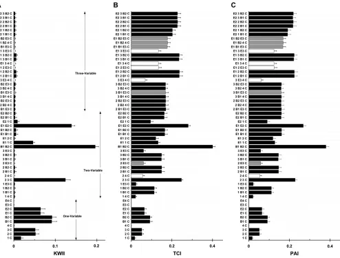
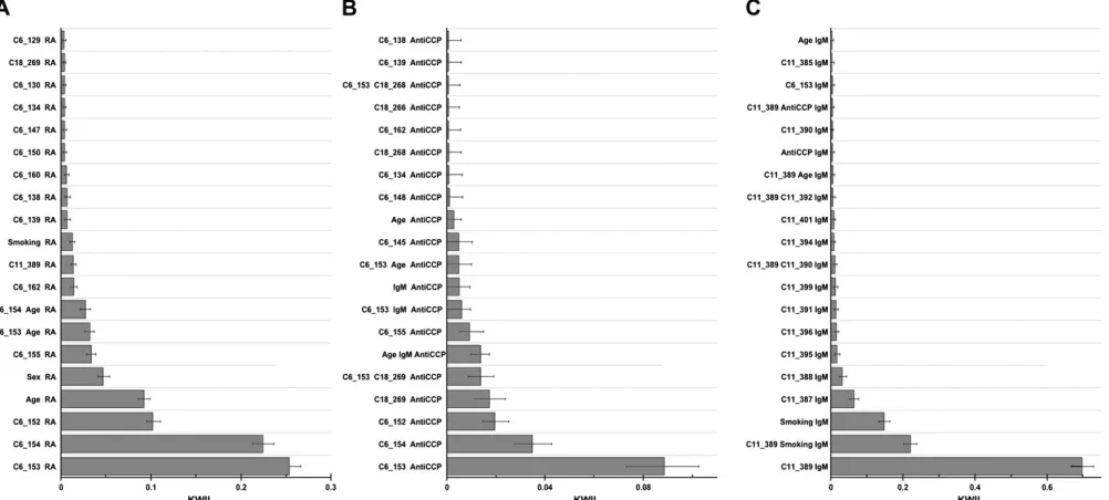
Figure 8 presents the KWII spectrum with RA affec-tion status as the phenotype. In interpreting the KWII
spectrum, a nonzero KWII value is significant and values greater than zero represent synergistic interactions. For example, in Figure 8A, we note that the KWII peaks for combinations {C6_153, RA}, {C6_154, RA}, {C6_152, RA}, {age, RA}, {sex, RA}, {C6_155, RA}, {C6_153, age, RA}, {C6_154, age, RA}, {C6_162, RA}, {C11_389, RA}, and {smoking, RA} are the combinations with the highest KWII values and also have 95% confidence intervals that do not include zero. These are therefore informative combinations in the KWII spectra. These combinations consist entirely of DR and locus C (both at SNPs C6_152-C6_155), locus D (C6_162), and locus F (C11_389) and the environmental variables age, sex, and smoking that had associations with the RA affection status in the simulated data set. Miller et al. (2007) built in pro-nounced effects of DR on RA affection status and this was confirmed by the highest values of KWII in Figure 8A that correspond to the DR locus. An interesting finding was the detection of the combination {C6_162, RA} corresponding to the locus D association with RA despite very low minor allele frequency (only 0.0083, making minor allele homozygotes very rare). Locus D has a direct effect on RA risk and each allele increases the hazard by fivefold (Milleret al. 2007).
Figure 8B presents the KWII spectrum with anti-CCP measure as the phenotype. The peaks with the highest KWII values (Figure 8B) enabled the identification of the following loci and covariates associated with the disease: loci C and DR (chromosome 6), locus E (chromosome 18), age, and IgM. The strongest con-tributions to the anti-CCP in simulations were from loci
Figure7.—TheR2(A), TCI (B), and PAI (C) spectra for 40 representative two-SNP-containing combinations with varying levels of LD as measured by theR2for the Daly data set (Dalyet al. 2001). The SNP combinations are indicated on they-axis.
E and DR; locus E affects anti-CCP by controlling which DR genotypes place a subject in the anti-CCP group with high mean values (Miller et al. 2007). Figure 8B demonstrates that the three highest KWII values corre-spond to the interaction between the DR locus (SNPs C6_152-C6_155) and the anti-CCP phenotype; the next two peaks, {C18_269, anti-CCP} and {C6_153, C18_269, anti-CCP}, correspond to the interactions of locus E alone and the locus E, DR combination with the anti-CCP phenotype.
Figure 8C presents the KWII spectrum with IgM as the phenotype. The peaks with the highest KWII values enabled the identification of the following loci and covariates associated with the IgM phenotype: loci C and DR (chromosome 6), locus E (chromosome 18), age, and smoking. When interpreting the KWII values of the {C11_389, IgM}, {C11_389, smoking, IgM}, and {smok-ing, IgM} combinations corresponding to the three largest peaks in Figure 8C, it is important to note that the KWII for each of these combinations does not contain redundant information;i.e., each of the combi-nations is significant on its own merit. Thus, the significant peaks for {C11_389, smoking, IgM} and {smoking, IgM} indicate that smoking alone is IgM associated but also contributes to the IgM phenotype synergistically in association C 11_389. Furthermore, the changes in the peak height should not be inter-preted to imply any protective role for smoking in the disease association.
Thus of the nine loci and three key covariates reported to be associated with the disease, we were able to identify five loci and all three covariates. We were unable to identify loci A, B, G, and H. Nonetheless, the performance of the KWII spectrum derived from AMBIENCE can be considered promising particularly given that AMBIENCE in its current form does not utilize either the haplotype–
phase information or the parent–child transmission in-formation contained in the pedigree structures.
Comparison to other competing approaches: We
compared our AMBIENCE approach to the MDR tech-nique (Ritchieet al. 2001, 2003; Hahnet al. 2003; Bush et al. 2006). All three methods were compared head-to-head on the SNP data set from Dalyet al. (2001) and the 100-SNP GAW15 data set.
Daly data set: The results from the head-to-head
comparisons of AMBIENCE to MDR, GMDR, and PDT on the Daly data set are summarized in Table 2.
The MDR method identifies {IGR2063b_1}, {IGR2063b_1, IGRX100a_1}, {IGR2063b_1, IGR2198a_1 IGR3066a_1}, and {IGR2063b_1, IGR2198a_1 IGR3066a_1, GENS0202ex3_2} as significant combina-tions associated with the Crohn’s disease phenotype. The MDR approach combination sets contained only two of the eight SNPs, IGR2063b_1 and IGR2198a_1, identified by Riouxet al. (2001) as being significantly associated with the Crohn’s disease phenotype. As expected, because the Dalyet al. (2001) data set lacked covariates, the GMDR results were identical to the corresponding MDR results. The PDT analysis, which was provided with the phase and family/transmission information in the Daly data set, identified all nine SNPs reported by Riouxet al. (2001).
100-SNP GAW15 data set: The results from the
head-to-head comparisons of AMBIENCE to MDR, GMDR, and PDT for the 100-SNP GAW15 data set are summa-rized in Table 3. The variables and the interactions identified by AMBIENCE have been previously dis-cussed in the sectionPerformance of the PAI-based
AMBI-ENCE algorithm on disease-relevant data sets and are also
summarized in Table 3.
The MDR analysis detected {C6_153}, {C6_154, age}, and {C6_153, age, sex} as associated with RA. The SNPs
TABLE 2
A comparison of the various competing methods to AMBIENCE using the Crohn’s disease-associated one-SNP combinations identified by RIOUXet al. (2001) as a reference
SNPs from Riouxet al. (2001)a AMBIENCE KWIIP-valueb MDR GMDRc PDT
IGR2055a_1 u 0.0038 u
IGR2060a_1 u 0.0072 u
IGR2063b_1 u 0.0026 u u u
IGR2096a_1 u 0.018 u
IGR2198a_1 u 0.0044 u
IGR2230a_1 0.065 u
IGR3081a_1 u 0.0038 u
IGR3096a_1 u 0.029 u
IGR3236a_1 u 0.0096 u
The SNPs that were correctly identified in a one-SNP combination by each method are shown with a check mark.
a
Two SNPs IGR2078a_1 and IGR2277a_1 were missing in our data set and are not included. b
TheP-values of KWII values were obtained by permuting case–control labels and assessing the proportion of KWII values of the permutations that exceeded the observed KWII.
c
C6_153 and C6_154 denote the chromosome loci C and DR, respectively. The MDR analysis did not detect locus D and E and smoking.
We analyzed the 100-SNP GAW15 data set using GMDR with sex, age, and smoking as the covariates and RA as the trait. The GMDR method identified the SNP combinations {C6_153}, {C6_153, C6_162}, {C6_153,
C6_154, C11_389}, where SNPs C6_153, C6_154 denote the chromosome 6 loci C and DR, respectively; C6_162 denotes locus D on chromosome 6; and C11_389 denotes locus F on chromosome 11.
We analyzed the 100-SNP GAW15 data set using the PDT as implemented in UNPHASED v3.10. Two derived data sets were used for analysis, one including only
Figure8.—The KWII spectra for one-variable- and two-variable-containing combinations for the ‘‘10K GAW15 data set’’ with rheumatoid arthritis (RA) affection status (A), anti-CCP antibody status (B), and IgM status (C) as the phenotype. The variable combinations are indicated on they-axis; the chromosome number and the SNP identifiers are provided for SNPs. The bars rep-resent mean values and the upper and lower error bars are the 95th and 5th percentiles of KWII values, respectively.
TABLE 3
A comparison of the various competing methods to AMBIENCE using the interactions used by MILLERet al.
(2007) in the GAW15 data set as a reference
Combination AMBIENCE MDR GMDR PDT
DR {DR, RA}, {DR, RA} {DR, age, RA}, {DR, age, RA},
{DR, age, RA} {DR, age, RA} {DR, sex, RA}, {DR, sex, RA}, {DR, age, sex, RA} {DR, smoking, RA} {DR, smoking, RA}
A, DR Not found Not found Not found Not found
B, smoking Not found Not found Not found Not found
C, sex {C, RA}, {C, RA} {C, sex, RA} {C, RA},
{Sex, RA} {C, age, sex, RA} {C, sex, RA},
{C, smoking, RA}
D {D, RA} Not found {C, D, age, RA}, {C, D, age, RA},
{DR, D, age, RA} {DR, D, age, RA}
E {E, RA} Not found Not found {E, RA, smoking}
Age, sex, smoking {Age, RA}, {DR, age, RA} a b
{Sex, RA}, {C, age, RA} {Smoking, RA}, {DR, age, sex, RA} {C, age, RA}, {C, age, sex, RA} {DR, age, RA}
a
GMDR requiresa prioricalculation of covariate effects, which are then incorporated into the analysis. Covariates cannot be analyzed alone. For ease of interpretation, we have used the same notation for results from all the methods.
b
PDT analyzes covariates simultaneously with genetic data; however, UNPHASED v3.10 is not designed to analyze covariates without genetic data.
nuclear families (6000 individuals) and one including all controls and one affected sibling selected at random from each family. Using both data sets we performed both single SNP analyses and analyses of all possible 2-SNP combinations with sex, age, and/or smoking status as effect modifiers of the trait RA. Both data sets identified the same loci as significant. After correction for multiple testing (Benjaminiand Hochberg1995) the PDT method identified loci DR, D, and E as associated with the RA phenotype and found locus C and sex as RA associated, specifically indicating an elevated risk of RA in women. As with the other methods, the PDT did not find locus A or B. Almost all of the false-positive associations were in regions contiguous with the true associations.
Time complexity and computational speed: The
AMBIENCE search algorithm is computationally much more efficient than exhaustive search, which requires computing all possible combinations and requires exponential time.
Here, we borrow the notation from complexity theory (Corman et al. 2001) to assess the computational complexity of the AMBIENCE algorithm. Letmbe the sample size of the data andnbe the number of variables (excluding the phenotype variable). Lines 2–5 take O(n 3m2) computations because of PAI computation
that consumesO(m2) computations and lines 6 and 16
takeO(u3n) computations each. Lines 7–15 takeO(t3
n3u3m2) computations since PAI computations are
re-peated fort(forloop in line 7)3n(forloop in line 9)3u (forloop in line 10) computations. Finally, lines 17–22 takeO(t3u 32t3
m2) time since KWII needs to be
computed for all possible subsets for a maximum com-bination size oftfor each ofucombinations that were obtained at each step oftiterations. However, in genetic applications, the range of t-values of interest is small because of sample size constraints, which limits the computational complexity from becoming exponen-tially large.
The AMBIENCE algorithm was used to search for combinations containing up to three variables withu¼ 50 using the computational speed GAW15 data sets as the test bed. The computations were conducted on a Hewlett-Packard Proliant server with four dual-core
2.8-GHz processors with 16 GB of memory and running the Linux operating system.
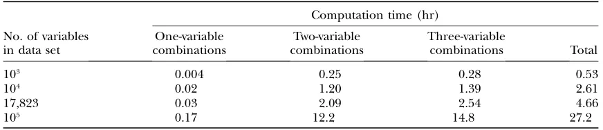
Table 4 summarizes the total time requirements and the time requirements for one-variable-, two-variable-, and three-variable-containing combinations. These re-sults indicate that increasing the size of the combina-tions has only a modest effect on the computation time of AMBIENCE.
DISCUSSION
In our information theoretical framework, which is novel for GEI analysis, combinations with positive values of KWII are operationally defined as interactions. In this report, we developed and evaluated the PAI, a TCI-based information theoretic metric, to enable compu-tationally efficient searching of the GEI combinatorial space. The PAI is more robust than the TCI when interdependencies among multiple variables such as those caused by LD are present. We also critically evaluated the effectiveness and computational effi-ciency of the PAI-based AMBIENCE search algorithm for GEI analysis. Our results demonstrate that these methods are effective for analyzing a diverse range of epidemiologic data sets containing complex combina-tions of direct effects and multiple GEI.
The information theoretic AMBIENCE approach is flexible and can be used when the genetic and environ-mental variables have different numbers of classes or when the phenotype has more than two classes. This means that SNP and microsatellite markers can be analyzed together if necessary. Another critical advan-tage with our approach is that it provides options for user interactions and visualization for small data sets. For example, the incremental effect of adding a SNP can be easily visualized on the PAI spectrum. The ability to interact with data enriches the user’s experience and can enable detection of features that are otherwise difficult to find. In addition to its information theoretic underpinnings, which are novel for GEI analysis, a key difference between AMBIENCE and other methods such as MDR and GMDR is that the AMBIENCE approach uses a greedy search algorithm based on the PAI rather than dimensionality reduction. However,
TABLE 4
Computational speed for the AMBIENCE algorithm
Computation time (hr)
No. of variables in data set
One-variable combinations
Two-variable combinations
Three-variable
combinations Total
103 0.004 0.25 0.28 0.53
104 0.02 1.20 1.39 2.61
17,823 0.03 2.09 2.54 4.66
AMBIENCE may be compatible with dimensionality reduction methods. It is also noteworthy that the in-formation theoretic metrics in AMBIENCE are sensitive to both linear and nonlinear dependencies in the data.
At first sight, our KWII-based definition of interaction would appear to differ from the more conventional definition of interactions in statistical genetics. Statisti-cal interactions represent deviations from additivity that are present in data: they are said to occur when the probability of observing the phenotype states for a variable combination is greater (or less) than expected from the probabilities of the phenotype states for each of variable considered individually. Count data are commonly analyzed using logistic regression and in this framework, interactions are assumed to be present if the parameters for the product terms are significant. We have conducted simulations with a diverse range of models, many of which could not be included in this article in the interests of brevity, that indicate a remark-able degree of concordance between the GEIs identi-fied by our method and those identiidenti-fied by other methods. Specifically, we have also conducted a KWII-based analysis of the two-locus interaction models of pure epistasis analyzed by Culverhouse(2007). These models are defined by penetrance matrices and result in two-locus interactions that are devoid of any main effects. We found (results not shown) that the KWII spectra successfully found the combination of the two variables involved in the interaction and did not contain peaks from any of the uninformative variables or combinations. The qualitative concordance of the KWII with the challenging models used by Culverhouse (2007) and its performance in the case studies further demonstrate the utility of the KWII-based definition for GEI applications and data sets is reassuring and repre-sent an important step for our novel approach.
Although the KWII is effective at identifying two-locus interaction models of pure epistasis (Culverhouse 2007), AMBIENCE is likely to have less power than MDR at identifying informative combinations in such pure epistasis examples because it utilizes a marginal effect strategy. The Boolean XOR gate ( Jakulin and Bratko2003) is another example of a pure interaction that would be difficult to identify with AMBIENCE. Nonetheless, a pure epistasis interaction has stringent symmetry requirements that are rarely met in real data; this can be readily observed, e.g., in synthetic and symmetric appearance of the penetrance matrices employed by Culverhouse(2007). In real data, small differences in allele frequency cause traces of lower-order effects that can be detected by AMBIENCE. This weakness in AMBIENCE can be readily addressed by conducting an extensive search of two-variable combi-nations. However, in data sets with large numbers of genetic and environmental variables, MDR-based meth-ods can also suffer from loss of power because the number of variables that can be analyzed is limited and
users may not be able to identify the key variables for inclusion. Thus, MDR-based methods and AMBIENCE can suffer from loss of power under certain circum-stances but for different reasons.
Although the KWII is very effective at detecting GEI, its correspondence with logistic regression is not exact ( Jakulin 2005). The lack of exact correspondence is attributable in part to methodological differences: logistic models fit all the terms simultaneously to the data, whereas with the KWII approach, higher-order interactions are inferred after eliminating lower-order contributions.
The AMBIENCE algorithm was found capable of identifying the strongest interactions containing #3 variables in the 100,000 SNP-containing computational speed GAW15 data set with 27 hr of computational time. However, our goal is to extend the method so that it is capable of conducting 106- to 107-variable analyses
and match the data acquisition capabilities of the Affymetrix and Illumina genotyping platforms. This goal should be considered feasible particularly given improvements,e.g., parallelization that can be used to boost the performance of the AMBIENCE algorithm.
Both MDR and AMBIENCE require the user to specify the maximum combination order, which is the principal determinant of computational load. However, methods based on MDR are computationally intensive because they conduct an exhaustive search of both the genotype and the variable spaces. AMBIENCE is focused on identifying interacting variables and derives its compu-tational efficiency because it conducts a directed search that harnesses the PAI via a greedy search algorithm. The monotonic properties of the PAI assist in highlight-ing combinations with high KWII values.
To minimize estimation errors resulting from the limited cell counts for higher-order combinations, MDR conducts cross-validation of the multilocus genotypes in each variable combination. Although AMBIENCE currently implements a permutation-based P-value as-sessment after identifying the set of promising combi-nations, the inclusion of a permutation test within each stage can be expected to further improve its perfor-mance. Despite these weaknesses and differences vis-a`-visother methods, AMBIENCE has capabilities that are not present in any of the existing methods;e.g., it can handle data sets with three or more outcomes.
Nonetheless, the available GEI methods such as MDR, GMDR, and PDT that employ dimensionality reduction do different things and ask different questions. For example, PDT is a method that is particularly useful for family-based study designs and can accommodate miss-ing data whereas MDR is a nonparametric dimension-ality reduction method for case–control study designs. The GMDR method is capable of handling continuous covariates. To ensure a fair comparison of the compet-ing methods, despite their underlycompet-ing differences, we provided each competing method with relevant data