LEVY, RACHEL. Partial Differential Equations of Thin Liquid Films: Analysis and
Numerical Simulation. (Under the direction of Michael Shearer.)
We consider four problems related to Marangoni-driven thin liquid films. The first
compares two models for the motion of a contact line, the triple point at which solid,
liquid and air meet, which is a major outstanding problem in the fluid mechanics
of thin films. The precursor model replaces the contact line by a sharp transition between the bulk fluid and a thin layer of fluid, effectively pre-wetting the solid; the
Navier slip model replaces the usual no-slip boundary condition by a singular slip condition that is effective only very near the contact line. We restrict attention to
traveling wave solutions of the thin film PDE for a film driven up an inclined planar
solid surface by a thermally induced surface tension gradient. This involves
analyz-ing third order ODE that depend on several parameters. We find that the range
of effective contact slopes in both models is confined to an interval bounded away
from zero. Moreover, the precursor model breaks down in an unexpected way as the
precur-even when both heights are equilibria of the ODE. This is explained with the aid of
Poincar´e sections of the phase diagram of the ODE. In the second problem, we apply
a theory of scalar conservation laws that includes a kinetic relation and nucleation
condition, to our model for the flow of thin liquid films. As in the previous problem,
the context is the flow of a thin liquid film up an inclined planar solid substrate, the
flow being driven by a surface tension gradient against the action of gravity. Our
goal is to use theory from hyperbolic conservation laws to map the rich set of wave
structures that arise as solutions to the Cauchy problem, including classical shocks,
nonclassical shock waves (known as undercompressive shocks) and rarefactions. To
create such a ’Riemann map’, we employ a kinetic relation that describes admissible
nonclassical shock waves, and a nucleation condition that determines when a
nonclas-sical solution is selected. The hyperbolic theory is able to capture features observed
in thin film flow, such as multiple long-time solutions for the same initial upstream
and downstream states. The third problem incorporates localized heating by an
infrared (IR) laser to the model of a Marangoni-driven thin film from the previous
problems. We analyze two types of steady state solutions, using a dynamical systems
approach to explain homoclinic solutions and PDE simulations to explain heteroclinic
solutions. The Riemann map developed in the previous problem predicts the effect of
initial conditions on the development of wave structures. We discuss several methods
explores a model for a different physical scenario, in which a thin film is driven down
a solid substrate by gravity and surfactant, surface-active-agent that lower surface tension. The problem is motivated by application of surfactants in medicine to
im-prove lung function in premature infants by lowering surface tension in the alveoli.
The model couples the thin film PDE for the height of the film with an equation for
the transport of surfactant. Solutions of the parabolic-hyperbolic system include a
complicated double wave solution, with discontinuities in the height and surfactant concentration gradient. We explain the solutions analytically using two types of
dis-continuous solutions and traveling waves. Agreement of the analytical solutions with
data from numerical simulations indicates that we have successfully modeled
long-time wave structures, including a linear increase in the maximum of the surfactant
THIN LIQUID FILMS: ANALYSIS AND
NUMERICAL SIMULATION
by
Rachel Levy
a dissertation submitted to the graduate faculty of
north carolina state university
in partial fulfillment of the
requirements for the degree of
doctor of philosophy
applied mathematics
raleigh, north carolina
April 2005
approved by:
M. Shearer
chair of advisory committee
A. Chertock
Rachel Levy was born in Wilmington, North Carolina. She graduated from the
North Carolina School of Science and Mathematics and went on to study English and
Mathematics at Oberlin College. She has a Master of Arts in Educational Media and
Instructional Design from the University of North Carolina at Chapel Hill. In addition
to teaching middle and high school at Carolina Friends School in Durham, North
Carolina, she served one year as Upper School Dean. Rachel taught mathematics at
the Duke University Talent Identification Program, edited Mathegraphics magazine
and served as supervisor of the Mathematics Summer Program.
At North Carolina State University, Rachel completed the requirements for
certi-fication in Computational Science and was awarded a fellowship from the Center for
Research in Scientific Computing. She was also selected for two teaching fellowships:
the Future Professors Pilot Program at Microsoft and and Preparing the Professoriate
Program at North Carolina State University. At the British Applied Mathematics
Colloquium she received a prize for Best Student Talk.
Rachel is a member of SIAM, AWM, AMS and Pi Mu Epsilon. At North Carolina
Association and of the SIAM Student Chapter.
I would like to thank my advisor, Michael Shearer for his patience, encouragement
and support. His love of mathematics and research is truly contagious. I would also
like to thank the other members of my committee, Alina Chertock, Mette Olufsen
and Tom Witelksi. For their encouragement throughout graduate school I would
like to thank Karen Daniels, Andrea Bertozzi, Greg Forest, and Robert Behringer.
Thank you to the N.C. State Mathematics Department for providing a supportive
atmosphere for research, teaching and learning.
Over the past four years the physicists, engineers and mathematicians of the
focused research group in thin films and fluid interfaces have greatly enriched my
interest in research.
Jill Reese, Brian Adams, and Iti Janovitz have made life in Harrelson Hall
es-pecially pleasant. Ryan Haskett shared the localized forcing problem with me and
Barry Edmonstone shared the surfactant problem with me. Randall Nortman
pro-vided expert advice on computing.
Thank you to my parents, brother and extended family for encouraging me in
who have cheered me on. Love and gratitude to my beloved Sam, Tulani and Miryam,
who never wavered in their support of me and this work.
This research has been supported by NSF Grants DMS-9803305, DMS-0244491
and the Department of Mathematics and Center for Research in Scientific
Computa-tion, North Carolina State University Raleigh, NC 27695.
List of Tables xi
List of Figures xii
1 Introduction 1
1.1 Introduction to thin liquid films . . . 3
1.2 Pioneering work in fluid dynamics . . . 5
2 The Thin Film Experiment 11 2.1 Description of the Physical Experiment . . . 11
2.2 Derivation of the Scalar Thin Film Equation . . . 17
2.2.1 Velocity of the Flow and Gravity . . . 17
2.2.2 Navier-Stokes Equations . . . 18
2.2.3 The Lubrication Approximation . . . 19
2.2.4 Boundary Conditions . . . 21
2.2.5 Integrating the PDEs . . . 24
2.2.7 Conservation of Mass . . . 26
2.2.8 Non-dimensionalization . . . 27
3 Comparison of Contact Line Models 29 3.1 Introduction . . . 29
3.2 The ODE Models . . . 32
3.2.1 The Navier Slip Model . . . 32
3.2.2 The Precursor Model . . . 33
3.2.3 Comparison . . . 34
3.2.4 Equilibria . . . 35
3.2.5 Parameter Ranges for Equilibria . . . 40
3.3 Numerical Experiments . . . 43
3.3.1 Phase Portraits and the Poincar´e Section . . . 44
3.3.2 Contact Slopes . . . 46
3.4 Discussion . . . 54
4 Kinetics, Nucleation and the Riemann Solver 56 4.1 Introduction . . . 56
4.2 Background on Kinetics and Nucleation . . . 58
4.3 Hyperbolic Theory . . . 61
4.4 Traveling Waves . . . 75
4.5.1 ODE Numerical Solutions . . . 86
4.5.2 PDE Numerical Solutions . . . 92
4.6 Finite Difference Scheme for Thin Film Equation . . . 102
4.6.1 Boundary Conditions and Initial Data . . . 103
4.6.2 Newton’s method . . . 104
4.7 Discussion . . . 105
5 Thin Film Experiment with Localized Heating 106 5.1 Experimental Setup and Mathematical Model . . . 106
5.2 Analysis of Type I Solutions . . . 109
5.3 Analysis of Type II Solutions . . . 117
5.3.1 Interpretation of Type II wave structures using the flux plot . 122 5.4 Discussion . . . 124
6 Surfactant-Driven Thin Film Flow 126 6.1 Introduction . . . 126
6.2 The Model . . . 130
6.3 Smooth Traveling Waves . . . 133
6.4 Discontinuities and the Rankine-Hugoniot Condition . . . 136
6.5 Symmetries . . . 139
6.6 The Horizontal Substrate: α = 0 . . . 143
6.6.2 Discontinuous Solutions for α= 0, D= 0 and Γ >0. . . 144
6.6.3 Discontinuous Solutions for α= 0, D >0 with Γ = 0. . . 150
6.6.4 Discontinuous Solutions for α= 0, D >0 with Γ >0. . . 151
6.6.5 Nonlinear Traveling Waves forα = 0, D = 0 . . . 152
6.7 The Inclined Substrate: α >0, D = 0.. . . 153
6.7.1 Discontinuous Solutions for α >0, D = 0,Γ = 0 . . . 154¯
6.7.2 Discontinuous Solutions for α >0,D= 0, ¯Γ>0 . . . 156
6.7.3 Smooth Traveling Wave Solutions . . . 161
6.8 Numerical Simulations . . . 164
6.8.1 Composite Finite Difference Scheme . . . 165
6.8.2 Initial Conditions . . . 167
6.8.3 Numerical Simulations Exploring Simple Jumps, α = 1, D= 0 169 6.8.4 Structure of Solutions for α= 1, hL = 1, hhRL < √ 3−1 2 . . . 170
6.8.5 Structure of Solutions for α= 1, hL = 1, hhRL > √ 3−1 2 . . . 171
6.8.6 Numerical Simulations, α= 0 . . . 172
6.8.7 Oscillations with Crank-Nicolson, α >0 . . . 172
6.8.8 Distinguishing Shocks from Steep Gradients . . . 174
6.9 Analysis of Double Jump Solution . . . 174
6.9.1 The Double Jump Solution: Traveling Waves and Simple Jumps 175
simple Jumps . . . 178
6.9.3 Use of Maple to calculate parameter values for a semi-simple
jump . . . 179
6.10 Discussion . . . 182
References 191
3.1 Model Specifications . . . 35
3.1 Parameter Specifications . . . 44
4.1 Relationship between jump-up/down cases, orbits, and types of wave. 90 6.1 Types of jumps for different parameter spaces . . . 137
6.2 Roots ofd(h) leading to asymptotes for Γ(h). . . 163
6.3 Analytical and numerical results for semi-simple jump . . . 181
6.4 Calculated values of corrections for semi-simple jump . . . 182
2.1 Schematic of thin film experiment. . . 12
2.2 Illustration of experiment and film profile. . . 12
2.3 Photographs of thin film experiment. . . 14
2.4 Components of gravity in the thin film problem. . . 18
3.1 Flux functions. . . 36
3.2 Choosing initial data on the invariant manifold. . . 39
3.1 Macroscopic View of Poincar´e section. . . 46
3.2 Poincar´e sections for the precursor model. . . 47
3.3 Effect ofδ on precursor length. . . 47
3.4 Single trajectories. . . 48
3.5 Navier slip model: Single Trajectories. . . 49
3.6 Effective contact slope for precursor model when hm = 0.30. . . 50
3.7 Range of contact slopes for Navier slip model, β = 0.013, hm = 0.26. . 51
3.8 Effective contact slope vs. actual contact slope. . . 52
0.037. . . 54
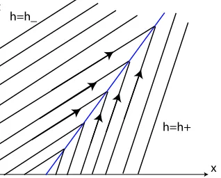
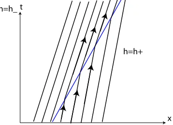
4.1 Illustration of classical shock fromh to h+ . . . 63
4.2 Illustration of nonclassical shock fromh toh+ . . . 64
4.3 Illustration of rarefaction from h toh+ . . . 69
4.4 Illustration of admissible rarefactions . . . 70
4.5 Numerical simulation of classical and non-classical shock waves. . . . 72
4.6 Plot of the flux function. . . 74
4.7 Illustration of three equilibria, intersections between a chord and the flux plotf(h) =h2−h3 . . . . 77
4.8 Plot of h versus G(h) for an undercompressive wave connecting h1 = 0.558 to hb = 0.1. . . 80
4.9 Plot ofh versus G(h) for a reverse undercompressive wave connecting hb = 0.1 to h2 = 0.7287. . . 81
4.10 Plot of h versus G(h) for a wave connecting hb = 0.1 to h∗ = 0.665. . 81
4.11 Kinetic relation for undercompressive shocks (left) and for reverse un-dercompressive shocks (right). . . 84
4.12 Nucleation Condition: Jump-down case (left); jump-up case (right). . 85
4.13 Poincar´e Sections: Jump-down case. . . 88
4.14 Poincar´e Sections: Jump-up case. . . 89
compressive shock; R: rarefaction wave. . . 90
4.16 Solution of the Riemann Problem. C: classical shock, U: undercom-pressive shock; R: rarefaction wave. . . 92
4.17 Solution of the Riemann Problem for fixed hR <1/3 . . . 93
4.18 Riemann Problem Solutions for fixed hL . . . 99
4.19 Non-monotonic initial data: jump-down and jump-up cases. . . 100
4.20 Non-monotonic initial data: narrow versus wide ridge. . . 100
4.21 Tracking waves in the flux function. . . 101
4.22 Transients and wave interactions preventing nucleation. . . 101
5.1 Experimental setup with localized forcing. . . 107
5.2 Profiles of type I steady state solutions. . . 110
5.3 Multiple type I solutions . . . 112
5.4 M versus maximum and minimum values of h . . . 113
5.5 Schematic of manifolds for small M. . . 116
5.6 Bifurcation diagram with type IIMc. . . 118
5.7 Evolution of type II state from horizontal h0. . . 119
5.8 Upstream and downstream heights for type II steady state solutions. 120 5.9 Nucleation of double wave structure. . . 121
5.10 Film evolution and corresponding waves on flux plot. . . 122
6.1 Alveoli with and without surfactant. . . 127
6.3 Dynamics on Γ(h) for α= 0. . . 153
6.4 Effect of speeds on maximum of Γ. . . 159
6.5 Dynamics on Γ(h) for α= 1. . . 164
6.6 Traveling wave plot, α= 1. . . 165
6.7 Plots illustrating a variety of initial conditions. . . 183
6.8 Numerical simulations of simple jumps forα= 1. . . 184
6.9 Typical solution profile with labels for important parameters. . . 185
6.10 Numerical simulations varying downstream height hR. . . 186
6.11 Wave development for hL=hR= ΓL= ΓR= 1. . . 187
6.12 Numerical simulations, α= 0. . . 187
6.13 Phase portrait of Γ versus h for α= 0. . . 188
6.14 Oscillations in numerical results from Crank Nicolson method. . . 188
6.15 Grid refinement to illustrate shock. . . 189
6.16 Evolution of h and Γ . . . 189
6.17 Phase portrait of Γ versus h for α= 1. . . 190
Introduction
The story of the research of thin liquid films is one of successful collaborations between
mathematicians, physicists and engineers. It begins with the general study of fluid
dynamics in which scientists modeled observable macroscopic events, and leads to the
recent study of microfluidics, in which even the most advanced imaging techniques
do not answer fundamental questions about the motion of fluids.
This thesis focuses on ODE and PDE models of thin liquid films driven by
Marangoni forces. Marangoni forces, named after Carlo Marangoni (1840-1925), are
induced by surface tension gradients. These forces are able to drive liquids from one
area to another because the liquids are drawn to regions of higher surface tension. We
will consider two mechanisms for inducing Marangoni forces: heat and surfactant.
The first five chapters of the thesis will focus on a physical experiment in which
a thin film is driven up an inclined solid substrate by a heat-induced surface tension
gradient. As discussed in Chapter 2, the experiment is modeled by the Navier-Stokes
equations and the lubrication approximation.
Chapter 3 contains new results comparing two models for the contact line of a thin
film: the Navier slip model and the precursor model. The modeling of the motion
of a contact line, the triple point at which solid, liquid and air meet, is a major
outstanding problem in the fluid mechanics of thin films [5, 18]. We consider an ODE
model based on traveling wave solutions of the PDE to compare admissible parameter
ranges and contact slopes. For this model we present both analytical and numerical
results.
Chapter 4 contains a new Riemann solver for the precursor model. The solver
employs a nucleation condition and kinetic relation proposed by LeFloch and Shearer
and theory from hyperbolic conservation laws to predict the development of wave
structures in solutions of the hyperbolic PDE. Again we present both analytical and
numerical results. Using a one-dimensional model, we will explain classical and
non-classical wave structures that develop in thin liquid films.
Chapter 5 adds localized Marangoni forcing to the thin film experiment. Two
distinct steady state solution profiles form, and we connect information from the
Riemann solver to the development of these solutions.
Chapter 6 explores a different physical scenario in which a thin film runs down a
substrate and is additionally driven by a surfactant-induced Marangoni force. The
type. One equation is for the height of the thin film, the other is for the surfactant
concentration. The solutions of the PDE contain jumps in height and surfactant
concentration gradient. For this problem we use theory adapted from hyperbolic
conservation laws to explain long time solutions.
1.1
Introduction to thin liquid films
Thin liquid films coat surfaces, such as computer chips, with layers as thin as
thou-sandths of a millimeter. Ideally the film would have a perfectly uniform height. In
reality, thin films are uneven, both in height where capillary effects and wave
struc-tures cause bumps in the film, and at the contact line, where fingering instabilities
(such as drips of paint) [12, 21, 69] and precursor layers may develop. Precursor layers
can be a uniform film that prewets the entire surface or a layer of fluid at the leading
edge of the film that wets the surface before the bulk of the fluid follows. In order
to understand, predict and control the behavior of thin films, we study how the films
develop, what governs their height and what conditions produce a flat, even film.
There are two primary types of thin films, solid films that are created by vacuum
vapor deposition and liquid films that are created by driving a coating layer of liquid
onto a surface by means of an external force, such as gravity, surface tension or
centripetal force (as in spin coating of computer chips). We are interested only in the
second type: driven thin liquid films.
that supplies the liquid. This is sometimes called the upstream region, and the
profile of the film as it emerges from the reservoir is referred to as the meniscus. Far downstream, at the leading edge of the film where air, liquid and solid substrate meet,
is the contact line. The geometry and mechanism for movement of the contact line are unresolved subjects to this day [62, 53, 56]. The contact line can become unstable
and develop fingering instabilities. To eliminate contact lines in experiments, the substrates are prewetted with a monolayer of the film fluid, to form a prewetting
layer called a precursor layer. Behind the contact line, a common feature of thin films is a capillary ridge, a bulge of fluid behind the contact line that builds up faster than the film can spread on the surface.
Important properties of the fluid include the viscosity, temperature, density, and
pressure. These properties are an important consideration when choosing fluids for
experimental purposes. Silicone oils are commonly used in thin film experiments
because they are chemically inert to most materials (including rubber, plastic and
metals), and thermally stable, even when heated or cooled for long periods of time.
Silicon wafers are used as a substrate, perhaps inspired by applications in the
com-puter chip manufacturing industry. Before the rise of the comcom-puter industry, other
liquids and substrates, such as honey on glass or olive oil on silver plate were used by
1.2
Pioneering work in fluid dynamics
The models for thin films, like those for many fluid flow phenomena, are based on
the Navier-Stokes equations, a system of non-linear partial differential equations
de-veloped by Claude-Louis Navier (1785-1836) and George Gabriel Stokes (1819-1903)
to describe the flow of fluids such as liquids and gases. The equations, expressing
conservation of mass and momentum, are used to model a wide array of fluid flow
phenomena, such as the movement of air in the atmosphere, ocean currents, and
wa-ter flow in a pipe. While there has been extensive research into the Navier-Stokes
equations, there are unresolved mathematical issues, including existence and
smooth-ness, which are the subject of one of the famous Millennium Prize Problems, posed
by the Clay Mathematics Institute in May, 2000.
Fluid mechanics and associated phenomena have probably been observed as long
as people have been around water and air. With the rise of empirical science and
mathematics, the general scientific study of fluid mechanics continued to receive
at-tention. The study of thin liquid films dates back to observations of oil slicks on
water, which led to conjectures about monomolecular layers and calculations of the
size of molecules by Franklin [24], Pockels [57] and Rayleigh [57].
More recently, the computer chip industry and improved imaging techniques have
advanced the study of thin liquid films. Computer chip manufacturers want thin,
even coating layers, and have supported research efforts to create even films.
their properties. Both industrial needs and technological advances prompted research
in surface chemistry, with significant advances in the 1970’s.
The mathematical interest in thin liquid films combines the Navier-Stokes
equa-tions with new ideas. In the 1970’s, several papers were published that combined two
critical ideas. The first was the already well-known [34] lubrication approximation,
which took advantage of the thinness of the film through the small quantity
= H
L (1.1)
in which H is the characteristic height of the film and L is a characteristic length
such as the length of the substrate. When applied to the Navier-Stokes equations,
the equations can be simplified by retaining the terms in each equation that contain
the lowest power of .
The second idea was to resolve the stress singularity at the moving contact line
of the film, the triple point at which gas, liquid and solid meet. This required a
rethinking of the commonly accepted no-slip boundary condition between liquid and
solid, which could not account for the movement of the contact line.
Ludviksson and Lightfoot (1971) published an experimental and theoretical
inves-tigation of Marangoni films climbing up vertical solid surfaces. They confirmed that
derived a hydrodynamic model leading to the equation
ht =
∂ ∂z
1
µ
∂p ∂z +ρg
h3 3 −
γh2 2µ
(1.2)
to describe film growth, but acknowledged a problem with this model for no slip at the
contact line, since ht = 0 when h= 0. They suggested that the edge of the meniscus
advances by a “diffusional process which is most probably made possible by
multi-layer adsorption in a very thin primary film formed ahead of the meniscus”, that is,
a precursor film. They cite several instances of observations of such a film, and note
finite contact angles at the contact line in their experiments. In their experiments,
they used squalene for the liquid and a polished silver plate for the substrate.
Huh and Scriven (1971) published a paper containing a hydrodynamic model of
the contact line, based on the observation that perfect slip can only be applied if the
dynamic contact angle at the contact line is zero. They note that “shear stresses,
pressure and viscous dissipation rate increase without bound as the contact line is
approached.” They catalog static and dynamic contact angles, and compare them
to observed experimental results. They discuss options for kinematic and dynamic
boundary conditions, allowing for slip at the solid surface, and in some cases including
intermolecular forces. However, the continuity of the stress tensor across the
fluid-fluid interface (in a two-fluid-fluid system) is not satisfied and the velocity field implies the
fluid exerts an infinite force on the surface of the fluid at the contact line.
through a series of qualitative experiments. They conclude that “the no-slip boundary
condition and the moving [contact] line are kinematically incompatible concepts.”
They use honey on glass, and glycerin on beeswax to illustrate their points. They
also use a combination of glycerin, silicone oil, food dye and plexiglass, to illustrate
a rolling motion of the fluid.
In 1976, Dussan continued her analysis of the moving contact line problem with a
further discussion of the slip condition. She notes that in 1965, Goldstein suggested
a linear boundary condition ¯β(U −1), where ¯β is called the slip constant. He also pointed to papers by Navier in the 1800’s that mentioned the concept of a no slip
boundary condition. Dussan claims that the differences between several slip models
can only be observed on a length scale less than a micrometer.
Also in the 1970’s, Hocking wrote several theoretical papers about the movement
of fluids on different surfaces and the removal of the force singularity at the contact
line through the use of a slip boundary condition, which he called a ‘slip flow’. [31, 32].
Greenspan (1978) studied the motion of a thin viscous droplet wetting a surface.
His model included the lubrication approximation and a dynamic contact angle. He
notes that at the time, hydrodynamics on the micro-scale was a largely unexplored
area. Greenspan cites experimental evidence of a precursor layer only Angstroms
thick in the work of Ghiradella and Radigan (1975) and in the work of Schwartz
and Tejada (1972). Greenspan assumes that “the theoretical dynamic contact angle
chooses a slip condition of the form
κ(h)uz =u, κ(h) =
α
3h, α=O(10
−10cm2) (1.3)
at the boundary z = 0.
By the mid 1980’s, the question of appropriate boundary conditions for thin film
flow was unresolved, but many theories about the physics at a microscopic level had
evolved. Many of these are cataloged in the 1985 paper by deGennes [18]. One
devel-opment was the inclusion of van der Waals forces in the models, which is discussed
at length in a book by Israelachvili [36].
By the early 1990’s DeGennes was collaborating with Cazabat and colleagues
on incompressible flows, including spreading of droplets [19]. Our story begins in the
1990s, when Cazabat and her colleagues at the College de France in Paris designed an
experiment to investigate thin films of silicone oil coating a silicon wafer. Surprising
experimental results led to the discovery of non-classical waves in thin liquid films,
which are the subject of Chapters 2, 3, 4 and 5 of this thesis. Chapter 6 contains
analysis and numerical simulations modeling a thin film driven down an inclined
plane by gravity and surfactants, chemical agents that reduce surface tension. The
connection to previous chapters is that the model is a system of equations, the first
of which is a thin film PDE for the height of the film. This equation is coupled
to a second PDE for the surfactant concentration on the surface of the film. We
solutions developed in earlier chapters as well as new approaches. An introduction to
The Thin Film Experiment
2.1
Description of the Physical Experiment
In the 1990’s, Anne Marie Cazabat and her group at the College de France in Paris
conducted experiments with thin liquid films of PDMS (PolyDiMethylSiloxane) oil
coating silicon wafers [12, 23]. We describe the experiment as it was later replicated
and extended by Robert Behringer and Jeanman Sur at Duke University, and explain
its connection to the mathematical results in this thesis.
The experiment (see Figure 2.2) takes place on an inclined brass plate with a
reservoir of silicone oil at the bottom end. The plate is heated at the bottom and
cooled at the top, with a temperature change of 45◦C. A silicon wafer prewetted
with silicone oil is attached to the plate, which can be inclined from zero degrees
(horizontal) to 90 degrees (vertical).
Figure 2.1: Schematic of thin film experiment by Sur and Behringer [69]. The plot on the left shows temperature profile along the substrate with a linear profile in the area of interest. The schematic on the right illustrates the experimental setup and imaging technique. A thin film is driven up the silicon wafer on the substrate. It emerges from the oil reservoir and is driven by the surface tension gradient. The surface tension gradient is induced by the temperature gradient created by the substrate being heated at the bottom and cooled at the top. [69].
Gravity Surface T ension x h(x,t) hL hR silicon wafer capillary ridge Oil Reser voir COLD HOT
95 100 105 110 115
0.08 0.1 0.12 0.14 0.16 0.18 0.2 0.22 0.24 x h
Figure 2.2: On the left is a schematic of the thin film experiment emphasizing features of the film. The x-axis is oriented up the substrate and the height is measured normal to the substrate. The upstream height is hL and the precursor height is hR. On the
There are two opposing forces at work in the experiment, a Marangoni force
created by a heat-induced surface tension gradient, and gravity. Since surface tension
is a decreasing function of temperature (see Figure 2.1), the surface tension is lower
at the bottom of the substrate where the film is hotter. Consequently, a thin film
of oil is pulled up the prewetted silicon wafer toward the cooler region with higher
surface tension. At the same time, the oil is pulled down the plate by gravity. In
the experiment, the change in temperature is large enough that the upward surface
tension force exceeds the downward force of gravity, and the oil creeps up the wafer
at a speed of a few centimeters per hour.
A high resolution digital camera and laser interferometry produce interference
fringes that can be used to measure and record changes in the height of the film.
Interference fringes, such as those in Figure 2.3 appear as dark lines that can be read
like a topographical map: where the lines are closer together, the film is steeper.
The thin films that develop on the plate are flat as they emerge from the reservoir,
dip slightly before a build-up of fluid called thecapillary ridge, then slope steeply down to the height of the prewetted surface (see Fig. 2.2). These features can be analyzed
in one space dimension and time.
When the experiments were first performed by Cazabat’s group in the 1990’s, two
unexpected phenomena were observed. If the inclination angle of the substrate was
lowered from a nearly vertical angle, such as 85 degrees to a small angle, such as
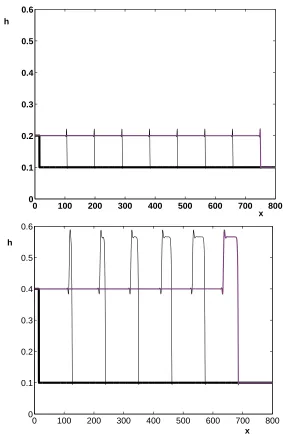
Figure 2.3: Two views of the Behringer thin film experiment viewed from above. The inclination angles of the substrate are 85 degrees (left) and 20 degrees (right) from horizontal. Note the fingering appears only in the left photograph and the broadened capillary ridge appears only on the right.[69]
wave moving at one uniform speed with a uniform profile, they observed a widening
capillary ridge, indicating that within the capillary ridge the downstream fluid was
moving faster than the upstream fluid. This could not be explained by the theory of
classical waves developed by Lax and Ole˘inik in the 1950’s [43, 54, 55].
In addition to the widening capillary ridge, Cazabat observed a second unexpected
phenomenon. Gravity-driven films exhibit a fingering instability at the leading edge,
much like paint drips down a wall. For large inclination angles (more vertical),
Caz-abat observed the expected fingering instability. However, for smaller inclination
angles, the fingers were no longer present and the film advanced with a straight and
stable leading edge. The suppression of the fingering instability occurs because of the
opposing forces in the experiment, This phenomenon is described in more detail in
Figure 2.3 provides two views of the experiment from above. The reservoir is at
the bottom and the leading edge of the film is near the top. The black areas of the
pictures are interference fringes that are very close, which indicate steep gradients.
The figure on the left is a photograph taken when the substrate has a steep inclination
angle. Note the fingering at the leading edge of the film. The figure on the right is
a photograph taken when the substrate has a shallow inclination angle. Note the
lack of fingering at the leading edge of the film and the broadening capillary ridge.
For industrial applications in which predictable and even coatings of a surface are
required, such a lack of fingering is highly desirable. Consequently, an understanding
of why the fingers disappeared and under what circumstances they could be eliminated
was of both theoretical and practical interest.
Cazabat communicated the strange results to Andrea Bertozzi at Duke University,
who had previously published results with M.P. Brenner on linear stability and
tran-sient growth in thin films [6]. Bertozzi formed a collaboration with Andreas M¨unch
visiting Duke from Technische Universit¨at M¨unchen in Germany and my advisor,
Michael Shearer, from North Carolina State University to explain the two
phenom-ena. They proved the existence in the film of both classical and non-classical waves, which Shearer understood from other contexts. [64, 29].
Experiments in thin films have been continued in both Physics and Engineering
departments at a number of universities. In addition to the laboratories of Cazabat
Technology and Schatz at the Georgia Institute of Technology continue to provide new
information about thin liquid films. The mathematical study of thin liquid films also
remains a subject of intensive research. Recent findings appear in the proceedings
of a conference at the Banff International Research Station in 2003 [8] as well as
the proceedings of the American Physical Society Division of Fluid Dynamics annual
meeting, 2004 [20].
The successful international collaboration between Cazabat’s group in Europe and
Bertozzi’s group in the United States brought physicists and mathematicians together
to explain the mysterious experimental results and paved the way to a deeper
under-standing of the role of waves in thin liquid films. The work in this thesis continues
the exploration of thin liquid films: contact line issues, kinetics and nucleation, wave
structures and discontinuous solutions, localized forcing and the effect of surfactant
2.2
Derivation of the Scalar Thin Film Equation
This section contains a derivation of the equations that describe the thin film flow in
the Marangoni and gravity-driven experiment. It begins with a non-dimensionalization
of the Navier-Stokes equations, employs the lubrication approximation and
incorpo-rates a depth averaged velocity for the speed of the film. Appropriate boundary
conditions lead to a scalar PDE, the thin film equation.
2.2.1
Velocity of the Flow and Gravity
In the most general sense, the velocity vector for the flow~u depends on three spatial
directions and time: ~u= (u(x, y, z, t), v(x, y, z, t), w(x, y, z, t)). We assume our flow is
uniform in the transverse (y) direction. Note that this would not be true for fingering,
but this thesis does not address the topic. Therefore the components of the flow are:
u=u(x, z, t), v = 0, w=w(x, z, t). (2.1)
We split gravity into two components, one tangent to the substrate, gtan, and one
perpendicular to the substrate,gperp. The inclination angle of the substrate, measured
from horizontal, is denoted by α. Therefore the two components of gravity are gtan=
a
a a a b
b b
g_tan
g_perp
g
Figure 2.4: Diagram of the inclined substrate explaining decomposition of gravity
g into tangential component gtan and normal component gperp, where a = α is the
inclination of the solid substrate and b is the complement of a.
2.2.2
Navier-Stokes Equations
Since we have assumed there is no velocity in they-direction,v = 0, we have only two
of the usual three Navier-Stokes equations, plus the continuity equation that states
the flow is incompressible. We begin with the assumption that the density ρand the
viscosity µare constant. Experimental results of Sur (see Figure 2.1) indicate only a
slight variation of temperature from the modeling assumption of linear and constant
temperature regimes. Thus the Navier-Stokes equations are
ρ(ut+uux+wuz) = −Px+µ(uxx+uzz)−ρgsinα (2.2)
ρ(wt+uwx+wwz) = −Pz +µ(wxx+wzz)−ρgcosα (2.3)
ux+wz = 0 (2.4)
where subscripts denote partial derivatives.
define characteristic variables:
L = characteristic length (x-direction) (2.5)
H = characteristic height (z-direction) (2.6)
U = characteristic velocity in the x-direction (2.7)
W = characteristic velocity in the z-direction (2.8)
T = characteristic time (2.9)
which will be used for dimensional analysis and later non-dimensionalization.
2.2.3
The Lubrication Approximation
The lubrication approximation takes advantage of the thinness of the film by
employ-ing a small parameter:
H
L =.
In the thin film experiments of Cazabat and Sur, epsilon is on the order of 10−6meters
(a micrometer).
reduce to the Stokes equations:
0 = −Px+µ(uxx+uzz)−ρgsinα (2.10)
0 = −Pz +µ(wxx+wzz)−ρgcosα (2.11)
ux+wz = 0 (2.12)
Before applying boundary conditions, we drop the terms containing uxx,wxx and
wzz by comparing their size (in terms of powers of ) to other terms in the Stokes
Equations. In particular, if
x=Lx,ˆ z =Hz,ˆ u=Uu,ˆ and t =Tˆt, (2.13)
the incompressibility condition, ux+wz = 0, gives us the following scaling for w:
w= HU
L wˆ =Uwˆ (2.14)
and we see that
wxx =
U
L2wˆxx <<
U
H2wˆzz <<
U
H2uˆzz =uzz. (2.15) and
uxx=
U
L2uˆxx <<
U
dimensional equations
Px = µuzz−ρgsinα (2.17)
Pz = −ρgcosα (2.18)
ux+wz = 0 (2.19)
2.2.4
Boundary Conditions
Normal stress boundary condition
The normal stress (pressure) boundary condition equates the force exerted by the
membrane at the liquid-air interface z =h(x, t) on the fluid below with the effect of
surface tension, through the curvature of the free surface:
P −Patm =−γκ.
Here, the curvature is κ = hxx
(1+(hx)2)32 and surface tension is denoted by γ. The
expression for curvature simplifies in the lubrication approximation since
hx ≈
H
As we linearize the expression for curvature, we keep the smallhx, but drop the term
h2
x <<1. In dimensional form the curvature is
κ= hxx
1 + (hx)2
32 ≈
hxx.
Thus our normal stress boundary condition is
P −Patm =−γhxx atz =h(x, t). (2.20)
Tangential stress boundary condition
We choose the following linear equation of state to relate the surface tension gradient
to the temperature gradient:
Γ(Ts) =γ0 −τ(Ts =T∞), (2.21) in which Ts is the temperature at the surface, T∞ is the ambient temperature, τ is the surface tension gradient and γ0 is a base value of surface tension. The surface
tension gradientτ is taken to be a constant, a reasonable approximation over a small
range of Ts about T∞. Note that τ is constant. In the experiments of Cazabat and Sur, an approximately constant surface tension gradient is achieved by taking data
in a region of the substrate where the temperature gradient is linear.
assumption that we drive the film with a constant surface stress, which couples the
gradient in surface tension τ to the shear component of stress Tzx in the flow.
τ =Tzx= 2µDzx (2.22)
The velocity gradient tensor, D, also known as the strain rate tensor, is the time
derivative of the deformation gradient. The tensor describes how the fluid moves
with respect to itself, and relates stress to strain in the law given above. The strain
rate tensor has the form
D = 1
2(∇u+∇u
T)
= 1 2
ux 0 uz+wx
0 0 0
uz+wx 0 wz
therefore Dzx= 12uz+O() and our tangential stress condition takes the form
No slip boundary condition
The no slip boundary condition assumes that the liquid at the liquid-solid interface
is not moving. This is expressed in the boundary condition:
u= 0 at z = 0. (2.24)
Note that this will be generalized in the Navier slip model.
2.2.5
Integrating the PDEs
To derive the final dimensional form of the thin film equation, we will integrate three
times and employ the boundary conditions to determine constants of integration.
We begin by integrating the second equation for pressure from (2.18) with respect
toz:
P(x, t) = Z z
0
Pzdz˜=−
Z h
z −
ρgcosαdz˜=ρgcosα(h−z) +C1 (2.25) We determine C1 using the normal stress boundary condition (2.20) which yields
P(x, t) = ρgcosα(h−z) +Patm−γhxx (2.26)
into the first pressure equation (2.19).
µuzz =ρgcosαhx−γhxxx+ρgsinα (2.27)
We integrate twice with respect to z to derive an expression for the velocity u. After
the first integration we have the following equation:
µuz = (ρghxcosα−γhxxx+ρgsinα)z+C2. (2.28) We solve for C2 using the tangential stress boundary condition (2.23) which yields
C2 =τ −(ρghxcosα−γhxxx+ρgsinα)h. (2.29)
The second integration with respect to z yields
µu= (ρghxcosα−γhxxx+ρgsinα)
z2
2 +C2z+C3. (2.30)
where C3 = 0 due to the no slip boundary condition (2.24. This provides our final
equation for the velocity u(x, z, t):
u= 1
µ
(ρghxcosα−γhxxx+ρgsinα)
z2 2 −hz
+τ z
2.2.6
Depth-Averaged Velocity and Flux
Q
We average the velocity u over the thickness of the film, h. The velocity profile is
parabolic, but the film is thin, so we can average it. Note that this means that the
tangential gravity term containsh3, since we integrateh2 once. We regard the flux as
the width times the depth-averaged velocity in which the first term is due to surface
tension, the second term is due to curvature, the third term is due to the normal
component of gravity and the fourth term is due to the tangential component of
gravity:
Q= 1
h
Z h 0
udzˆ= 1
hµ
τ h2 2 +
γh3h
xxx
3 −
ρgh3h
xcosα
3 −
ρgh3sinα 3
(2.32)
If we assume that τ > 0, then the fluid is pulled up the plate by surface tension and
down the plate by the tangential component of gravity.
2.2.7
Conservation of Mass
Conservation of mass dictates that the change in the height of the fluid, ∂h
∂t is balanced
by the change in the amount of fluid at the boundary. We consider a slice of the fluid
with fluid flowing in at x to fluid flowing out at x+ ∆x.
(∆xh)t =
Z h 0
u(z, x)dz−
Z h(x+∆x) 0
Dividing by ∆x, we obtain the desired conservation law in the limit ∆x→0:
ht + (hQ)x = 0 (2.34)
Substituting the expression for the flux (2.32) leads to the dimensional form of the
thin film equation:
ht+
τ h2 2µ −
h3ρgsinα 3µ
x
= −H
4h3(γh
xx)x
3Lµ +
ˆ
h3ρgcosαhˆ ˆ x 3µ ! ˆ x (2.35)
2.2.8
Non-dimensionalization
To non-dimensionalize equation (2.35), we employ the non-dimensional variables
(de-noted by hats) defined in equations (2.9) and (2.13) to obtain
H T hˆˆt+
1
L
H2τhˆ2 2µ −
H3ˆh3ρgsinα 3µ ! ˆ x = 1 L −
H4γhˆ3ˆh ˆ
xxˆxˆ 3L3µ +
h3ρgcosαh ˆ x 3µ ! ˆ x (2.36)
Now we define the characteristic variables by balancing terms. First we balance the
tangential gravity and Marangoni terms to defineH. Note that the independent and
dependent variables are all order 1. We obtain the following equation for H
τ H2 2µ =
H3ρgsinα
3µ , thus H =
3τ
Next we defineLas the capillary length such that the Marangoni and surface tension
effects balance:
τ H2 2µ =
γH4
3µL3 thus L=
3γτ
2ρ2g2sin2α 13
(2.38)
Now choose the time scale T so that gravity, Marangoni and surface tension forces
balance:
H
T =
τ H2
2Lµ thus T =
2µ τ2
4γτ ρgsinα
9
13
(2.39)
We substitute the expressions for H,LandT into (2.36) and drop the hats to obtain
the dimensionless equation thin film equation (with no slip at the substrate):
ht+ h2−h3
x =D h
3h
x
x− h
3h
xxx
x
in which D = ρgT H3µL3cos2 α is typically small since the effects of the normal component
of gravity for a thin film are negligible. Henceforth we take D = 0. Thus we have
derived the scalar dimensionless thin film equation
Comparison of Contact Line
Models
3.1
Introduction
In attempting to resolve the well-known stress singularity [21] at a moving contact
line, the leading edge of a liquid spreading over a dry solid surface, two strategies
are often proposed. One strategy is to introduce a very thin precursor layer of fluid,
which is assumed to move hydrodynamically with the bulk fluid behind the contact
line. In such aprecursor model, the contact slope can be associated with the steepest part of the free boundary, i.e., the liquid-air interface, which of course does not come
into contact with the solid surface. In the second type of model, the free surface is
assumed to achieve contact with the solid surface, but a boundary condition between
the fluid and the solid surface permits a small amount of slip of the fluid on the solid,
in contrast with the usual no-slip boundary condition. Such a boundary condition
was introduced by Navier [52] at the start of a debate concerning suitable
liquid-solid boundary conditions [25], leading eventually to the conclusion that the no-slip
boundary condition is realistic for a viscous fluid. The so-calledNavier slip condition was taken up much later in the context of contact lines [34]; we use the so-called
singular slip of Greenspan [25] to formulate the Navier slip model.
In this chapter, we explore the connections between these two models by doing
numerical experiments. Specifically, we simulate traveling wave solutions of equations
obtained from the lubrication approximation to the Navier-Stokes equations. We
compare contact slopes for the two models, and their dependence upon parameters
such as the upstream film height and the precursor height. We restrict attention to
a thin film being driven up a solid flat surface by a gradient in surface tension. The
surface tension gradient is induced in experiments by a temperature gradient [12],
[69], thereby creating a Marangoni surface stress that provides the driving force. In
the absence of Marangoni force, a similar study was undertaken by Tuck and Schwartz
[70]. In our case, with Marangoni force, we find different behavior, some of which was
observed in [10]. Preliminary results in [10] indicated a bounded interval of contact
slopes for specific choices of parameters. In this chapter, we explore systematically
As derived in the previous chapter, the thin film PDE is of the form (cf. [7]):
ht+f(h)x =−(C(h)hxxx)x, (3.1)
in which f and C are smooth functions that are positive for h >0; they incorporate
effects of gravity, surface tension and the Marangoni force. (We have also dropped
second order diffusive terms from (3.1) as they are small [51].)
We seek traveling wave solutions, h(x, t) = ˜h(x−st) of (3.1), in which s is the speed of the traveling wave. By substitution into the PDE (3.1) and one integration,
we arrive at a third order ODE for h(ξ) (dropping the tilde), where ξ =x−st:
h000 = sh−f(h)−shm+f(hm)
C(h) , (3.2)
in which 0 = d
dξ, hm>0 is the upstream height, and s is the wave speed.
The computer program we use to understand the structure of solutions of equation
(3.2) is modeled on that employed by Buckingham in [10]. The new code enables us
to explore stable and unstable manifolds of the vector field associated with (3.2) with
much greater efficiency than earlier procedures, simply by automating much of the
selection of parameters. We use the program not only to compare the two models,
and nucleation condition postulated in [45] for the underlying scalar conservation law
ht+f(h)x = 0. (3.3)
3.2
The ODE Models
3.2.1
The Navier Slip Model
For the Navier slip model, we adopt the singular slip form of Greenspan [25], which
states that at the fluid-solid interface, the fluid velocity u parallel to the interface
should be proportional to the strain rate in the fluid, with a coefficient that depends
on the height of the film but which blows up at the contact line. Specifically,
u=ηhn−2∂u
∂z on z = 0.
Note that this is different from (2.24), the no-slip boundary condition.
Here, 0 < n ≤ 2 is an empirical parameter; we take n = 1, as suggested in [25]; The value n = 2 is considered by Hocking and others [32]. The parameter η > 0 is
generally taken to be very small; ηhn−2 has the dimension of length; consequently, for n = 1, η has the dimension of (length)2; the length scale for the slip is taken to
be at least an order of magnitude smaller than the maximum thickness of the film.
as in [7]):
C(h) =h3+βh, f(h) = h2−h3+2
3β−βh, (3.1) where β >0 is a small parameter related to η. Since the fluid surface makes contact
with the solid surface, the height becomes zero at some point, which we can take to
be the origin. Correspondingly, we impose the boundary conditions
h(−∞) = lim
ξ→−∞=hm, h(0) = 0
on traveling waves. Conservation of mass relates the wave speed s to the upstream
height alone, since this speed is also the speed of the contact line, and hence is the
(depth averaged) velocity of the fluid parallel to the solid surface:
s= f(hm)
hm
. (3.2)
Consequently, the terms−shm+f(hm) in (3.2) are zero for the Navier slip model.
3.2.2
The Precursor Model
In the precursor model, we impose the no-slip boundary condition (2.24) between the
fluid and solid surface, corresponding to β = 0 in (3.2). Thus, the functions in (3.1)
simplify to
Moreover, the fluid surface does not make contact with the solid surface, so the height
remains positive. Correspondingly, we impose boundary conditions
h(−∞) = lim
ξ→−∞=hm, h(∞) = limξ→∞=hb,
where hb < hm is the precursor height. Conservation of mass relates the wave speed
s to both the upstream and downstream heights:
s = f(hm)−f(hb)
hm−hb
. (3.4)
3.2.3
Comparison
The two models differ in their significant parameters (see Table 3.1). In the Navier
slip model, the parameters are hm and β (the slip parameter), whereas in the
pre-cursor model, there are also two parameters, hm and hb. However, the boundary
condition h(0) = 0 from the Navier slip model is at a singular point for the ODE;
correspondingly, there is an additional degree of freedom in the ODE solutions for
the Navier slip model compared with the precursor model. To compare film profiles
for the two models, we use the technique proposed by Tuck and Schwartz [70], in
which a profile with Navier slip corresponds to one with a given precursor height if
Table 3.1: Model Specifications
Navier Slip Precursor
slip parameter β >0 β = 0
boundary conditions h(−∞) =hm,h(0) = 0 h(−∞) = hm, h(∞) =hb
wave speed s = f(hhm)
m s=
f(hm)−f(hb)
hm−hb flux function f(h) =h2−h3+ 2
3β−βh f(h) =h 2−h3
3.2.4
Equilibria
In this section, we consider equation (3.2) as a first order system. Equation (3.2) is
h000 =g(h), where g(h) = sh−f(h)−shm+f(hm)
h3+βh , (3.5)
which is equivalent to the first order system
h0 = u (3.6)
u0 = v
v0 = g(h).
Equilibria of the system are of the form (h, u, v) = (¯h,0,0) with g(¯h) = 0, i.e.,
s(¯h−hm) = f(¯h)−f(hm). (3.7)
For fixed hm and s, this equation is represented graphically in Figure 3.1 as the
For the Navier slip model, the flux function f(h) =h2−h3+2
3β−βh intersects the y-axis at 23β, and the h axis at h= 1− 13β+O(β2). Equation (3.2) implies the line with slope s passes through the origin. In the precursor model, the graph of the flux
function intersects the origin and the line with slope s does not, due to (3.4). The
line can intersect the flux function as many as three times leading to three equilibria
we label from the left B (bottom), M (middle) and T (top).
Figure 3.1: Flux functions, line with slope s and equilibria. Navier slip (β = 0.01 shown); Precursor model (β = 0).
Let ¯h satisfy (3.7). Linearizing (3.5) abouth= ¯h, we obtain
w000 = d(¯h)w, d(¯h) = dg
dh(¯h) .
The characteristic equation λ3 =d(¯h) has three solutions, a complex conjugate pair
λ± =α±iγ and a real solutionλR= (d(¯h))
1
3.The three eigenvalues are spread evenly
around the circle with radius |λR| in the complex plane. Since
g0(¯h) = s−f0(¯h) ¯
at an equilibrium, we read off from Figure 3.1 thatg0(¯h)>0 at B and T, whileg0(¯h)<
0 at M. Consequently, B and T have one-dimensional unstable manifolds WU(B),
WU(T) and two-dimensional stable manifolds WS(B), WS(T). Similarly, M has
a two-dimensional unstable manifold WU(M) and one-dimensional stable manifold
WS(M).
Remark: In the Navier slip model, we consider trajectories that connect to h = 0.
These are trajectories originating at the middle equilibrium M rather than at B or T;
while there may be trajectories from these other equilibria, they are less significant for
our purpose, as there are fewer such trajectories: the unstable manifolds from B and
T are one dimensional, whereas the unstable manifold from M is two-dimensional. A
consequence is that even for the Navier slip model we consider parameter values for
which there are three equilibria.
To capture the two-dimensional invariant manifold of an equilibrium (¯h,0,0), we
set initial conditions on the tangent plane at (¯h,0,0). The tangent plane is generated
by solutions of the linear system
ˆ
h0 = ˆu
ˆ
u0 = ˆv
ˆ
corresponding to the complex conjugate eigenvalues λ±=α±iγ. Thus, ˆ h ˆ u ˆ v
(ξ) = aeαξ(cosγξv1−sinγξv2) (3.8)
where v1 = 1 α
α2−γ2
and v2 = 0 α 2αγ
generate the tangent plane.
Consider the unstable case, in which α >0. In choosing initial data for the ODE
simulation, we take a radial line in the tangent plane, i.e., a straight line emanating
from the equilibrium, and limit initial points to points on the line between successive
crossings of a single trajectory spiraling out from or into the equilibrium. From (3.8),
successive crossings occur at times differing by 2γπ; correspondingly
(ˆh,u,ˆ ˆv)(ξ+ 2π/γ) =e2παγ (ˆh,u,ˆ vˆ)(ξ).
Thus, if we select one pointP0 in the tangent plane, we capture all trajectories in the
two-dimensional manifold by selecting initial data on the line between (¯h,0,0) +P0
and (¯h,0,0) +e2παγ P0. (See Figure 3.2, in which the equilibrium is labeled ¯h, and the
two points are labeled ¯h+P0,¯h+P1.) Note thatγ/α= tanπ3,so thate
2πα
ξ = 0. However, for accuracy, we need to choose P0 close to the origin, so a =a0 is
chosen to be small.
To summarize, we initiate ODE simulations at ξ= 0, with
h u v (0) = ¯ h 0 0 +a 1 α
α2 −γ2 (3.9)
Here, the parameter a is chosen in an interval [a0, a0e
2πα
γ ), in order to capture all
trajectories in the two-dimensional invariant manifold. In practice, the choice of a
is crucial, and for greater resolution, or to focus on one part of the solution set, we
often take only a small subinterval of values of a. This adjusting of a is particularly
needed in computing the stable manifold of B when hb is very small, since then the
system is very sensitive to changes in h.
3.2.5
Parameter Ranges for Equilibria
For both the precursor and Navier slip models, we consider parameter values for
which there are three equilibria. This places restrictions on the parameters, which we
describe in two lemmas.
In the Navier Slip model, there is a limited range of β for which there are three equilibria. Recall that equilibria (¯h,0,0) occur at intersections between the flux
function, f(h) and the line with slope s=f(hm)/hm through the origin. The limits
of the parameters will occur when the chord is tangent to the flux function, i.e.,
f(h) = f0(h)h.
From f(h) =h2−h3+ 2
3β−βh, this equation becomes
h3− 1
2h 2+ 1
3β = 0. (3.10)
The three roots have product −3β <0, so that when they are all real, two are positive and one is negative. The two positive roots coalesce when the minimum of the cubic
(at h= 1
3) is a root; this occurs precisely when β = 1
18 (from setting h= 1
3 in (3.10)). There is also a maximum at h = 0, at which the negative root coincides with a
positive root, for β = 0. Thus, the range for β is
0< β < 1
Now let hmin(β) < hmax(β) be positive roots of equation (3.10). Then hm is
con-strained by
hmin(β)< hm < hmax(β). (3.11)
We summarize the result as a lemma:
Lemma 3.2.1. Let hmin(β) < hmax(β) be positive roots of equation (3.10). Then
there are three equilibria 0< hb < hm < ht for the Navier slip model (3.4) if and only
if 0< β < 181 ; consequently, hmin(β)< hm < hmax(β).
Finally, note that for the Navier slip model, the wave speed s depends only on
hm: s= f(hhmm).
For the precursor model (β = 0), the precursor height hb is constrained by
0< hb < 13. Here, we want three roots of the equation
f(h)−f(hb) = s(h−hb), (3.12)
but we also want hb to be the smallest root. Limits on s occur whens is the slope of
the tangent to the graph of s at an equilibrium, either at hb (for the minimum value
of s) or at a larger equilibrium. Thus smin = f0(hb) = 2hb −3h2b, and s = smax is
given by equation (3.12), together with
Equation (3.12) becomes, after dividing by h−hb 6= 0,
s=−(h2+hhb+h2b) +h+hb. (3.14)
Solving (3.13), (3.14), we find s = smin and h = hb, or s = smax = 14 + 12hb − 34h2b
and h= 1/2(1−hb). Thus the constraints on s and hm are specified in the following
lemma:
Lemma 3.2.2. For the precursor model (3.5 with β = 0), there are three equilibria 0< hb < hm < ht if and only if2hb−3h2b < s < 14+
1 2hb−
3 4h
2
b,hb < hm <1/2(1−hb),
and 0< hb < 13.
Remark: For the Navier slip model, we trace trajectories in WU(M), and
measure the most negative slope of those that go to h = 0 at a finite value of
ξ. As we will see in the following section, these trajectories require that WU(M)
and WS(B) intersect. As h
m is increased, these manifolds eventually separate at
hm = h∗(β) < hmax(β).1 Thus, we find trajectories for hm in a range even more
restricted than calculated in (3.11):
hmin(β)< hm < h∗(β). (3.15)
In the precursor model, we want trajectories that lie in bothWU(M) andWS(B), i.e.,
trajectories (in WU(M)∩WS(B)) that are heteroclinic orbits from M to B. Again,
separation of WU(M) and WS(B).
3.3
Numerical Experiments
The overall goal of the numerical experiments is to determine the effective contact
slope for each of the two models, and to determine the effect of varying parameters
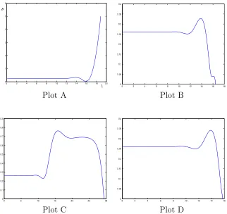
such as hb, hm and β. The effective contact slope is measured as the most negative
value ofh0 for a single trajectory.
To compute trajectories, we used the implicit Adams method in LSODE, the
Livermore Stiff ODE solver [58]. This solver is implemented with variable step size
and variable order (first to twelfth).
Initial conditions (3.9) are numbered by an index j: a = j ∗δ and jstart ≤
j ≤ jstarte
2πα
γ , in which δ is the spacing between initial points, numbered by j. The
two parameters δ and jstart are used to refine calculations where needed. The
two-dimensional manifolds WU(M), WS(B) are visualized by computing their
intersec-tions with a Poincar´e section, h = (2hm+hb)/3 (as in [7]), so that each manifold is
represented by a curve. To calculate Poincar´e sections, we use 1000 ≤ j ≤ 37623, and δ = 10−10. When refinement is needed in this process we take δ = 10−11. Note
that to calculate WS(B) we integrate backwards in ξ..
Parameter choices for for comparison of the two models, extending the range in
[10], are shown in Table 3.1. The remaining parameters in the model,hb andsfor the
Table 3.1: Parameter Specifications
hm 0.26, 0.28, 0.30, 0.32
Navier slip model: β 0.007, 0.01, 0.013
Precursor model (β = 0): hb 0.03,0.033,0.035,0.04,0.045,0.05,0.055,0.06
in Table 3.1. The values of hb in the precursor model are chosen to be small enough
to be in a realistic range; although smaller values would be desirable, simulations
become unreliable at very small values of h.
3.3.1
Phase Portraits and the Poincar´
e Section
Since the ODEs for the two models have a similar structure, it is not surprising that
their phase portraits are qualitatively similar. In Figure 3.1, we show a Poincar´e
section for the Navier slip model on a scale that illustrates the general structure of
the manifoldsWU(M), WS(B).(The gaps aroundh0 = 0 correspond to the manifolds becoming tangent to the planeh=constant; they can be made smaller by refining the
initial data.) In Figure 3.3.1, we show intersections in the Poincar´e section between
WU(M) and WS(B) on a larger scale, ash
b varies from 0.01 to 0.033 in the precursor
model. Ashb increases, we observe the line of dots representing trajectories inWS(B)
pull through the spiral ofWU(M), with varying numbers of intersections. Note that
the smaller values ofhb fall outside the range for comparison of the two models given
in Table 3.1. Specifically, for hb = 0.01, there are no trajectories from M to B so
we cannot calculate contact slopes for comparison with the Navier slip model. The