Obstacle avoidance of mobile robots using modified artificial potential field algorithm

(1)

R E S E A R C H

Open Access

Obstacle avoidance of mobile robots using

modified artificial potential field algorithm

Seyyed Mohammad Hosseini Rostami

1

, Arun Kumar Sangaiah

2

, Jin Wang

3*

and Xiaozhu Liu

4

Abstract

In recent years, topics related to robotics have become one of the researching fields. In the meantime, intelligent mobile robots have great acceptance, but the control and navigation of these devices are very difficult, and the lack of dealing with fixed obstacles and avoiding them, due to safe and secure routing, is the basic requirement of these systems. In this paper, the modified artificial potential field (APF) method is proposed for that robot avoids collision with fixed obstacles and reaches the target in an optimal path; using this algorithm, the robot can run to the target in optimal environments without any problems by avoiding obstacles, and also using this algorithm, unlike the APF algorithm, the robot does not get stuck in the local minimum. We are looking for an appropriate cost function, with restrictions that we have, and the goal is to avoid obstacles, achieve the target, and do not stop the robot in local minimum. The previous method, APF algorithm, has advantages, such as the use of a simple math model, which is easy to understand and implement. However, this algorithm has many drawbacks; the major drawback of this problem is at the local minimum and the inaccessibility of the target when the obstacles are in the vicinity of the target. Therefore, in order to obtain a better result and to improve the shortcomings of the APF algorithm, this algorithm needs to be improved. Here, the obstacle avoidance planning algorithm is proposed based on the improvement of the artificial potential field algorithm to solve this local minimum problem. In the end, simulation results are evaluated using MATLAB software. The simulation results show that the proposed method is superior to the existing solution.

Keywords:Obstacle avoidance, Navigation, Artificial potential field, Mobile robot

1 Introduction

An intelligent mobile robot must reach the designated targets at a specified time. The robot must determine its location relative to its objectives at each step and issue a suitable strategy to achieve its target. Informa-tion about the environment is also needed to avoid obstacles and design optimal routes. In general, the objectives of this study are (1) improving the APF algorithm in order to trace the path and avoid obsta-cles by a mobile robot and (2) comparing the per-formance and efficiency of the proposed algorithm with the previous method, APF algorithm. In the real world, it gets a lot of use. For example, we have an automatic ship that we want to avoid collision with obstacles and to take the best possible route for a

low cost. It is possible to detect the distance between the robot with the target and obstacles with the help of the sensor. However, the sensor discussion is sep-arate from this article.

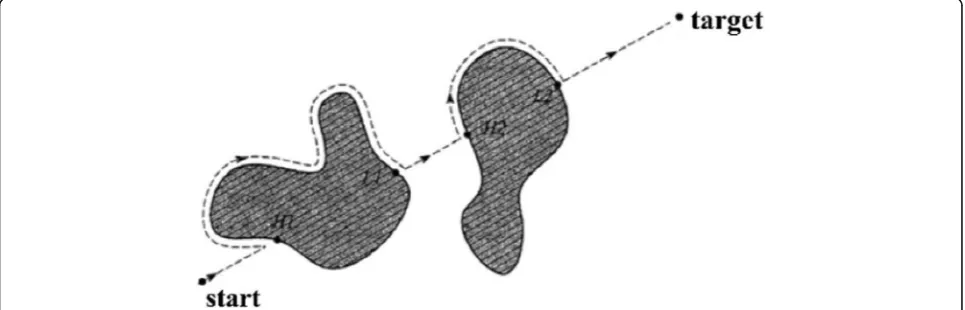
Mobile intelligent robot is a useful tool which can lead to the target and at the same time avoid obsta-cles facing it [1]. There are conventional methods of obstacle avoidance such as the path planning method [2], the navigation function method [3], and the opti-mal regulator [4]. The first algorithm that was pro-posed for the discussion of obstacle avoidance is the Bug1 algorithm. This algorithm is perhaps the sim-plest obstacle avoidance algorithm. In the first algo-rithm, Bug1, as shown in Fig. 1, the robot completely bypassed the first object, and then, it leaves the first object and performs at the shortest distance from the target. Of course, this approach is very inefficient, but it ensures that the robot is reachable for any purpose. In this algorithm, the current sensor readings play a

© The Author(s). 2019Open AccessThis article is distributed under the terms of the Creative Commons Attribution 4.0 International License (http://creativecommons.org/licenses/by/4.0/), which permits unrestricted use, distribution, and reproduction in any medium, provided you give appropriate credit to the original author(s) and the source, provide a link to the Creative Commons license, and indicate if changes were made.

* Correspondence:[email protected]

3_{School of Computer & Communication Engineering, Changsha University of}

Science & Technology, Changsha, China

(2)

key role. The weakness of this algorithm is the exces-sive presence of the robot alongside the obstacle [5].

In the second algorithm, Bug2, as shown in Fig.2, the robot moves on the starting lineup to the target, and if it sees the obstacle, it will round the obstacle, and when it again reaches a point on the line between the start to the target, it leaves an obstacle. In this algorithm, the robot spends a lot of time moving along the obstacle, but this time is less than the previous algorithm [5].

In the following, Mr. Khatib introduced an algorithm called APF in 1985 [6]. This algorithm considers the robot as a point in potential fields and then combines stretching toward the target and repulsion of obstacles. The final path of the output is the intended path. This algorithm is useful given that the trajectory is obtained by quantitative calculations. The problem is that in this algorithm, the robot can be trapped in the local mini-mum of potential fields and cannot find the path; hence, in this paper, some amendments have been made to

resolve this issue, which is discussed in Section3. Subse-quently, in March 1991, Borenstein and Koren presented vector histogram field algorithm (VHF) [7]. In this algo-rithm, with the help of one of the distance sensors, a planar map of the robot environment is prepared; in the next step, this planar map is translated into a polar histogram. This histogram is shown in Fig.3, where the

x-axis represents the angles around the obstacle and the y-axis represents the probability of an obstacle at the desired viewing angles. In this polar map, the peaks represent bulky objects and valleys represent low-volume objects; valleys below the threshold are suitable valleys for moving the robot; finally, the suit-able valley which has a smaller distance to the target is selected from the valleys, and the position of this valley determines the angles of motion and speed of the robot [7].

Improvements on VFH led to the introduction of VFH‐ and VFH+ [8]. The next algorithm is the sensor

Fig. 1Bug1 algorithm with two points H1 and H2 as collision points. L1 and L2 are selected as the exit point

(3)

fusion in certainty grids for mobile robots which is one of the well-known, powerful, and efficient algorithms for using a multi-sensor combination to identify the envir-onment and determine the direction of movement. In this algorithm, the robot’s motion space is decomposed into non-overlapping cells and is provided with a graph-ical motion environment, and then based on the algo-rithms for searching the graph, the path of the movement is determined [9]. In the following, the Fol-low the Gap method (2012) was proposed [10]; in this algorithm, the robot calculates its distance with each obstacle. The robot can know the distance between ob-stacles by knowing its distance with each obstacle. The robot then detects the greatest distance between obsta-cles and calculates the center angles of the empty space. After the central angular momentum, the robot calcu-lates the empty space, combines it with the target angle, and shows the ending angle. Obviously, in this combin-ation, it is done on a weight basis, so that the obstacles that are closer to the robot are weighing more because their avoidance is a priority for the robot. Figure4shows how this method works.

Fuzzy logic and neuro-fuzzy networks can also be used to avoid obstacles. In this regard, fuzzy logic can be helpful in solving the problems caused by the ocean flow in the underlying surfaces [11]. It should be noted that the algorithms discussed in the research background for avoiding an obstacle are different from each other, and each algorithm has proposed a separate and new method for avoiding obstacles. So far, novel methods to avoid obstacles in addition to the mentioned methods are also presented [12–16]. In the following section, we first in-vestigate the artificial potential field algorithm and then modify this algorithm in Section 3. In [17], the state-dependent Riccati equation (SDRE) algorithm is studied on the motion design of cable-suspended robots with uncertainties and moving obstacles. A method for controlling the tracing of a robot has been developed by the SDRE. In [18], the fuzzy logic method is used to

predict the movement of obstacles and accelerate the linear velocity of the robot. In this paper, the movement trend of the obstacle in approaching the robot is divided away from the robot and translated by the robot. With respect to the three trends, the robot can increase the velocity, decrease the velocity to pass by the obstacle, or stop to wait for the obstacle to pass. Some simulation re-sults show that the proposed method can help the robot avoid an obstacle without changing the initial path. In [19], we have a four-dimensional unmanned aerial vehi-cle’s platform equipped with a miniature computer equipped with a set of small sensors for this work. The platform is capable of accurately estimating the precision mode, tracking the speed of the user, and providing un-interrupted navigation. The robot estimates its linear velocity by filtering a Kalman filter from the indirect and optical flow with the corresponding distance measure-ments. In [20], a new method for defining the path in the presence of obstacles is proposed, which describes the curve as a two-level intersection. The planner, based on the definition of the path along with the cascaded control architecture, uses a non-linear control technique for both control loops (position and attitude) to create a framework for manipulating multivariate behavior. The method has been shown to be able to create a safe path based on perceived obstacles in real time and avoiding collisions. Li et al.[21] refer to the tracking control of Euler-Lagrange system problems with external impedi-ments in an environment containing obstacles. Accord-ing to a new slidAccord-ing discovery, a new trackAccord-ing controller is proposed to determine the tracing, convergent errors reach zero as infinite time. In addition, based on the non-destructive sliding terminal, a simultaneous control algorithm with time constraints has also been developed to ensure that tracking errors are approaching a re-stricted area close to the source at a given time. By introducing multi-purpose collision avoidance functions, both controllers can ensure that the obstacle is avoided. In [22], the mobile sensor deployment (MSD) problem

(4)

had been studied in mobile sensor networks (MSNs), aiming at deploying mobile sensors to provide target coverage and network connectivity with requirements of moving sensors. This problem is divided into two sub-problems, the Target COVerage (TCOV) problem and Network CONnectivity (NCON) problem. For the TCOV problem, it is proved that it is NP-hard. For a special case of TCOV, an extended Hungarian method is provided to achieve an optimal solution; for general cases, two heuristic algorithms are proposed based on the clique partition and Voronoi diagram, respectively. For the NCON problem, at first, an edge constrained Steiner tree algorithm is proposed to find the destina-tions of mobile sensors, and then, we used extended Hungarian to dispatch rest sensors to connect the net-work. Theoretical analysis and simulation results have shown that compared to extended Hungarian algorithm and basic algorithm, the solutions based on TV-Greedy have low complexity and are very close to the optimum. In [23], a novel approach is presented to obtain the opti-mal performance bounds for a multi-hop multi-rate wireless data network. First, the optimal relay place-ments are determined for a target terminal located at a distance D away from the access point. Second, for a general analytical PHY layer throughput model, the maximum achievable MAC throughput is determined as

a function of the number of relays for a target located at distanceD.

In all the research mentioned above, the local mini-mum problem has not been solved, and we designed the modified APF method to solve this problem. In this paper, in the second part, firstly, the previous method of APF algorithm is presented. Then, in Section3, the APF method is modified to remedy the defects of this method.

2 Problem statement and formulation 2.1 Methods

The artificial potential field model suggested by Khatib [6] is a typical field model (Fig.5). In the artificial poten-tial field model,T represents the target for the robot to generate attraction and O represents the obstacles that produce repulsion for the robot.

In a planar space, the problem of avoiding the collision of a robot with an obstacle O is shown in Fig. 5. If XD

indicates the target position, the control of the robot with respect to the obstacle Ocan be done in the artifi-cial potential as follows:

UALLð Þ ¼X UAð Þ þX URð ÞX ð1Þ

where UA,UR, andUALLrespectively represent attraction

(5)

potential energy, repulsive potential energy, and artificial potential field. Then its gradient function can be written as follows:

FALL¼ FAþFR ð2Þ

FA¼−grad½UAð ÞX ð3Þ

FR¼−grad½URð ÞX ð4Þ

where FA is the attraction generated by the robot to

reach the target position of XD and FR represents the

force created byUR(X), which is caused by the repulsion of the obstacle. FA is proportional to the distance be-tween the robot and the target. Then, the attraction kS factor is also considered, and the attraction potential

UA(x) field is simply obtained as follows:

UA¼ 1 2kSRA

2 _ð₅_Þ

Additionally,UR(X) is a non-negative, non-linear func-tion that is continuous and differentiable, and its poten-tial penetration must be limited to a particular region around the obstacle without undesired turbulence forces. Therefore, the equationUrep(X) is as follows:

URð Þ ¼X 0:5Z

the target position. RA¼

ffiffiffiffiffiffiffiffiffiffiffiffiffiffiffiffiffiffiffiffiffiffiffiffiffiffiffiffiffiffiffiffiffiffiffiffiffiffiffiffiffiffi ðX−XDÞ2þ ðY−YDÞ2

q

is the shortest distance between a robot and a target in a

pla-nar space, Z is the repulsive increase factor, RR

¼ ffiffiffiffiffiffiffiffiffiffiffiffiffiffiffiffiffiffiffiffiffiffiffiffiffiffiffiffiffiffiffiffiffiffiffiffiffiffiffiffiffiffiffiffiffiffiffiðX−XOBÞ2þ ðY−YOBÞ2

q

is the shortest distance

be-tween the robot and obstacles in the planar space, and

G0 represents a safe distance from the obstacles [24]. According to the kinetic theory, the relationG0≥VMAX/

2AMAX is used, where VMAX denotes the maximum

speed of the robot and AMAX represents the maximum

speed of the acceleration (negative acceleration). So at-traction and repulsion functions are written as follows:

FA¼−∇

It is assumed that φ is the angle between theX‐axis and the line from the point of the robot to the obstacle. Then, both the repulsion components in the direction of the X‐axis and the Y‐axis can be obtained. Given θ is the angle between the X‐axis and the line from the point of the robot to the target, the attraction compo-nents in the X‐axis and the Y‐axis are considered as the following equations [24]:

FRxðX;XOBÞ ¼ FRðX;XOBÞcosφ ð9Þ

FRyðX;XOBÞ ¼ FRðX;XOBÞsinφ ð10Þ

FAxðX;XDÞ ¼FAðX;XDÞcosθ ð11Þ

FAyðX;XDÞ ¼FAðX;XDÞsinθ ð12Þ

First, the force of the repulsion and attraction in the g-axis and the v-axis are calculated, and then, f is the angle between the resulting force and the d-axis. Finally, the angle of the steering command is calcu-lated as follows:

(6)

Fx¼ FAxðX;XDÞ þ FRxðX;XOBÞ ð13Þ

The next position of the robot can be continuously calculated according to the following function until it reaches the convergence condition:

Xf ¼XþL cosδ

Yf ¼YþL sinδ

ð16Þ

whereLdenotes the step size andXfand Yfrepresented the next position of the robot. Then, if the obstacles are simple particles, the artificial potential field model is used to secure the robot to the point of the target. How-ever, there are several problems. First, the result from the sum of the two forces of attraction and repulsion in some places is zero, which results in stopping the robot moving or wandering around those points that are called local minimum. Second, when the target is surrounded by obstacles, the path cannot converge, and the robot cannot reach the target. In order to overcome these

shortcomings, Section 3 addresses the modification of

the artificial potential field algorithm.

3 Algorithm design

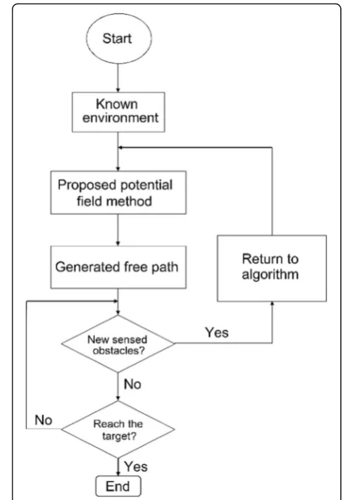
Researchers around the world have been researching about artificial potential field defects and have presented suggestions for improving this method [25–37]. Here, a regulative agent has been added to improve the artificial potential field algorithm with the target of overcoming the minimum local and inaccessible target. When the robot is close to the target, this regulative agent reduces the attraction control as a linear function, and the repul-sion decreases as a higher-order function (M≥3). A flowchart illustrating the steps of the modified APF algo-rithm is given in Fig.6.

3.1 Modified artificial potential field model

In the planar space, the modified function of the attrac-tion field funcattrac-tion is defined as follows:

UA¼ 1 2kSRA

2 _ð₁₇_Þ

The modified attraction field function is written as follows: get position.RAis the shortest distance between the robot and the target in the planar space, andRANis the regula-tive factor. The attraction function is the gradient across the attraction field, which is obtained as follows:

FA¼−∇

In the same way, the repulsive function is a negative gradient from the field of repulsion, which is obtained as follows:

(7)

FR¼ ZFR1ð Þ þX MZFR2ð ÞX RR≤G0

0 RR>G0

ð20Þ

As shown in Fig. 7, in the modified model, FR is decomposed intoFR1 and FR2, where FR1 is the compo-nent’s force in the direction of the line between the robot and the obstacle andFR2is the component’s force in the direction of the line between the robot and the target.

FR1 ¼ 1

RR− 1

G0

RAM

RA3

FR2¼ 1

RR− 1

G0

2

RAM 8

> > < > >

: ð21Þ

The two components of repulsion and attraction in the direction of the x-axis and they-axis can be obtained as follows [24]:

FRxðX;XOBÞ ¼ FRðX;XOBÞcosφ ð22Þ

FRyðX;XOBÞ ¼ FRðX;XOBÞsinφ ð23Þ Fig. 7Analysis of forces on a robot

0 1 2 3 4 5 6 7 8 9 10

X

Y

start point

target point

Simulation result of modified APF

(8)

FAxðX;XDÞ ¼FAðX;XDÞcosθ ð24Þ

FAyðX;XDÞ ¼FAðX;XDÞsinθ ð25Þ

The force of the repulsion and attraction on X‐axis and Y‐axis are calculated, and the angle δ is calculated

between the force and the X‐axis, where δis the steer-ing angle of the robot.

Fx¼ FAxðX;XDÞ þ FRxðX;XOBÞ ð26Þ

Fy¼ FAyðX;XDÞ þFRyðX;XOBÞ ð27Þ

0 500 1000

80 85 90 95 100

Number Of Steps

Ua

tt

Uattraction

0 500 1000

0 5 10 15x 10

4

Number Of Steps

U

rept

Urepulsion

0 500 1000

0 2 4 6 8 10 12x 10

4

Number Of Steps

Ua

ll

Ufinal

Fig. 9The energy amount of repulsion and attraction and their yields according to the number of steps in the artificial potential field algorithm for circular obstacles with radiusR= 0.18

(9)

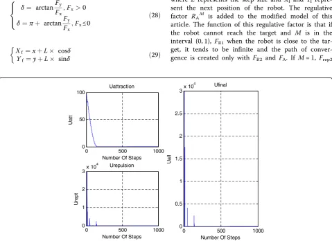
δ¼ arctanFy

where L represents the step size and Xf and Yf

repre-sent the next position of the robot. The regulative

factor RAM is added to the modified model of this

article. The function of this regulative factor is that if

the robot cannot reach the target and M is in the

interval (0, 1), FR1 when the robot is close to the tar-get, it tends to be infinite and the path of conver-gence is created only with FR2 and FA. If M= 1, Frep2

Fig. 11The simulation result of the modified artificial potential field algorithm for circular obstacles with radiusR= 0.18

0 500 1000

(10)

tends to be constant and FR1 will be zero, and the

path of convergence will be created only with FR2 and

FA. If M= 0, FR1 and FR2 will all tend to be zero, and the path of convergence will be created only by

at-traction. In the final state, generally, if M is a real

positive number, the robot does not face the local minimum cases or the inaccessibility of the target.

4 Simulation results and analysis

In this section, a comparison is firstly done between the simulation results of the artificial potential field algo-rithm and the modified artificial potential field, then the obstacle avoidance of the mobile robot is displayed against a variety of obstacles that are simulated using the modified artificial potential field algorithm.

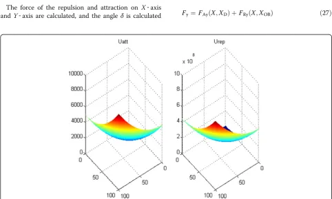
Fig. 13Mesh plot of the potential energy of attraction and repulsion in the modified artificial potential field algorithm for circular obstacles with radiusR= 0.18

0 50 100 150

0 20 40 60 80 100 120

X

Y

start point

target point

(11)

In the artificial potential field algorithm in which its relation was said in Section2, if the value to the param-eter be considered asZ= 100, M= 2, kS= 1.1, G0= 0.11, and L= 0.1 and obstacles on a circle of the radius R= 0.18, the result is as shown in Fig.8; the robot is trapped and stands at the local minimum. Figure 9 shows that the repulsive force is more than the attraction at all stages, which means the robot is trapped at the local

minimum. If these parameters are changed to any de-sired extent other than these values, there will be no change to the status of the robot at the local minimum. The mesh plot of this simulation as shown in Fig.10. It describes the obstacles like summit, target act cavity and absorb the robot inside itself.

In the modified artificial potential field algorithm in which its relation was said in Section3, if the value to the

0 5000 10000

0 5000 10000 15000

Number Of Steps

Ua

tt

Uattraction

0 5000 10000

0 200 400 600 800

Number Of Steps

Ure

p

t

Urepulsion

0 5000 10000

0 5000 10000 15000

Number Of Steps

Ua

ll

Ufinal

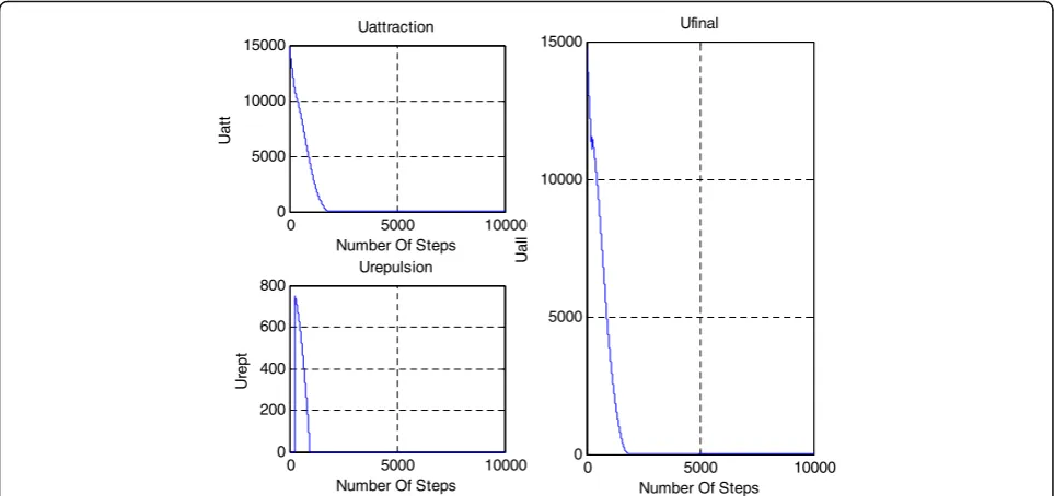
Fig. 15The energy amount of repulsion and attraction and their yields according to the number of steps in the modified artificial potential field algorithm for circular obstacle with radiusR= 30

(12)

parameter be considered asZ= 100, M= 2,kS= 1.1,G0= 0.11, andL= 0.1 and obstacles on a circle of the radiusR

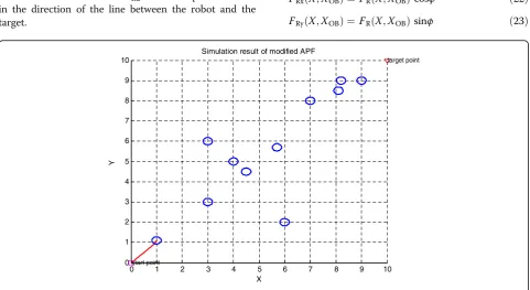
= 0.18, the result is as shown in Fig. 11. By comparing Figs.8and11, it can be seen that in the artificial potential field algorithm, the robot cannot reach the target and is trapped in a local minimum, but with the same condi-tions, in the modified artificial potential field algorithm, it achieves the target by avoiding obstacles.

Figure 12 shows that with the number of steps of

nearly 200 rounds, the attraction force is zeroed; that means, with this number of steps, the robot reaches the target. The mesh plot of this simulation in Fig.13shows that the obstacles like the summit and the target act like the cavity and absorb the robot into itself.

In the modified artificial potential field algorithm in which its relation was said in Section 3, if the value to

0 20 40 60 80 100 120 140 160 180 200

Fig. 17The result of simulating circular obstacles with radiusR= 7 in the modified artificial potential field algorithm

0 500 1000

(13)

the parameter be considered asZ= 100, M= 2, kS= 1.1,

G0= 5, andL= 0.1 and obstacles on a circle of the radius

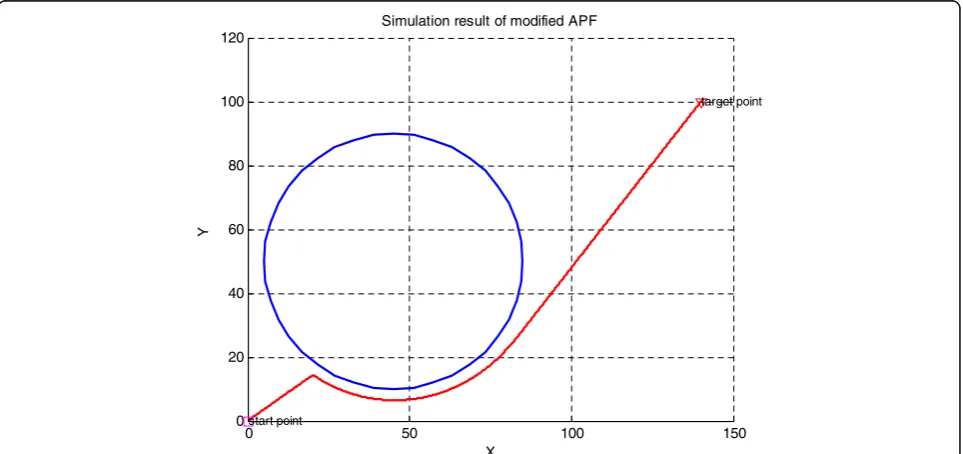
R= 40, the result is as shown in Fig. 14. It shows that the robot achieves the target by avoiding obstacles.

nearly 400 rounds, the attraction force is zeroed; that means, with this number of steps, the robot reaches the target. The mesh plot of this simulation in Fig.16shows

that the obstacles like the summit and the target act like the cavity and absorb the robot into itself.

In the modified artificial potential field algorithm in which its relation was said in Section 3, if the value to the parameter be considered as Z= 100, M= 2, kS= 1.1,

G0= 2.1, andL= 0.5 and obstacles on a circle of the ra-diusR= 7, the result is as shown in Fig.17. It shows that the robot achieves the target by avoiding obstacles.

Fig. 19Mesh plot of the potential energy of attraction and repulsion in the modified artificial potential field algorithm for circular obstacles with radiusR= 7

0 1 2 3 4 5 6 7 8 9 10

X

Y

start point

target point

(14)

Figure 18 shows that with the number of steps of nearly 700 rounds, the attraction force is zeroed; that means, with this number of steps, the robot reaches the target. The mesh plot of this simulation in Fig. 19 shows that the obstacles like the summit and the tar-get act like the cavity and absorb the robot into itself.

In the modified artificial potential field algorithm in which its relation was said in Section 3, if the value to the parameter be. considered as Z= 100, M

= 2, kS= 1.1, G0= 0.2, and L= 0.03 and the obstacle is considered as Y¼ ð_X1Þ2þ0:5;X∈ð0:7;3:5Þ , the result is as shown in Fig. 20. It shows that the robot achieves the target by avoiding obstacles.

0 500 1000 1500 0

50 100 150

Number Of Steps

Ua

tt

Uattraction

0 500 1000 1500 0

2 4 6x 10

4

Number Of Steps

Ure

p

t

Urepulsion

0 500 1000 1500 0

1 2 3 4 5 6x 10

4

Number Of Steps

Ua

ll

Ufinal

Fig. 21The energy amount of repulsion and attraction and their yields according to the number of steps in the modified artificial potential field algorithm for the curve-shaped obstacle

(15)

Figure 21 shows that with the number of steps of nearly 1000 rounds, the attraction force is zeroed; that means, with this number of steps, the robot reaches the target. The mesh plot of this simulation in Fig.22shows that the obstacles like the summit and the target act like the cavity and absorb the robot into itself.

In the modified artificial potential field algorithm in which its relation was said in Section 3, if the value to

the parameter be considered as Z= 100, M= 2, kS= 1.1,

G0= 0.3, andL= 0.1 and the obstacle is considered asX

= 4; 4≤Y≤7, the result is as shown in Fig.23. It shows that the robot achieves the target by avoiding obstacles.

nearly 900 rounds, the attraction force is zeroed; that means, with this number of steps, the robot reaches the target. The mesh plot of this simulation

0 1 2 3 4 5 6 7 8 9 10

Fig. 23The result of the straight line obstacle simulation in the modified artificial potential field algorithm

0 500 1000

(16)

in Fig. 25 shows that the obstacles like the summit and the target act like the cavity and absorb the robot into itself.

In the modified artificial potential field algorithm in which its relation was said in Section 3, if the value to the parameter be considered as Z= 100, M= 2, kS= 1.1,

G0= 0.2, and L= 0.03 and the obstacle is considered as

Y= 4; 4≤X≤6 andx= 4; 3≤y≤4, the result is as shown

in Fig.26. It shows that the robot achieves the target by avoiding obstacles.

nearly 700 rounds, the attraction force is zeroed; that means, with this number of steps, the robot reaches the target. The mesh plot of this simulation in Fig.28shows that the obstacles like the summit and the target act like the cavity and absorb the robot into itself.

Fig. 25Mesh plot of the potential energy of attraction and repulsion in the modified artificial potential field algorithm for the straight line obstacle

0 1 2 3 4 5 6 7 8 9 10

start point

target point

(17)

5 Conclusion

In this paper, improvement of the artificial potential field algorithm has been evaluated. If any obstacles are around the target, it allows the robot to find a safe path, move without collision with the obstacle, and not trapped at the local minimum then reach the target

point. The artificial potential field is a relatively mature algorithm that is widely used for its math calculations. However, due to the local minimum problem in this al-gorithm, the robot cannot achieve the target, so in order to solve this problem, a new method is proposed in this paper to remedy this algorithm. The proposed method is

0 500 1000

0 50 100 150

Number Of Steps

Ua

tt

Uattraction

0 500 1000

0 5 10x 10

284

Number Of Steps

Ure

p

t

Urepulsion

0 500 1000

0 1 2 3 4 5 6 7 8 9x 10

284

Number Of Steps

Ua

ll

Ufinal

Fig. 27The energy amount of repulsion and attraction and their yields according to the number of steps in the modified artificial potential field algorithm for the broken line obstacle

(18)

simulated in the MATLAB environment. The results of simulation evaluations show that in the modified artifi-cial potential field algorithm, the robot can pass obsta-cles around the target without collision and reach the target.

Abbreviations

APF:Artificial potential field; MSD: Mobile sensor deployment; MSNs: Mobile sensor networks; NCON: Network CONnectivity; SDRE: State-dependent Riccati equation; TCOV: Target COVerage; VHF: Vector histogram field

Acknowledgements

Authors of this would like to express the sincere thanks to the National Natural Science Foundation of China for their funding support to carry out this project.

Funding

This work is supported by the National Natural Science Foundation of China (61772454, 6171171570).

Availability of data and materials

The data is available on request with prior concern to the first author of this paper.

Authors’contributions

All the authors conceived the idea, developed the method, and conducted the experiment. SMHR contributed to the formulation of methodology and experiments. AKS contributed to the data analysis and performance analysis. JW contributed to the overview of the proposed approach and decision analysis. XL contributed to the algorithm design and data sources. All authors read and approved the final manuscript.

Authors’information

Nil

Ethics approval and consent to participate

All the authors of this manuscript would like to declare that mutually agreed no conflict of interest. All the results of this paper with respect to the experiments on human subject.

Consent for publication

Not Applicable

Competing interests

The authors declare that they have no competing interests.

Publisher’s Note

Springer Nature remains neutral with regard to jurisdictional claims in published maps and institutional affiliations.

Author details

1

Department of Electrical and Computer Engineering, Shiraz University of Technology, Shiraz, Iran.2_{School of Computing Science and Engineering,}

Vellore Institute of Technology (VIT), Vellore 632014, India.3School of Computer & Communication Engineering, Changsha University of Science & Technology, Changsha, China.4School of Automation, Wuhan University of Technology, Wuhan 430070, China.

Received: 19 December 2018 Accepted: 5 March 2019

References

1. I.R. Nourhakhsh, R. Siegwart,Introduction to autonomous mobile robots(the MIT Press, Cambridge, 2004), pp. 1_–321.

2. G. Han, C. Zhang, J. Jiang, X. Yang, M. Guizani,“Mobile Anchor Nodes Path Planning Algorithms using Network-density-based Clustering in Wireless Sensor Networks”. J. Netw. Comput. Appl.18, 1–26 (2016).

3. S. Hacohen, S. Shoval, N. Shvalbc, Applying probability navigation function in dynamic uncertain environments. Robot. Auton. Syst.87, 237–246 (2017).

4. S. Herzog, F. Wörgötter, T. Kulvicius,“Generation of movements with boundary conditions based on optimal control theory_”. Robot. Auton. Syst.

94, 1–33 (2017).

5. A. Yufka, O. Parlaktuna, inProceedings of the 5th International Advanced Technologies Symposium, International Advanced Technologies Symposium. Performance comparison of bug algorithms for mobile robots (2009), pp. 1_–5.

6. O. Khatib, Real-time obstacle avoidance for manipulators and mobile robots. Int. J. Robot. Res., 90–98 (1986).

7. J. Borenstein, Y. Koren, The vector field histogram-fast obstacle avoidance for mobile robots. IEEE Trans. Robot. Autom.7, 278–288 (1991). 8. Kushnerik AA., Vorontsov AV., Scherbatyuk APh.,“Small AUV docking

algorithm near dock unit based on visual data”, 0-933957-38-1/09, 2009. 9. H.P. Moravec, Sensors fusion in certainty grids for mobile robots. AI Mag.

9(2), 61 (1988).

10. V. Sezer, M. Gokasan, A novel obstacle avoidance algorithm:“Follow the Gap Method_”. Robot. Auton. Syst.60, 1123_–1134 (2012).

11. M.C. Fang, S.M. Wang, M.C. Wua, Y.H. Lin, Applying the self-tuning fuzzy control with the image detection technique on the obstacle-avoidance for autonomous underwater vehicles. Ocean Eng.93, 11_–24 (2015). 12. Y. Chen, H. Peng, J. Grizzle,“Obstacle Avoidance for Low-Speed

Autonomous Vehicles With Obstacle Function”. IEEE Trans. Control Syst. Technol.26, 1–13 (2018).

13. M.G. Plessen, D. Bernardini, H. Esen, A. Bemporad,“Spatial-Based Predictive Control and Geometric Corridor Planning for Adaptive Cruise Control Coupled With Obstacle Avoidance”. IEEE Trans. Control Syst. Technol.26, 1– 13 (2018).

14. D. Han, H. Nie, J. Chen, M. Chen, Dynamic obstacle avoidance for manipulators using distance calculation and discrete detection. Robot. Comput. Integr. Manuf.49, 98_–104 (2018).

15. M. Mendes, A.P. Coimbray, M.M. Crisostomoy,_“Assis - Cicerone Robot With Visual Obstacle Avoidance Using a Stack of Odometric Data”. IAENG Int. J. Comput. Sci.45, 1_–9 (2018).

16. P.D.H. Nguyen, C.T. Recchiuto, A. Sgorbissa,_“Real-time path generation and obstacle avoidance for multirotors: a novel approach”. J. Intell. Robot. Syst.

89, 1_–23 (2017).

17. A. Behboodi, S.M. Salehi,“SDRE controller for motion design of cable-suspended robot with uncertainties and moving obstacles”. Mater. Sci. Eng.

248, 1–6 (2017).

18. Y. Liu, D. Chen, S. Zhang, in3rd International Conference on Control and Robotics Engineering. Obstacle Avoidance Method Based on the Movement Trend of Dynamic Obstacles (2018), pp. 45–50.

19. M. Odelga, P. Stegagno, N. Kochanek, H.H. Bülthoff, inIEEE International Conference on Robotics and Automation. A Self-contained Teleoperated Quadrotor: On-board State-Estimation and Indoor Obstacle Avoidance (2018), pp. 7840_–7847.

20. P.D. H. Nguyen, C.T. Recchiuto, A. Sgorbissa,_“Real-time path generation and obstacle avoidance for multirotors: a novel approach”. J. Intell. Robot. Syst.

89, 27_–49 (2017).

21. X. Li, S. Song, Y. Guo,_“Robust finite-time tracking control for Euler_–Lagrange systems with obstacle avoidance”. Nonlinear Dyn.93, 1–9 (2018). 22. Z. Liao, J. Wang, S. Zhang, J. Cao, G. Min, inIEEE Transactions on Parallel and

distributed systems. Minimizing Movement for Target Coverage and Network connectivity in Mobile Sensor Networks (2014), pp. 1–14.

23. B. Alkandari, K. Pahlavan, inIEEE 25th_{Internatinal Symposium on Personal,}

Indoor and Mobile Radio Communications. Performance Bounds of Multi-Relay Deployment of Wireless Data Networks (2014), pp. 1541_–1546. 24. S. Xie, P. Wu, Y. Peng, J. Luo, D. Qu, Q. Li, J. Gu, in2014 IEEE

International Conference on Information and Automation. The obstacle avoidance planning of USV based on improved artificial potential field (2014), pp. 746–751.

25. T.T. Mac, C. Copot, A. Hernandez, R.D. Keyser, inIEEE 14th International Symposium on Applied Machine Intelligence and Informatics. Improved Potential Field Method for Unknown Obstacle Avoidance Using UAV in Indoor Environment (2016), pp. 345_–350.

26. Q. Zhu, Y. Yan, Z. Xing, inIEEE Sixth International Conference on Intelligent Systems Design and Applications, China. Robot Path Planning Based on Artificial Potential Field Approach with Simulated Annealing (2006), pp. 1–6.

(19)

Large-Scale Spacecraft Swarm Using Artificial Potential Field and Bifurcation Dynamics (2018), pp. 1_–26.

28. A. Nikranjbar, M. Haidari, A.A. Atai, inIEEE Sixth International Conference on Intelligent Systems Design and Applications, China. Adaptive Sliding Mode Tracking Control of Mobile Robot in Dynamic Environment Using Artificial Potential Fields (2018), pp. 1_–6.

29. F.A. Raheem, M.M. Badr,“Development of Modified Path Planning Algorithm Using Artificial Potential Field (APF) Based on PSO for Factors Optimization”, American Scientific Research Journal for Engineering, Technology, and Sciences.37, 316_–328 (2018).

30. S.M.H. Rostami, A.K. Sangaiah, J. Wang, H.J. Kim, Real-time obstacle avoidance of mobile robots using statedependent Riccati equation approach. EURASIP J. Image Video Process, 1–13 (2018).

31. S.M.H. Rostami, M. Ghazaani, State dependent Riccati equation tracking control for a two link robot. J. Comput. Theor. Nanosci.15, 1490–1494 (2018).

32. S.M.H. Rostami, M. Ghazaani,“Design of a fuzzy controller for magnetic levitation and compared with proportional integral derivative controller_”. J. Comput. Theor. Nanosci.15, 3118–3125 (2018).

33. S.M.H. Rostami, M. Ghazaani,“An intelligent power control design for a wind turbine in different wind zones using FAST simulator. J. Comput. Theor. Nanosci.16, 25_–38 (2019).

34. F.A. Raheem, M.M. Badr, Obstacle avoidance control of a human-in-the-loop mobile robot system using harmonic potential fields. Robotica, 1–21 (2017). 35. R. Zhu, X. Zhang, X. Liu, W. Shu, T. Mao, B. Jalaeian, ERDT: Energy-efficient

reliable decision transmission for cooperative spectrum sensing in industrial IoT. IEEE Access3, 2366–2378 (2015).

36. H. Samani, R. Zhu, Robotic automated external defibrillator ambulance for emergency medical service in smart cities. IEEE Access4, 268–283 (2016). 37. G. Fedele, L. D_’Alfonso, F. Chiaravalloti, G. D_’Aquila, Obstacles avoidance

based on switching potential functions. J. Intell. Robot. Syst.90, 387–405 (2018).