R E S E A R C H
Open Access
Optimizing radio resources for
multicasting on high-altitude platforms
Ahmed Ibrahim
1,2 *and Attahiru S. Alfa
1,3Abstract
High-altitude platforms (HAPs) are quasi-stationary aerial wireless communications platforms meant to be located in the stratosphere, to provide wireless communications and broadband services. They have the ability to fly on demand to temporarily or permanently serve regions with unavailable infrastructure. In this paper, we consider the
development of an efficient method for resource allocation and controlling user admissions to multicast groups in a HAP system. Power, frequency, space and time domains are considered in the problem. The combination of these many aspects of the problem in multicasting over an OFDMA HAP system were not, to the best of our knowledge, addressed before. Due to the strong dependence of the total number of users that could join different multicast groups on the possible ways we may allocate resources to the different multicast groups, it is important to consider a joint user to multicast group assignments and radio resource management across the groups. From the service provider’s point of view, it would be in its best interest to be able to admit as many users as possible, while satisfying their quality of service requirements.
The problem turns out to be a mixed integer non-convex non-linear program for which branch and bound solution framework is guaranteed to solve the problem. Branch and bound (BnB) can be also used to obtain sub-optimal solutions with desired quality. Even though branch and bound is guaranteed to find the optimal solution, the computational cost could be extremely high, which is why we considered different types of enhancements to BnB. Mainly, we consider reformulations by linearizing a specific set of quadratic constraints in the derived formulation, as well as the application of different branching techniques to find the one that performs the best. Based on the conducted numerical experiments, it was concluded that linearization, applied for at least 100 presolving rounds, and cloud branching achieve the best performance.
Keywords: High-altitude platforms, Radio resource allocation, Multicasting, Admission control, Optimization
1 Introduction to high-altitude platforms
Delivering high-capacity services over wireless medium presents challenges, since the spectrum is limited and the demand for its access is constantly growing. For terrestrial cellular networks, the solution is to decrease the transmis-sion range of a base station (BS) and deploy more base stations which require backhaul interconnections. Clearly, this is a costly and difficult proposition, especially for areas with hostile geographical nature. This pressure on the radio spectrum requires moving higher in frequency
*Correspondence:[email protected]
1Department of Electrical and Computer Engineering, University of Manitoba, Winnipeg MB, R3T 5V6, Canada
2Faculty of Engineering and Applied Sciences Memorial University of Newfoundland, St. John’s NL, A1B 3X5, Canada
Full list of author information is available at the end of the article
to K/Ka bands (26–40 Ghz), which are less heavily con-gested and can provide significant bandwidth. The main problem with working in K/Ka bands is that line-of-sight
(LOS) or quasi-LOS propagation is needed [1].
The visibility problem can be solved using satellite tech-nology, which is a well-established alternative to terres-trial infrastructures that is able to serve wide areas with a cellular coverage, thus implementing frequency reuse
paradigms. Geostationary Earth orbit (GEOs) satellites
are located at about 36 thousand kilometers away from the earth’s surface. Due to the large distance from the earth’s surface, GEOs have huge antenna footprints that can cover entire continents providing services to millions of users. However, being far away from the earth’s sur-face also has major drawbacks, mainly due to the very critical free-space path loss and large propagation delays.
The solution to these problems require large antennas and sophisticated architectures and protocols at the cus-tomer receivers. Furthermore, technological constraints for on-board antennas prevent the possibility of optimiz-ing the cell dimension on the ground, thus potentially lowering frequency reuse efficiency and, consequently,
overall capacity. Another type of satellites is theLow Earth
Orbit(LEO) satellites which overcomes many of the draw-backs specific to GEO satellites as they are much nearer to the earth’s surface (200–1600 km). However, a single LEO satellite based system would not be suitable for real-time transmission since the satellite is frequently out of visibility. In such a system, only store and forward tech-niques could be used. If continuous coverage is required, then an entire constellation of LEO satellites must be used. Obviously this is too costly, and necessitates that efficient handover schemes be used among the satellites.
A potential solution for these problems that has been adopted is carrying communications relay payloads and operating in a quasi-stationary position in the strato-sphere layer of the atmostrato-sphere. LOS propagation paths can be provided to most users, with modest free space path loss and propagation delays, thus enabling services that take advantage of the best features of both wireless terrestrial and satellite communications. The platforms
that carry these payloads were calledhigh-altitude
plat-forms(HAPs) [2].
HAPs are quasi-stationary aerial platforms that are meant to be located at a height of 17–22 km above earth’s surface in the stratosphere layer. Many of their pros are a combination of those in both, terrestrial wireless and satellite communication systems. Some of those pros are [3]:
• Their ability to fly on demand to temporarily or permanently serve regions with unavailable telecommunications infrastructure.
• A single HAP has a large area coverage that can go up to 150 km compared to a single terrestrial cellular base station (BS) whose maximum radius, for macro cells, is in the range of 20–30 km.
• Low propagation delays compared to satellites which implies better perceived quality of service (QoS) by the users for real-time applications like voice and video.
• Stronger received signal strengths as compared to satellites and hence user terminals need not be bulky. • Deployment time is low since one platform and
ground support are sufficient to start the service. • Much less ground-based infrastructure compared to
terrestrial cellular networks.
For the same allocated bandwidth in a specified area, ter-restrial systems require a large number of base stations. On the other hand, GEO satellites have cell size limitations
due to large footprints on the earth’s surface and non-geostationary satellites face handover problems and the need to deploy the entire constellation , thus requiring high launching costs to place them in orbits. In this case, HAPs seem to be an attractive choice.
2 Recent works in HAPs
Among the recent works in the area of HAPs, is the
work done by Sudheesh et al. in [4]. In their paper, they
show how spatial multiplexing could be performed to boost the spectral efficiency. They state that in a sin-gle HAP system with multiple antennas on-board, spatial multiplexing cannot typically be achieved due to high cor-relation between paths. Therefore, they proposed the use of multiple spatially separated HAPs to perform precise beamforming. Due to the high altitudes and imperfect stabilization, it is challenging to acquire accurate chan-nel state information (CSI), that is necessary for precise beamforming. For this, the authors realize an interfer-ence alignment technique based on a multiple antenna tethered balloon that could be deployed and used as a relay between the multiple HAPs and the ground stations. In particular, a multiple-input multiple-output X network
was considered in [4], and the capacity for that network
was obtained in close form. The authors showed that a maximum sum-rate was obtained.
In [5], Xu et al. proposed a geometry based HAP channel
model that considers the statistical and geometry prop-erties of terrestrial environments comprehensively for the purpose of efficient deployment of HAPs. Based on their proposed channel model, they also derived the LOS trans-mission probability of air-to-ground communication and performed the analysis for the path loss. They also pro-posed an algorithm that maximizes the efficiency, in terms of the ratio of the radius of HAP footprint to inter-HAP
distance. In [6], Dong et al. treated HAPs as mobile base
stations and considered a method for their placement with guarantees on QoS and user demands in a constellation of multiple interconnected HAPs. They established QoS metrics by considering the information isolation, integrity, rate and availability. The user demand has been modeled by considering the broadband size, the population distri-bution density, and scale factor of the HAP network users. Based on the network coverage model, they gave out the design vector of HAPs layout optimization, i.e., number of HAPs, downlink antenna area, power of payload,
lon-gitude of HAP and latitude of HAP. Moreover, in [6] a
nonlinear, nonconvex, and non-continuous combinatorial optimization model was proposed. This was solved by an improved artificial immune algorithm.
In [7], Zhang et al. considered UAV-enabled mobile
link blocked. In their paper, they study two problems, spectrum efficiency and energy efficiency maximization for that system and revealed their trade-off with the UAV’s propulsion energy taken into account. The type of motion that they considered is circular, and the type of relaying is a decode and forward in a time-division duplex mode. They derived the optimal solutions for both problems and showed that energy efficiency maximization requires a larger circular trajectory radius than spectral efficiency maximization. Their numerical results showed perfor-mance gain for mobile relay in circular trajectory over static relaying with a fixed relay.
In [8], the design of an active electronically steerable
antenna array (AESA) enabling broadband line-of-sight communication from HAPs was investigated. The array is constructed using a multitude of single chip multi-channel beamforming modules capable of switched bi-directional amplitude and phase conditioning at Ka-band enabling sharing of aperture between transmitting and receiving
functions. In [9], the authors describe the development
and test of an electrically steerable phased array antenna for implementation in multilayer circuit board architec-ture. The arrays were designed for use in HAPs demon-strations to support RF links to mechanically steered user terminals. They achieved measured performance results for K-band 256 element receive arrays.
A very recent survey [10] on airborne communications
(ACNs) provides a perspective on general procedures of designing ACNs, including HAPs. The paper surveyed primary mechanisms and protocols for the design of ACNs concerning low altitude platforms, high-altitude platforms and integrated ACNs. It discussed specific char-acteristics such as highly dynamic network topologies, high network heterogeneity, weakly connected communi-cation links, complex radio frequency (RF) propagation model, and platform constraints (e.g., size, weight and power) in ACNs. The authors of the paper emphasized that these three areas are building blocks for the architec-ture of ACNs. This architecarchitec-ture fastens together with a broad range of technologies from control, networking and transmissions.
3 Radio resource allocation and admission control for multicasting in HAPs (Methods) There are many aspects involved in wireless communication
networks that have an impact on performance [11–13].
Just like any wireless network, one of these crucial issues is that a HAP needs to manage its radio resources as efficiently as possible in order to gain the maximum desired benefit. This benefit could be the system data capacity, number of users that could be served in the sys-tem, throughput fairness among the system’s users, packet
losses etc. One of the aspects thatradio resource
alloca-tion(RRA) has a direct impact on is the admission of users
in the system. Simply, the availability of resources deter-mines how many users can be admitted, or served in the system. The radio resources that need to be managed for a
HAP having multiple antennas usingorthogonal frequency
division multiple access(OFDMA) are the following:
1. The radio power
2. The frequency subchannels
3. The time slots over the subchannels 4. The antennas (antenna selection)
Choosing which users to admit into the system affects the total number admitted. This is because the users have different channel conditions due to their different posi-tions and also due to the random nature of the radio channel. For example, if a user is in a location where the received signal quality is poor, and it is to be admitted into the system, it would need considerable radio power to compensate for the channel attenuation. This could lead to little remaining power that is insufficient to admit other users. If that user would have not been admitted, the HAP might have been able to serve a larger number of users with good channel conditions. This is a simple example considering power only. It grows much more complex when subchannels, time slots and antenna selections are to be allocated too.
Multicasting is the transmission of the same informa-tion to a group of users instead of transmitting the same information to each user individually (unicasting). This type of transmission saves a lot of radio resources as com-pared to unicasting, and is therefore, usually the method used to transmit same information to a group of users in any network. We can have more than one multicasting session in a HAP system and each user may want to join more than one session at the same time. Each multicast session transmits its data on the same set of subchannels, time slots, and antennas with the same power level for all
users in the multicast group. RRA is needed foradmission
control(AC) of multicast sessions so that efficient admis-sion deciadmis-sions are made for users wishing to join different multicasting groups.
Since aeronautically reliable platforms and their flight regulations are still in the development phase, the amount of published research for telecommunication services over HAPs, particularly RRA and AC, is limited compared to other wireless systems, let alone RRA and AC for multicasting in specific. Moreover, most of the big re-search projects for HAP like SHARP, Skynet, StratSat,
HALO,CAPANINA, Helinet, and HAPCOS [14–19]
star-ted their activities between 2000-2006, a time in which the most popular wireless interface in wireless
telecom-munications research was code division multiple access
(CDMA) based Universal Mobile Telecommunications
Orthogonal Frequency Division Multiplexing (OFDM) is one of the possible techniques to be used for transmis-sion between the HAP and the users due to its well known capabilities in mitigating wireless channel impair-ments that result from high mobility and high
transmis-sion speeds [20]. Hence, the multiple access scheme that
is expected to be used in HAPs is OFDMA. Therefore, we believe that more research in HAPs should be done considering this type of interface.
3.1 Differences between rRA in HAP systems and terrestrial cellular systems
RRA over a multicellular HAP system differs from con-ventional terrestrial cellular systems mainly due to an inherent graceful high centralization in the HAP. In the downlink, there is one common source of RF power for all the cells of a given HAP, while for a group of con-tiguous cells of a terrestrial cellular system, each cell has a separate BS each with independent RF power source. The same is true for the spectrum, where for the HAP the entire spectrum is shared among the HAP’s cells while in conventional terrestrial cellular systems every cell uses a portion of the spectrum, depending on the frequency reuse pattern, to minimize inter-cell interference.
Also, a single HAP has the ability to have global knowl-edge of the channel gains of the users in all its cells at all subchannels. This is possible since all users in the HAP service area acquire CSI with just one transmitting entity, which is the HAP. On the other hand for terrestrial cellular systems, CSI is acquired by the users in each cell with that cell’s BS only. Therefore, for global CSI to be achieved at all BSs, a broadcast transmission for each BS’s CSI over its backhaul links would be required. This is a lot of overhead signaling that would burden the network and is hence not usually performed, leading to suboptimality in multicellu-lar RRA of terrestrial cellumulticellu-lar systems. Furthermore, the time needed to exchange information until global CSI is achieved for a given region of a terrestrial cellular system is not guaranteed to facilitate dynamic multicellular RRA at a frame by frame basis before the CSI information at each terrestrial BS change.
A HAP can thus use the global CSI information it has about all users, and the fact that it has one common power and spectrum source, to centrally perform more flexible radio allocations at the HAP with full awareness of the inter-cell interference levels instantaneously on a dynamic frame by frame basis. Conventional terrestrial cellular systems either would perform RRA locally at a single cell level, or if multicellular RRA is desired a dis-tributed approach with heavy exchange of CSI would be needed.
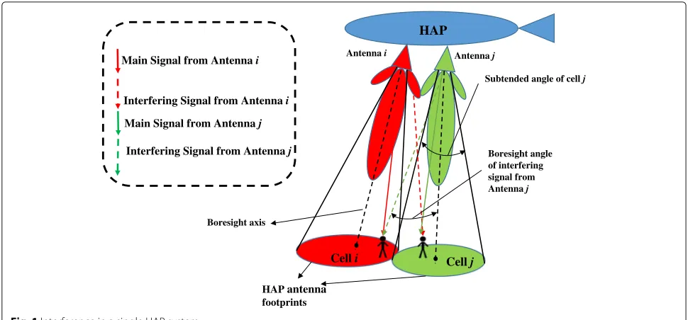
Finally, the beams of the antennas co-located on the
HAP interfere with each other, as illustrated in Fig. 1
for a single HAP system. The interference to a user in
a particular cell is due to the reception of unwanted transmissions at boresight angles greater than angles that subtend the neighbor cell footprints through the main-lobes and side main-lobes of their antennas [21]. The collocation of the antennas allows the HAP to centrally perform electronic cell resizing by controlling the antenna beam-widths and pointing angles in an RRA problem, depending on the user distribution and/or density in a given cell, to dynamically control co-cell interference. This is not read-ily possible in conventional terrestrial cellular systems.
3.2 Motivations for the proposed aC-RRA scheme This paper studies and proposes a novel admission con-trol and radio resource allocation scheme for a single HAP system with antennas on-board. Derivations for the mathematical formulations are done and suitable problem specific and structure oriented solution methodologies are used. The problem considered in this paper is joint AC-RRA for an OFDMA based HAP system with mul-tiple multicasting sessions of heterogenous priorities at each user, in the downlink. The users have heteroge-neous priorities from the service provider point of view. The QoS requirements of the admitted users and their associated multicast groups’ requirements must be met, or they should not be admitted in the first place. The QoS requirements considered in this paper are the signal-to-interference-noise-ratio (SINR) of a multicast session for each user and the session’s minimum and maximum data capacity constraints for all the multicast groups. In
our earlier works in [22–24], we considered maximizing
the spectrum utilization by serving the largest number of users on all the available frequency-time slots. In the extended problem in this paper, we consider maximizing the number of highest priority users admissions, to their most favored sessions each.
We briefly highlight the differences between the
sys-tem model we had in our earlier works [22–24] and an
extended one that we consider in this paper. From now on, we will be referring to the system model in [22–24] as the primary problem (P-Prob), in which:
1. The concept of “cells” was adopted where each user falling within the foot print of antenna beam is associated with that antenna only. Hence, a user can only receive from one antenna at most and any possible antenna beam overlaps are not exploited. 2. A user can request, and hence can only receive
sessions being transmitted in the cell in which the user resides.
3. All users assumed the same level of priority to the service provider, and all the sessions a given user requested were all of equal importance.
HAP
Cell i Cell j
Antenna i Antenna j
Main Signal from Antenna i
Interfering Signal from Antenna i
Main Signal from Antenna j
Interfering Signal from Antenna j
Boresight axis
HAP antenna
footprints
Boresight angle of interfering signal from Antenna j
Subtended angle of cell j
Fig. 1Interference in a single HAP system
The extended problem (E-Prob), which this paper focuses on, considers the following:
1. More flexibility by allowing transmission of a multicast session to the users in a group on more than one antenna simultaneously given an acceptable level of SINR is met for all users in the group. 2. A user can request, and hence receive, sessions being
transmitted in any overlapped adjacent cell of the HAP service area, hence exploiting the possible antenna beam overlaps.
3. Each user is assumed to have heterogeneous priority levels for different multicast sessions. Also from the service provider’s point of view, the user priorities could be heterogeneous.
4. The objective is to maximize the total number of admitted users with highest priorities, each to the sessions of highest priority to the user.
P-Prob was the first part of our research work that was
published in [22–24]. Since that problem was very rich
and considered many different aspects that were not con-sidered together, by other researchers in previous works for HAPs (to the best of our knowledge), we decide to go deeper in the same problem after including the extensions mentioned above to see if we could achieve an improve-ment. Since there could be many ways to formulate the same problem, we preferred to try to find a formulation that could be solved more efficiently than the one we
obtained for P-Prob in [24]. We were successful in
obtain-ing a much smaller formulation which we believe is an important achievement as any algorithm’s computational effort is always function in the formulated problem size, for the same problem class.
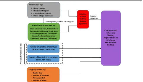
Formulating the problem using much smaller number of variables and constraints is an important step to reduce the computational effort and memory requirements by
the HAP computing hardware on-board. Figure2shows
all the different aspects that contribute to the compu-tational effort and memory requirements of solving an optimization problem for multicasting joint AC-RRA. As we show in the figure in a general sense, the key factors of a formulation are the problem’s type (e.g., linear, integer, mixed integer liner), and the presence of any special structure (e.g., knapsack, transportation, quadratic, convex), the most suitable algorithm (e.g., dynamic programming, Dijktra’s algorithm, feasible direc-tions method, branch and bound) in terms computational
efficiency can be determined. Also, as Fig.2shows, any
algorithm’s complexity is function in the problem size fed to it, and the relative numbers of different types of variables and constraints. When we have integer and continuous variables, the impact of integer variables on the computational effort is much stronger as compared to the continuous variables. The same saying goes for nonlinear constraints versus linear constraints. Therefore,
since our earlier formulation for P-Prob in [22–24] has
a huge number of binary variables and non-linear con-straints, the huge reduction in their numbers that we achieve in this paper for E-Prob would have crucial impact on the computational complexity encountered in solving the problem.
Since we are able to greatly reduce the problem size, we are able to extend the system model (to E-Prob) while still having a far much smaller formulation than that we
obtained and solved for in P-Prob in [24]. Hence the
Fig. 2Illustration of all the factors that contribute to the computational effort and memory requirements in solving an AC-RRA optimization problem
models, P-Prob and E-Prob, is the formulation size for
each. This explained in Section7.
Other than our earlier works in [22–24], we have not
seen similar models in the HAP literature, probably due to their high complexity, which was the reason we decided to take a step in the direction of combining the following into one problem in this paper:
1. Power allocation to multicast groups 2. Subchannel allocation
3. Time scheduling
4. Multiple antenna selection
5. User to multicast group assignments 6. Heterogeneous user priorities 7. Reusing spectrum
3.3 Scope and contribution of the paper
For the derived efficient formulation for E-Prob in this paper, a branch and bound framework is proposed in which we use linear outer approximation by McCormick underestimators as a relaxation for the formulated mixed
binary quadratically constrained program [25] andmixed
integer linear programmingtechniques. Different branch-ing schemes for the branch and bound scheme are used and their performances are evaluated by numerical
exper-iments [26]. Also, a reformulation technique that
lin-earizes a certain type of quadratic constraints in the formulation is used and computational experiments are
conducted to evaluate the performance with and without the reformulation linearization scheme. Domain propa-gation methods, separating cuts and heuristics are also used in the BnB framework for solving the formulation of
E-Prob [27], but are not be discussed in this paper. For
those, we refer the reader to the first author’s thesis [28]. The parameters used for performance comparison in computational experiments are the following:
1. The duality gap
2. The number of branch and bound (BnB) nodes needed
3. The number of iterations needed
4. The average number of iterations per BnB node 5. The number of instances for which a feasible solution
is found
6. The time needed to find the first feasible solution 7. The value of the objective function
4 Multicasting in a single HAP system: an efficient formulation and an extended problem
4.1 System model
In this section, the extended system model (E-Prob), for AC-RRA for multicasting over an OFDMA based HAP system is provided. A simple standalone HAP
architec-ture [3] is considered for this paper. A user is allowed to
but also those being transmitted in neighboring cells, if the signal-to-interference-ratio is acceptable. This means that after the admission is done, a user can belong to multicast groups in different cells across the service area.
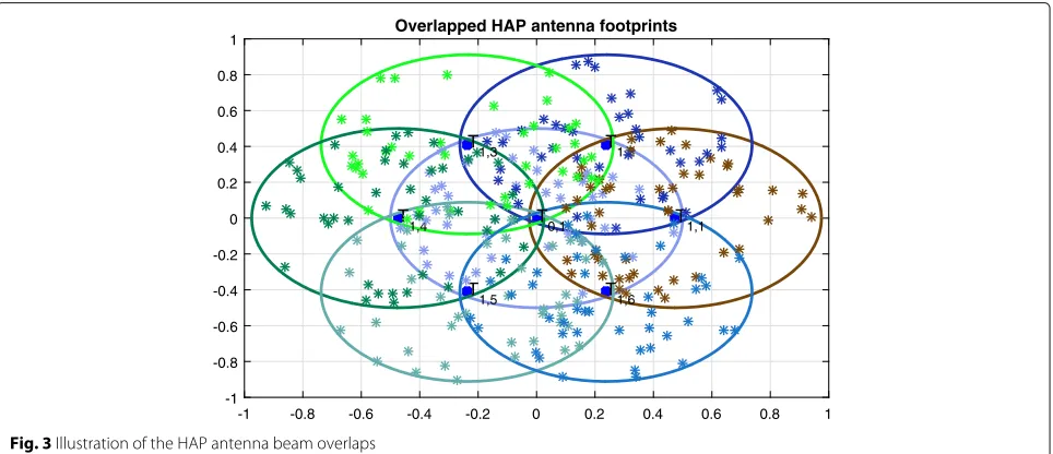
The main difference between E-Prob and P-Prob is that we no longer adopt the concept of user association to “cells” as in terrestrial cellular systems. Instead, a multi-cast group could actually receive transmission on more than one antenna on different frequency-time slots simul-taneously. P-Prob did not allow that since it adopted the concept of cells where a user can receive only from the antenna that illuminates the cell in which the user resides. In P-Prob, a group of users that receive the same multicast session in different cells were considered to be separate groups while in E-Prob, all users receiving the same mul-ticast session are considered in the same group regardless of the antennas they are receiving on. The second dif-ference is that P-Prob considered that a user can only receive multicast sessions being transmitted in the cell it resides. If a user would like to receive a session that is being transmitted in another cell but is not currently being transmitted in the cell it belongs to, they would not be able to. In E-Prob however, a user can receive a multi-cast session being transmitted in a neighboring cell, if it is not being transmitted in the cell in which the user resides in. This is possible as indicates in Fig.1, if the two
trans-missions on antennasiandjare performed on separate
sets of frequency-time slots. The possibility increases for users near the cell boundaries, especially antennas foot-prints do not have deterministic contours outside which the received power is zero and hence the received powers
from each could be overlapping in certain areas as Fig.3
shows. Finally, E-Prob considers different multicast ses-sion priorities for user-to-sesses-sion admisses-sions, where each
user could have different priority levels for the service provider, and each session has different levels of prior-ity for different users. We aim at maximizing the number of highest priority user-to-session admissions, instead of giving all the users homogeneous priority levels as in P-Prob.
The set of users that get admitted to receive a
mul-ticast session m are considered a multicast group with
the same index of the session,m. The HAP has multiple
antennas over which the multicast streams are transmit-ted to the service area. A user can request to receive more than one session and hence may be admitted to (allowed to receive) one or more of the requested sessions. This means that after the admission is done, a user can belong to more than one multicast group. Any two multicast ses-sions may not be transmitted on the same resource trio combination (i,c,t) to avoid inseparable signal
interfer-ence, where i is the antenna index, c is the subchannel
index and tis the time slot index. For a frequency-time
slot(c,t)to be assigned to a particular user to receive
ses-sion mon antenna i, it has to satisfy a minimum SINR
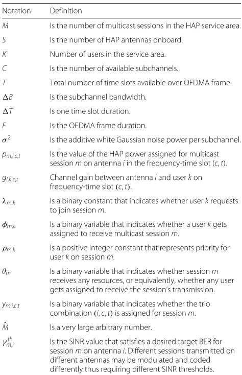
threshold γmth,i to guarantee an acceptable bit-error-rate performance.γmth,i could be different across the sessions and antennas depending on the possibly different modu-lation and channel coding schemes. The main notations used for mathematically formulating the problem, are provided in Table1.
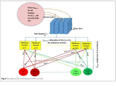
Figure 4 shows the power pm,i,c,t for session m being
assigned to the trio (i,c,t). The antenna, frequency
and time resources are represented graphically by three dimensions where the antenna dimension is not neces-sarily orthogonal to the frequency-time plane due to the possibility of antenna foot print overlaps. Orthogonal-ity here means the absence of interference between any
-1 -0.8 -0.6 -0.4 -0.2 0 0.2 0.4 0.6 0.8
-1 -0.8 -0.6 -0.4 -0.2 0 0.2 0.4 0.6 0.8 1
1 Overlapped HAP antenna footprints
T
0,1 T1,1
T 1,2 T
1,3
T 1,4
T
1,5 T1,6
Table 1Notation definitions for E-Prob formulation
Notation Definition
M Is the number of multicast sessions in the HAP service area.
S Is the number of HAP antennas onboard.
K Number of users in the service area.
C Is the number of available subchannels.
T Total number of time slots available over OFDMA frame. B Is the subchannel bandwidth.
T Is one time slot duration.
F Is the OFDMA frame duration.
σ2 Is the additive white Gaussian noise power per subchannel.
pm,i,c,t Is the value of the HAP power assigned for multicast
sessionmon antennaiin the frequency-time slot (c,t).
gi,k,c,t Channel gain between antennaiand userkon
frequency-time slot(c,t).
λm,k Is a binary constant that indicates whether userkrequests
to join sessionm.
φm,k Is a binary variable that indicates whether a userkgets
assigned to receive multicast sessionm.
ρm,k Is a positive integer constant that represents priority for
userkon sessionm.
θm Is a binary variable that indicates whether sessionm
receives any resources, or equivalently, whether any user gets assigned to receive the session’s transmission.
ym,i,c,t Is a binary variable that indicates whether the trio
combination(i,c,t)is assigned for sessionm.
ˆ
M Is a very large arbitrary number. γth
m,i Is the SINR value that satisfies a desired target BER for
sessionmon antennai. Different sessions transmitted on different antennas may be modulated and coded differently thus requiring different SINR thresholds.
pair of trios(i,c,t)represented by the small cubes in the figure. HAP power is allocated to each of the trio cubes for the different multicast sessions being transmitted to the service area. The “cubes" are assigned to the different multicast groups and the users in the HAP service area are assigned to these groups according to their priority value ρm,k,quality of service(QoS) requirements and availability of resources.
For E-Prob, there are two definitions associated with a group’s data capacity. The minimum capacity of the group is defined as:
where Bis the subchannel bandwidth,T is the time
slot duration,Fis the OFDMA frame length duration and
xm,i,k,c,teither:
• Takes the value of the SINR of the userk on the trio combination(i,c,t)if the user gets to receive session m,
• Takes a very large numberMˆ (theoretically infinity) if userk does not get to receive session m but some other users do, or
• Zero if no users in the service area are assigned to receive sessionm. an arbitrarily large number whose value is considered as infinity, andφm,k is a binary variable indicating
user-to-session admission for userk.
The channel gainsgi,k,c,tdepend upon the instantaneous values of large scale fading and small scale fading. In a HAP system, large scale fading is a result of free space path
loss and attenuation due to rain and clouds [29]. Small
scale fading is acceptably modeled as Ricean fading due to the presence of line of sight rays from the HAP to most
of the locations in the HAP service area [1]. The channel
gaingi,k,c,tbetween base station (antenna)iand userkon the frequency-time slot (c,t) can hence be given as:
gi,k,c,t=
user terminalk and antenna i boresight axis and is defined by [21]
whereApeff is the antenna’s efficiency,n is the rate of roll-off for the raised cosine function.
• dkis the distance between the HAP and user terminal
k,Cˇlightis the speed of light andfcis the carrier
frequency.
• A(dk)is the attenuation due to clouds and rain. This
depends on the distance between the HAP and each userk in the service area.
Fig. 4Illustration of the multicasting AC-RRA in E-Prob
• ϕk,c,tis the Ricean small scale gain in frequency-time
slot(c,t)for user terminalk.
We also define the maximum capacity of a multicast group as:
ˆ
Rmaxm =
S
i=1
C
c=1
T
t=1
rmmax,i,c,t, (6)
where rmaxm,i,c,t is the data capacity of session m over the trio combination(i,c,t) which is defined to be the data capacity of the user with maximum SINR on(i,c,t)and is given as:
rmaxm,i,c,t= BT F log
1+max
k tm,i,k,c,t
, (7)
wheretm,i,k,c,teither:
• Takes the value of the SINR of userk on the trio combination(i,c,t)if the user gets to receive session m, or
• Is zero if userk does not get to receive session m.
hencetm,i,k,c,tcan be expressed as:
tm,i,k,c,t=
gi,k,c,tpm,i,c,tφm,k M
m=1 ∀i=igi,k,c,tpm,i,c,t+σ2
. (8)
4.2 Key differences in the fundamental equations that describe e-Prob and p-Prob
In our earlier work in [24], since the spatial dimension was not considered (i.e., multiple antenna reception in areas of overlaps were not considered), the data rate for a multicast
groupmwas defined as:
ˆ
Rm= C
c=1
T
t=1
rminm,i,c,t (9)
which did not sum the data rates on the different antennas as Eqs. (1) and (6) do for E-Prob. This ruled out the
pos-sible advantage that users in a group in cellican receive
all the group’s users. In E-Prob, even if the group of users were to receive a session on only one antenna, the sys-tem has the flexibility to select which antenna to receive on, as long as more than one antenna stream the session. This was not permitted by the formulation (O) of P-prob in [24], that was based on equation (9). Constraint set C2
receiving sessionm and can only receive transmission from antennai,
• zm,i,k,c,tis the set of binary decision variables that
indicated whether a userk got admitted to receive transmissionm from the antenna covering cell i on a frequency-time slot(c,t),
• xm,i,c,twas a binary decision variable that indicated
whether a frequency-time slot(c,t)got assigned for the groupNm,i.
This constraint ensured that the users assigned to receive sessionmin celliover a set of frequency time slots should be the same in each of those assigned slots, since in multicasting, the same set of resources are shared by the set of users in the multicast group. The constraint at the same time enforced the set of users receiving session
min celli, to receive it from the antenna of that cell only, and treated groups receiving the same session in another cell i as a different group Nm,i. Another constraint set
in formulation (O) in [24] that did not take into account
antenna selection and possible reception from more than one antenna simultaneously, is constraint set C1 given by:
zm,i,k,c,t=
{0, 1} if λm,i,k=1,
0 otherwise, ∀m,i,k,c,t
whereλm,i,kwas a binary constant that indicated whether
userkresided in celliand sent a request to receive
ses-sion m. Since P-prob considered no cell overlaps, a user
could only physically reside in one cell and hence λm,i,k
was equal to 1 for exactly onei. This also prevented the
user from receiving transmission from any other antenna
except the one for which λm,i,k = 1, if the user got
admitted.
Note that Eq. (9) was used to impose upper and lower
data rate constraints on sessionmin cellias
Rminm ≤
that of the user with the poorest SINR. For the lower data rate constraint, this guarantees that all users in the group receive a data rate greater than the minimum. The defini-tion of a multicast group data rate in Eq. (9) was also used
to enforce a maximum rateRmaxm constraint. However, it
was noticed that the upper data rate constraint may not be necessarily satisfied for all users in a multicast group on a particular frequency-time slot if we use the data rate of the user with the poorest SINR in the group to solely describe the group’s data rate. This was the reason we introduced
rmaxm,i,c,tandRˆmaxm in Eqs. (7) and (6).
In P-Prob, the objective function was given in [24]:
max
captured the sum of the users for every multicast group
Nm,i served by each frequency-time slot(c,t) which we
define to be the spectral utilization. The objective func-tion for P-prob did not consider user-session priorities. However, for E-Prob, the next section provides the objec-tive function and interprets it, showing the difference in the objectives, showing that user-session priorities were considered E-Prob.
4.3 Formulation of E-Prob
This section illustrates a very efficient formulation for the extended problem. We achieve a more efficient formula-tion than we would have had we just directly extended our
earlier formulation in [24]. The number of variables and
functional constraints in the new formulation are greatly reduced which we believe to be a good achievement, espe-cially that this was achieved for an extended model. Using the newly defined variablesφm,k,θmandym,i,c,t, the E-Prob problem’s formulation takes into account:
• The same QoS, resource and multicast transmission requirements as in the P-Prob,
• As well as the differences in the extended system model explained earlier in Section4.1.
The key thing that enabled us to obtain a smaller for-mulation, is replacing the variablezm,i,k,c,tin formulation (OP1) in [24] with the two variablesφm,k andym,i,c,t. The formulation is given below, and an interpretation for each constraint set is provided right after:
s.t.
The formulation that we have at hand at this point is a The interpretation of the objective function and
con-straints inHAPEff is as follows:
• The objective function represents a weighted sum of all admissions of different users over all sessions. The larger weights force user-to-session admissions of highest priorities as long as the QoS SINR and group data capacity requirements can be satisfied. This is different from the objective function in [22–24] which sums all the users, assuming homogeneous priorities, in all the frequency-time slots across all HAP cells. • C1ensures that if userk does not request to receive
sessionm (i.e.,λm,k =0) then the user can never be
assigned to receive it (i.e.,φm,kis set to zero). This
constraint set is somehow similar to constraint setD1
of formulation (OP1) in [24] (P-Prob), yet consists of M.Kconstraints versusM.S.K.C.TinD1of
formulation (OP1) in [24]. The functional difference is thatD1for P-Prob ensures that the user can be admitted to receive sessionm when:
– Userk is in cell i, and
– Sessionm is being transmitted in cell i.
In E-Prob, we do not have these two restrictions. • C2ensures that a given trio combination(i,c,t)can
at most be assigned to one multicast group (session). This is equivalent to constraint setD5of formulation (OP1) in [24], yet consists of a much smaller number of constraints as shown in Section7.
• C3ensures that userk can be assigned to multicast groupm only when the session gets assigned at least one resource trio combination(i,c,t). This
constraint set, besidesC4, are both required inHAPEff to connect the two sets of variablesφm,k
andym,i,c,t. These were not required in formulation
(OP1) in [24] sinceφm,kandym,i,c,twere captured
both in a single variable,zm,i,k,c,t.
• C4ensures that if no users are assigned to sessionm, then no resource trios(i,c,t)should be allocated to the group.
• C5ensures that if the trio combination(i,c,t)is not assigned for sessionm then the power level assigned for groupm on(i,c,t)should be forced to zero. This is equivalent to constraint setD10in formulation (OP1) in [24]. However, each constraint inC5
ofHAPEff has only two variables compared toK+1
variables in each constraint ofD10in formulation (OP1) in [24].
• C6ensures that the total power at a given time slot assigned for all multicast groups on all
antenna-frequency(i,c)pairs, must be limited to the total available HAP power. This is exactly the same constraint asD9in formulation (OP1) in [24]. • C7ensures that the power valuespm,i,c,tare all
non-negative. This is exactly the same asD11in formulation (OP1) in [24].
• C8is a constraint set that enforces the SINR for user k receiving session m to be greater than a threshold valueγmth,ito admit the user to groupm. There are three possibilities for this for each of the constraints in the set, which are explained as follows:
1. If the trio combination(i,c,t)is not assigned to sessionm (i.e.,ym,i,c,t=0), constraintC5forces
the power variablepm,i,c,tto be zero. This makes
the left hand side (L.H.S) in constraint (C8) either equal to the very large numberMˆ, or equal to zero, depending on the value ofφm,k. Both cases satisfy
the inequality rendering the constraint redundant. 2. If the trio(i,c,t)is assigned to sessionm (i.e.,
ym,i,c,t=1), but userk is not assigned to receive
m (i.e.,φm,k=0), the power variablepm,i,c,tcould
or equal to the very large numberMˆ making the constraint redundant.
3. Forym,i,c,t=1, if userk is to get admitted for
sessionm, thenφm,k=1. In this case, the term on
the L.H.S of the constraint equivalent to the SINR for sessionm to user k since the numerator becomes the product of the power variablepm,i,c,t
times the gain of the user on the trio combination
(i,c,t). The R.H.S. also becomes equal to the acceptable threshold value,γmth,i, for sessionm on antennai. In this case the SINR constraint over the trio combination(i,c,t)comes into effect for userk and session m.
Constraint setC8inHAPEff is functionally equivalent toD3in formulation (OP1) in [24]. • C9andC10together ensure that only if there are any
resources being assigned for sessionm, then this must set the variableθm=1, otherwiseθm=0is
enforced. This is needed for the minimum data capacity constraintC12. Constraint setsC9andC10
have no equivalent constraint sets in formulation (OP1) in [24].
• C11ensures the minimum capacityRmin
m of a
multicast session is satisfied. We use the definition of the minimum capacity of a multicast group given in Eq. (1). There are four possibilities forxm,i,k,c,t
(defined by Eq.3) which are explained as follows:
1. ym,i,c,t=0andφm,k=0. In this case, constraints
C5will force the power variablepm,i,c,tto be zero
which results in,xm,i,k,c,t=0andmin
k xm,i,k,c,t=0
giving a capacity of zero on the trio combination
(i,c,t).
2. ym,i,c,t=0andφm,k=1. This would have exactly
the same result as the first case, a capacity of zero on that trio combination(i,c,t)for the same reasons.
3. ym,i,c,t=1andφm,k=0. In this case
xm,i,k,c,t= ∞theoretically, which ensures that for
that particular user, its SINR value is never returned by the termmin
k xm,i,k,c,t. There are
definitely other users who haveφm,k =1,
according to constraintC4, from which the least SINR on(i,c,t)is returned bymin
SINR of the userk and session m over the trio combination(i,c,t). Therefore,min
k xm,i,k,c,t
would return the minimum SINRs of all users in groupm over(i,c,t).
The variableθmensures that the constraint is not in
effect in the case that no resources are allocated at all
for sessionm, i.e.,θm=0. This constraint set extends
the lower bound constraint set forC4in formulation (O) in [24] by summing the data capacity of session m over all the HAP antennas. It is worth noting that for P-Prob, constraint setD2in formulation (OP1) in [24] enforced all users to receive multicast sessions from only one antenna, which is the antenna that covers the cell they reside in.
• C12ensures that the maximum capacity of the group or sessionm, defined by Eq. (6), is satisfied. The possibilities fortm,i,k,c,t, defined by Eq. (8), are
explained as follows:
1. For the caseym,i,c,t=0, no matter what the value
ofφm,kis, the power variablepm,i,c,tis forced to
zero by constraintC5, therefore we get tm,i,k,c,t=0∀k, andmax
k tm,i,k,c,t=0.
2. For the caseym,i,c,t=1, and userk is not assigned
to groupm, i.e.,φm,k =0. In this case,tm,i,k,c,t
returns zero but the termmax
k tm,i,k,c,treturns the
highest SINR, over(i,c,t), among all users assigned to session/groupm. We are sure that if ym,i,c,t=1then there is at least one user who has
among all users assigned to session/groupm.
Constraint setC12inHAPEff is different from their equivalent upper bound data capacity constraint set C4in formulation (O) in [24] in two aspects. The first aspect is thatC12inHAPEff utilizes the newly introduced concept of maximum multicast group data capacity mentioned earlier in this paper and given by Eqs.6and7. In this way, it is guaranteed that no user in any multicast group can have a data capacity greater thanRmaxm . Constraint setC4in formulation (O) in [24] on the other hand uses the data capacity of the user with the poorest channel conditions to define the group’s data capacity, and it is that data capacity that is enforced to be no more thanRmax
m . This could lead to users with good
channel and interference conditions in a group receiving a capacity greater thanRmaxm , which constraint setC12inHAPEff makes sure does not happen. The second difference is that since E-Prob allows the users in a groupm to receive the multicast transmission on more than one antenna
simultaneously, then the maximum data capacity of the group is obtained by summing all the group’s data capacities over all the antennas. This was not
It is worth mentioning that the SINR constraint set
C8 inHAPEff ensures that for a given multicast session
m, no more than one antenna can be used to transmit
the session over the same frequency-time slot(c,t). This is possible since in the L.H.S. of the constraint set, the interference terms in the denominator include received
copies of the same desired session m from the other
antennas of the HAP from which the user is not meant
to receive in the frequency-time slot (c,t). The entire
constraint set C8 guarantees that if the SINR
require-ment is satisfied by receiving a session on one antenna
in slot (c,t), then this could not be possible
simulta-neously over any other antenna for slot (c,t) given the
assumptionγmth,i≥1.
As we can see, the problem formulation labeledHAPEff
is a mixed integer nonlinear program (MINLP), a class of
problems which is known to be NP-hard ([30], Chapter 1).
The integer variables that we have are all binary in nature, i.e., can only take values of either 0 or 1. Constraint setC8 has a special structure of being a mixed binary quadratic constraint set that consists only of bilinear terms.
Con-straint sets C11 and C12 are non linear mixed binary
constraints with min and max terms respectively that
complicate them further. In Section5reformulation
tech-niques are used to eliminate the min-max terms and
replace those constraints with multivariate polynomial constraints. Then we show how the polynomial con-straints are reduced to multivariate quadratic concon-straints
that consist only of bilinear terms in Section6.
4.4 A cross-layer management for the optimization problem parameters
The formulated optimization problem (HAPEff) is a
cross-layer optimization problem. That is, in the HAP sys-tem, these parameters are not managed in one layer. In this section, we outline the management of the parameters
of the optimization problem (HAPEff).
In an evolved packet system (EPS) core, data packets are
transported using bearers and tunnels [31]. A default EPS
bearer for a user equipment is set up during the attach procedure. Each bearer is associated with a QoS that describes information such as the bearer’s data rate, error rate and delay. Considering that the HAP operates over an LTE system, an important QoS parameter is the QoS class identifier (QCI), which is an 8-bit parameter that defines four other quantities. QCI priority and the
tar-get packet-error-rate are among the four quantities ([31],
Chapter 13). The priority parameter determines the val-ues of the constantsρm,kin (HAPEff) which are passed to
the proposed cross-layer solution procedure in Section8.
The target packet error rate parameter would correspond to an SINR threshold that must be met, hence the tar-get packet error rate parameter determines the value of γth
m in (HAPEff). Another QoS parameter specified in
LTE isguaranteed bit rate(GBR) which determinesRmin
m .
A GBR bearer is also associated with themaximum bit
rate(MBR) which is the highest bit rate that the bearer
can ever receiver. The parameter MBR hence provides the
value of Rmaxm to the proposed cross layer optimization
problem.
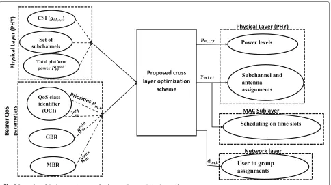
The channel state information from the physical layer would be the channel gain valuesgi,k,c,ton different
anten-nas and frequency-time slots for a userkwhich will be an
input to the cross-layer optimization procedure. The sets of subchannels assigned to the HAP and the total
avail-able powerPTotalPF of the platform are also passed by the
physical layer as an input to the cross-layer optimization procedure. The power allocation, subchannel allocation and antenna selection resulting from the solution scheme would be passed to the physical layer. The results of the chosen time slots will be passed to the scheduler in the MAC sublayer. The result of user to group admissions will
be passed to the network layer. Figure5illustrates input
parameters and outputs passed to the different layers for
the cross layer optimization problem (HAPEff).
5 Reducing the formulationHAPEffto a mixed binary polynomial constrained problem
In this section we show how the constraint setsC11 and
C12 in HAPEff are replaced by mixed binary
polyno-mial constraints (MBPCs), some of which are quadratic.
For constraint setC11 inHAPEff, the constraint can be
rewritten in the form:
log
Taking exponential of 2 for both sides of the constraint, we get:
Fig. 5Illustration of the inputs and outputs for the cross-layer optimization problem
which give the following set of equations:
wm,i,c,t=min
and the following inequality set becomes valid:
pm,i,c,t
Therefore constraint setC11 can be replaced by:
S
ForC12, the constraint set can be rewritten in the form:
log
taking the exponent of 2 for both sides we get:
S
which gives the following set of inequalities:
um,i,c,t=1+max
and the following inequality set becomes valid:
gi,k,c,tpm,i,c,tφm,k M
m=1 ∀i=igi,k,c,tpm,i,c,t+σ2
Therefore the constraintC12 can be replaced by:
given by (19) and (25) are second degree polynomial
(quadratic). Therefore replacing constraint sets C11 and
C12 in HAPEff with (18), (19), (24) and (25) gives a
mixed binary polynomial constraint program (MBPCP).
Section6shows how this is further reduced to a mixed
binary quadratically constrained program (MBQCP).
6 Reduction of the formulation to mixed binary quadratic constraints
Any MBPCP optimization problem maybe reduced to a MBQCP by the introduction of auxiliary variables and constraints to reduce all polynomial degrees to 2.
For example a cubic polynomial term x1x2x3 could be
modeled as x1X23 with X23 = x2x3. Using this
sim-ple reformulation technique, the polynomial constraints obtained in the previous section, can be converted to
mixed binary quadratic constraints by replacing (18) by
the following: ity constraints can be replaced by inequality constraints to give:
These sets replace the set ofM constraints in (18) with
3M + 2M.(S.C.T−3) quadratic constraints and adds
Again, this replaces the M constraints in (24) with
3M+2M.(S.C.T−3)quadratic constraints and addsM×
(S.C.T−2)new variablesUm,j.
The optimization problem is now an MBQCP given by:
Q1d:Wm,n−2≤wm,(n−1)wm,(n), ∀m
7 Comparison of the formulation sizes with the aid of a numerical example
In this section we illustrate the differences in the sizes of
the formulations (OP1) in [24] andHAPEffMBQCP. We
pro-vide P-Prob’s formulation (OP1) here for reference and comparison:
For the interpretation of the constraints we refer the reader to, [22–24]. Considering (OP1) in [24] first, we see that the number of variables are as follows:
• The number of binary variables,zm,i,k,c,t, is the productMSKCT
• The number of continuous variables,pm,i,c,t, isMSCT
• Hence, giving a total number of variables
VNOP1=MSKCT+MSCT. (32)
The number of constraints (excluding bounds and binary constraints) in each constraint set for (OP1) in [24] are as follows:
• Constraint setD1comprisesMSKCT constraints • Constraint setD2comprises
MSKCT[CT−1] [K−1]constraints
• Constraint setD3comprisesMSKCT constraints • Constraint setD4comprisesMSKCT constraints, • Constraint setD5comprises
MSKCT[M−1] [K−1]constraints
• Constraint setD6comprisesMSKCT constraints • Constraint setD7comprisesMSK constraints • Constraint setD9comprisesT constraints • Constraint setD10comprisesMSCT constraints
which all add up to
CNOP1=MSKCT[CT−1] [K−1] +MSKCT[M−1] [K−1] +4MSKCT+MSK+MSCT+T.
(33)
For the formulationHAPEffMBQCP, we have the following
numbers of variables:
• The numbers of binary variablesφm,k,θm,ym,i,c,tare
theMK, M and MSCT respectively giving a total number of binary variablesMK+M+MSCT. • The number of continuous variables:
– pm,i,c,tareMSCT,
– um,i,c,tareMSCT,
– wm,i,c,tareMSCT
– Um,jareM[SCT−2], and
all adding up to3MSCT+2M[SCT−2]continuous variables.
The number of binary and continuous variables add up to:
VN
HAPEffMBQCP =
4MSCT+2M[SCT−2]+MK+M.
(34)
The number of constraints (excluding bounds and
binary constraints) in each constraint set forHAPEffMBQCP
are as follows:
• Constraint setC1consists ofMK constraints • Constraint setC2consists ofSCT constraints • Constraint setC3consists ofMK constraints • Constraint setC4consists ofMSCT constraints • Constraint setC5consists ofMSCT constraints • Constraint setC6consists ofT constraints • Constraint setC8consists ofMSKCT constraints • Constraint setC9consists ofM constraints • Constraint setC10consists ofM constraints • Constraint setQ1aconsists ofM constraints • Constraint setQ1bconsists ofM[SCT−3]
constraints
• Constraint setQ1cconsists ofM[SCT−3]
constraints
• Constraint setQ1dconsists ofM constraints • Constraint setQ1econsists ofM constraints • Constraint setQ2consists ofMSKCT constraints • Constraint setQ3aconsists ofM constraints • Constraint setQ3bconsists ofM[SCT−3]
constraints
• Constraint setQ3cconsists ofM[SCT−3]
constraints
• Constraint setQ3dconsists ofM constraints • Constraint setQ3econsists ofM constraints • Constraint setQ4consists ofMSKCT constraints
which all add up to
CN
HAPEffMBQCP=
2MK+SCT+2MSCT+T+8M
+4M[SCT−3]+3MSKCT.
(35)
Finally, both the formulations (OP1) in [24] and
HAPEff
MBQCP consist of bilinear terms. By counting the
bilinear terms in (OP1) in [24] obtained from constraints
setsD3 andD4 we get:
NBiL HAPLagrange
2
=M2S2KCT+MSKCT. (36)
Also, by counting the bilinear terms in con-straint sets C8,Q1a,Q2,Q1b,Q1c,Q1d,Q1e,Q3a,
We graphically illustrate a comparison of efficiency
for the two formulations (OP1) in [24] andHAPEffMBQCP
in Figs. 6, 7, 8, 9 and 10. In these figures we
com-pare the number of binary variables, continuous vari-ables, total number of varivari-ables, number of constraints and number of bilinear terms for both formulations.
We refer to the indices m, i, k, c and t as the
prob-lem “dimensions". Therefore there are five dimensions for the problem in both formulations which are the num-ber of multicast sessions, the numnum-ber of HAP antennas on-board, the number of users in the service area, the number of sub-channels and the number of time slots respectively. We vary the dimensions of the problem as follows:
• The number of multicast sessionsM is varied in the range1−250.
• the number of antennas on-boardS is varied in the range1−20.
• the number of usersK in the service area is varied in the range1−500.
• the number of available sub-channelsC is varied in the range1−32.
• the number of available sub-channelsT is varied in the range1−24.
Figures 6, 7, 8, 9 and 10 are comprised of five plots
each in which one dimension is varied within its ranges mentioned above and the others are kept fixed at val-ues equal to their maximums in their respective ranges.
The results in Fig.6show that the number of binary
vari-ables forHAPEffMBQCP is way lower than those in (OP1)
in [24]. On the other hand in Fig.7, the number of
con-tinuous variablesHAPEffMBQCPare almost 4 times those of
(OP1) in [24] for the worst case. However by looking at
both Figs.6 and7, we can see that the number of
con-tinuous variables in both formulations are much lower than the binary variables which makes the total
num-ber of variables in Fig. 8 almost equivalent to the total
number of binary variables. Moreover, it is well known that when there are both binary variables and continu-ous variables in a problem, the binary variables are the main cause of algorithmic complexity involved in solv-ing the problem. Therefore, comparsolv-ing the numbers of continuous and binary variables in both formulations, we
see thatHAPEffMBQCPhas a much lower complexity
0 50 100 150 200 250 0
1 2 10
9
Old Formulation New Formulation
0 5 10 15 20
0 1 2 10
9
Old Formulation New Formulation
0 100 200 300 400 500
0 1 2 10
9
Old Formulation New Formulation
0 10 20 30
0 1 2 10
9
Old Formulation New Formulation
0 5 10 15 20 25
0 1 2 10
9
Old Formulation New Formulation
Number of Binary Variables
Fig. 6Illustration of the number of binary variables versus the different problem dimensions for (OP1) in [24] (old formulation) andHAPEffMBQCP (new formulation)
0 50 100 150 200 250
0 5 10 15 10
6
Old Formulation New Formulation
0 5 10 15 20
0 5 10 15 10
6
Old Formulation New Formulation
0 100 200 300 400 500
0 5 10 15 10
6
Old Formulation New Formulation
0 10 20 30
0 5 10 15 10
6
Old Formulation New Formulation
0 5 10 15 20 25
0 5 10 15 10
6
Old Formulation New Formulation
Number of Continuous Variables
Fig. 7Illustration of the number of continuous variables versus the different problem dimensions for (OP1) in [24] (old formulation) and HAPEff
0 50 100 150 200 250 0
1 2 10
9
Old Formulation New Formulation
0 5 10 15 20
0 1 2 10
9
Old Formulation New Formulation
0 100 200 300 400 500
0 1 2 10
9
Old Formulation New Formulation
0 10 20 30
0 1 2 10
9
Old Formulation New Formulation
0 5 10 15 20 25
0 1 2 10
9
Old Formulation New Formulation
Total Number Variables
Fig. 8Illustration of the total number of variables versus the different problem dimensions for (OP1) in [24] (old formulation) andHAPEff MBQCP(new
formulation)
0 50 100 150 200 250
0 5 10 10
14
Old Formulation New Formulation
0 5 10 15 20
0 5 10 10
14
Old Formulation New Formulation
0 100 200 300 400 500
0 5 10 10
14
Old Formulation New Formulation
0 10 20 30
0 5 10 10
14
Old Formulation New Formulation
0 5 10 15 20 25
0 5 10 10
14
Old Formulation New Formulation
Total Number of Constraints
Fig. 10Illustration of the total number of bilinear terms versus the different problem dimensions for (OP1) in [24] (old formulation) and HAPEff
MBQCP(new formulation)
Taking a look at the number of total constraints in
Fig. 9, we see that the number of constraints in
formu-lationHAPEffMBQCP is far lower than (OP1) in [24]. This
comes at the cost of up to three times larger number of
bilinear terms, in the worst case, for HAPEffMBQCP in all
dimensions as Fig. 10 shows. Notice the similar
behav-iors for both HAPEffMBQCP and (OP1) in [24] in Fig. 10
for each dimension. For the dimensions of the number of
multicast sessions, m, and the number of HAP antenna
onboard,i, the number of bilinear for both formulations
grow quadratically. For the other three dimensions, the growth is linear.
8 Proposed solution method: branching schemes and a presolving linearization-based
reformulation
This section explains how formulation HAPEffMBQCP is
solved. An approach similar to those in [32] and [27] is
used in which, an outer approximation is generated by linear underestimation of the non-convex quadratic con-straints to relax the problem’s feasible region. The
prob-lem becomes amixed binary linear program(MBLP) and
hence an LP solver can be used in a branch and cut
algo-rithm to solveHAPEffMBQCP.The branch-and-bound (BnB)
algorithm recursively splits the problem into smaller sub-problems, thereby creating a branching tree and implicitly
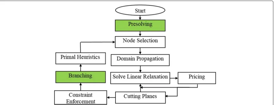
enumerating all potential solutions. At each subprob-lem, domain propagation is performed to exclude fur-ther values from the variables’ domains, and a relaxation may be solved to achieve an upper (dual) bound. The relaxation is then strengthened by adding further valid constraints, which cut off the optimum of the relax-ation. Primal heuristics are integrated in the BnB pro-cedure to improve the lower (primal) bound. The solver
used for the experiments is Solving Constraint Integer
Programs(SCIP) which is capable of solving a non-convex
mixed integer quadratically constraint program(MIQCP)
to optimality in finite time [33]. The interdependencies
between the algorithmic components of SCIP solver are
shown in Fig. 11. An explanation for the components
used in the experiments done for HAPEffMBQCP are
pro-vided in this section and Section8. The components are
the following:
• Presolving • Branching • Separating cuts • Domain propagation • Primal heuristics
The two components considered in this section are the
green colored boxes in Fig.11, which are presolving and
![Fig. 6 Illustration of the number of binary variables versus the different problem dimensions for (OP1) in [24] (old formulation) and HAPEffMBQCP(new formulation)](https://thumb-us.123doks.com/thumbv2/123dok_us/907841.1109647/18.595.58.539.415.706/illustration-variables-different-problem-dimensions-formulation-hapeffmbqcp-formulation.webp)
![Fig. 9 Illustration of the total number of constraints versus the different problem dimensions for (OP1) in [24] (old formulation) and HAPEffMBQCP(new formulation)](https://thumb-us.123doks.com/thumbv2/123dok_us/907841.1109647/19.595.59.540.84.358/illustration-constraints-different-problem-dimensions-formulation-hapeffmbqcp-formulation.webp)
![Fig. 10 Illustration of the total number of bilinear terms versus the different problem dimensions for (OP1) in [24] (old formulation) andHAPEffMBQCP (new formulation)](https://thumb-us.123doks.com/thumbv2/123dok_us/907841.1109647/20.595.53.542.79.353/illustration-bilinear-different-problem-dimensions-formulation-andhapeffmbqcp-formulation.webp)