T E C H N I C A L R E P O R T
Open Access
Evaluation of candidate geomagnetic field
models for IGRF-12
Erwan Thébault
1*, Christopher C. Finlay
2, Patrick Alken
3,4, Ciaran D. Beggan
5, Elisabeth Canet
6,
Arnaud Chulliat
3,4, Benoit Langlais
1, Vincent Lesur
7, Frank J. Lowes
8, Chandrasekharan Manoj
3,4,
Martin Rother
7and Reyko Schachtschneider
7Abstract
Background: The 12th revision of the International Geomagnetic Reference Field (IGRF) was issued in December 2014 by the International Association of Geomagnetism and Aeronomy (IAGA) Division V Working Group V-MOD (http://www.ngdc.noaa.gov/IAGA/vmod/igrf.html). This revision comprises new spherical harmonic main field models for epochs 2010.0 (DGRF-2010) and 2015.0 (IGRF-2015) and predictive linear secular variation for the interval
2015.0-2020.0 (SV-2010-2015).
Findings: The models were derived from weighted averages of candidate models submitted by ten international teams. Teams were led by the British Geological Survey (UK), DTU Space (Denmark), ISTerre (France), IZMIRAN (Russia), NOAA/NGDC (USA), GFZ Potsdam (Germany), NASA/GSFC (USA), IPGP (France), LPG Nantes (France), and ETH Zurich (Switzerland). Each candidate model was carefully evaluated and compared to all other models and a mean model using well-defined statistical criteria in the spectral domain and maps in the physical space. These analyses were made to pinpoint both troublesome coefficients and the geographical regions where the candidate models most significantly differ. Some models showed clear deviation from other candidate models. However, a majority of the task force members appointed by IAGA thought that the differences were not sufficient to exclude models that were well documented and based on different techniques.
Conclusions: The task force thus voted for and applied an iterative robust estimation scheme in space. In this paper, we report on the evaluations of the candidate models and provide details of the algorithm that was used to derive the IGRF-12 product.
Keywords: Geomagnetism; Field modeling; IGRF
Findings
Introduction
The International Association of Geomagnetism and Aeronomy (IAGA) released the 12th generation of the International Geomagnetic Reference Field (IGRF) in December 2014 (Thébault et al. 2015). The IGRF is a series of standard mathematical models describing the large-scale internal part of the Earth’s magnetic field between epochs 1900 A.D. and the present (see for instance Macmillan and Finlay 2011 for a review and Finlay et al. 2010a for the preceding generation). It is used by scientists
*Correspondence: [email protected]
1University of Nantes, Laboratoire de Planétologie et Géodynamique de Nantes, UMR 6112-CNRS, Nantes, France
Full list of author information is available at the end of the article
in a wide variety of studies including long-term dynam-ics of the Earth’s core field, space weather (e.g., Bilitza and Reinisch 2008), local magnetic anomalies imprinted in the Earth’s crust, or land surveying. It is also used by commercial organizations and individuals as a source of orientation information for drilling or navigation (Meyers and Minor Davis 1990) and has become of increasing interest for space science during the last decade. A task force appointed by IAGA approved the specifications of IGRF-12 and issued a call in May 2014. The call requested candidate models for the main field (MF) for the Definitive Geomagnetic Reference Field for epoch 2010 (DGRF-2010), for a provisional IGRF model for epoch 2015 (IGRF-2015) both to spherical harmonic (SH) degree 13, and for a prediction of its annual rate
of change, the secular variation (SV), over the upcoming 5 years (SV-2015-2020) to SH degree 8. The term “defini-tive” is used because any further substantial improvement of these retrospectively determined models is unlikely. In contrast, the provisional IGRF model will eventually be replaced by a definitive model in a future revision of the IGRF when the community will have more com-plete knowledge concerning the Earth’s magnetic field for epoch 2015.0.
Ten teams answered the call and submitted candi-date models. They were led by the British Geological Survey (UK), DTU Space (Denmark), ISTerre (France), IZMIRAN (Russia), NOAA/NGDC (USA), GFZ Potsdam (Germany), NASA/GSFC (USA), IPGP (France), LPG Nantes (France), and ETH Zurich (Switzerland). Seven candidate MF models for the DGRF epoch 2010.0, ten candidate MF models for the IGRF epoch 2015.0, and nine SV models for the predictive part covering epochs 2015.0-2020.0 were submitted for evaluation in October 2014 (see Table 1). The number of institutions participating in IGRF-12 was larger than for any previous generation. This reflects cooperation between scientists involved in modeling the magnetic field, the institutions archiving and disseminating the ground magnetic field data, and the national and the various space agencies who distribute well-documented magnetic satellite data from the satel-lite missions. Modellers made extensive use of the data from the international network of ground geomagnetic observatories either directly, or indirectly, in the form of magnetic indices monitoring the level of magnetic activi-ties. The candidate models were also primarily built using data from the German satellite CHAMP (2000-2010), the Danish satellite Ørsted (1999-), the Argentine-U.S.-Danish satellite SAC-C (2001-2013), and, especially for the epoch close to 2015.0, the European Swarm constellation (launched in November 2013; https://earth.esa.int/web/ guest/missions/esa-operational-eo-missions/swarm). The
teams adopted a variety of data selection, process-ing, and modeling procedures. Details concerning the techniques used to derive the individual candidate models can be found in the papers appearing in this special issue. Some teams derived their candi-date models from parent models describing the mag-netic field over periods longer than requested by IGRF (Finlay et al. 2015; Gillet et al. 2015; Hamilton et al. 2015; Sabaka et al. 2015). Such models involve inter-nal temporal parameterization using splines and exterinter-nal field parameterization of varying complexity and differ-ing reference frames. Such models co-estimate the vari-ous source fields through a grand inversion and perform a mathematical separation of the field into its inter-nal and exterinter-nal parts. Other teams focused their effort on dedicated internal candidate models for each of the epochs requested by the call, thus using data within win-dows centered on epochs of interest (Alken et al. 2015; Lesur et al. 2015; Saturnino et al. 2015; Vigneron et al. 2015). This necessarily involved less complex parameter-ization in space and in time and sometimes more drastic data selection and pre-processing to minimize the effects of unwanted magnetic field contributions arising from external fields. In general, all candidate models rely on some geographical and/or iterative statistical weighting schemes to down-weight measurements in particular geo-graphic regions or those poorly fit by the model. A special difficulty arises for the predictive SV part of the magnetic field for epochs 2015-2020. Forecasting the temporal evo-lution of the main geomagnetic field is no trivial matter. The geodynamo is a deterministic system with chaotic dynamics involving complex interaction of fluid flow and magnetic field within Earth’s core. A consistent prediction would therefore require a correct mathematical descrip-tion of these physical interacdescrip-tions which, despite impor-tant progress during the last decade, remains a frontier scientific subject. Some teams nevertheless considered a
Table 1Candidate models to IGRF-12 and participating organizations
Summary of submitted candidate models for IGRF-12
Team Model DGRF-2010 Model IGRF-2015 SV-2015-2020 Organization Publication
A YES YES YES BGS Hamilton et al. 2015
B YES YES YES DTU Space Finlay et al. 2015
C YES YES YES ISTerre Gillet at al. 2015
D YES YES YES IZMIRAN
-E YES YES YES NGDC-NOAA Alken et al. 2015
F YES YES YES GFZ Lesur et al. 2015
G YES NO YES NASA/GSCF
-H NO YES YES IPGP/CEA/LPG Nantes Fournier et al. 2015; Vigneron et al. 2015
I NO YES YES LPG Nantes Saturnino et al. 2015
-physics-based approach applying the tools of geophysi-cal assimilation (Fournier et al. 2015) or setting a pri-ori hypothesis on the core flow (e.g., Gillet et al. 2015; Hamilton et al. 2015). Other teams (e.g., Alken et al. 2015; Finlay et al. 2015; Lesur et al. 2015; Saturnino et al. 2015) relied on simple analytical extrapolation assuming that the magnetic field will evolve linearly over the next 5 years. From October to early December 2014, some members of the task force and interested parties carried out evaluations of the candidate models submitted by the different teams. In the call for IGRF-12, the internal field (“main field”) was requested to degree and order 13 for epochs 2010.0 and 2015.0. Some teams interpreted this as requesting all global scale fields whose sources were internal, while other teams interpreted it as referring only to contributions from the Earth’s “core” field. The notion, of course, could be clarified by IAGA but this ambiguity helps to ensures that some candidate models are indepen-dent and aids in making the standard model valid on aver-age for a wide range of disparate scientific applications. Such variety amongst the candidate models, however, often complicated the work of the evaluators. Assessment of candidate models was primarily based on statistical criteria. Some MF and SV models showed greater con-sistency than others. However, good statistical agreement between models does not necessarily mean that these models are the most realistic. It can also be a consequence of them using very similar data selection or modeling techniques. For this reason, the evaluators also relied on the companion descriptions of the candidate model sub-mitted for evaluation and finally often on their empirical experience.
The first section of this paper summarizes the statistical criteria used by the task force members and the evaluators for the testing and the inter-comparison of the candidate models to IGRF-12. The results of this analysis that served as the basis for internal discussion are then detailed. The task force chair prepared a ballot paper containing a selec-tion of weighting opselec-tions that was voted on by the task force in December 2014. The last section gives some details of adopted weighting scheme. The resulting IGRF-12 coefficients were prepared and checked before being made available to the public through the IAGA Div V, WG V-MOD webpage http://www.ngdc.noaa.gov/IAGA/ vmod/igrf.html before 1 January 2015.
Mathematical definitions and criteria used in evaluations We present the formulae employed by the task force mem-bers and the evaluators using the notation of Finlay et al. (2010b). The IGRF is a series of mathematical models of the internal geomagnetic fieldB(r,θ,φ,t)and its annual rate of change (secular variation - SV). On and above the Earth’s surface, assumingμ = μ0 and no local electric current, the magnetic field B is defined in terms of a
magnetic scalar potential V by B = −∇V and where in spherical polar coordinatesV is approximated by the finite series
with r denoting the radial distance from the center of the Earth,a = 6371.2 km being the Earth’s mean ref-erence spherical radius conventionally used in geomag-netic modelling,θ denoting geocentric co-latitude, andφ denoting east longitude. The functionsPmn(cosθ)are the Schmidt quasi-normalized associated Legendre functions of degreenand orderm. The Gauss coefficientsgmn,hmn are functions of timetand are conventionally given in units of nano-Tesla (nT).
• Difference between models
Evaluations often involve differences between a candi-date modeliwhose coefficients are denoted byignm and ihmn and another model whose coefficients are labelledj and denoted byjgnmandjhmn. The differences between the coefficients of two such models denoted by
i,jgnm=ignm−jgnm and i,jhmn =ihmn −jhmn, (2)
are sometimes analyzed coefficient by coefficient. Due to linearity, they may also be used to compute the difference between the models’ magnetic field components using the gradient of Eq. 1 in the spatial domain on a reference sphere, such as the Earth’s mean radiusr= aor the core mantle boundary atr=3485 km.
• Weighted mean model
Comparisons between candidate models are also often made with respect to their differences from the mean model estimated from theKcandidate models. The sim-ple arithmetic mean model is defined by the coefficients
gm
This special case corresponding to all candidate mod-els having identical unit weight can be generalized. Each modelican be allocated a certain weightiwmn that varies with the degreenand orderm. The Gauss coefficients of such a weighted mean model are then
In previous generations of IGRF, the evaluation process led to some estimates of the individual weights iwmn in order to calculate weighted mean (Finlay et al. 2010b, for instance). We will discuss below some of the arithmetic weighted means suggested by some evaluators in the case of IGRF-12. In the following, we also compute the median model from the K candidate models that is expected to be less influenced by a small number of models showing strong discrepancies.
• Spherical harmonic power spectrum and total root
mean square vector field
The mean square vector field averaged over the spher-ical surface of a candidate model expanded in spherspher-ical harmonics (Eq. 1) per spherical harmonic degreei,0Rnis defined by (see for example, Lowes 1966; 1974)
i,0Rn=(n+1)
This so-called Lowes-Mauersberger geomagnetic power spectrum is also computed for the difference between two modelsiandjand denotedi,jRnsuch that trum of Eq. 5 can be calculated on any spherical surface of radiusrwhere the magnetic field is source free. Com-parisons are then often carried out at the Earth’s mean spherical surface r = a, which corresponds to the sur-face where the IGRF standard model is often employed by users. Summing the power spectrumi,jRn(Eq. 6) over degreesnfrom 1 to the truncation degreeNof the model provides the mean square vector field at the altitude r. Then, taking the square root yields the root mean square (RMS) vector difference field between the modelsiandj
i,jR=
In addition to calculating the RMS difference between two modelsiandj, we can define and compute the mean value of the RMS difference of theith model to the(K−1)
In the following, we also estimate the RMS error due to the rounding of the candidate models. For a given pre-cisionp, each Gauss coefficient has a standard deviation due to the rounding error equal top/√12 (see also Lowes 2000). The RMSRpof the truncation error then equals
Rp=p/
When analyzing the difference between two individual candidate models, it is sometimes informative to com-pute the azimuthal rather than the Lowes-Mauersberger geomagnetic power spectrum of their difference. For this, we re-organize the square of the coefficients as a func-tion of the azimuthal ratio az = m/n, which varies from 0 for purely zonal terms to 1 for sectoral terms (see Sabaka et al. 2004 for a description of the procedure) and we define az positive for the i,jgnm and negative for the i,jhmn model coefficients. This azimuthal power spectrum is denotedi,jRa.
• Sensitivity matrix
One can also analyze the difference between two models (Eq. 2) normalized by the Lowes-Mauersberger geomag-netic power spectrum. This so-called sensitivity matrix S(n,m)expressed in percent for each degreenand order
Finally, two models may have systematic differences in amplitude causing large RMS but still be linearly corre-lated. The correlation per degree between two modelsi,jρn is the quantity (Langel and Hinze 1998, p. 81)
i,jρn=
which is, following the standard definition of the Pearson’s correlation coefficient, the covariance between two mod-els divided by the product of their standard deviation. It gives 1 for a full positive correlation, 0 for no correlation, and−1 for a full anticorrelation degree per degree.
Evaluation of main field candidate models Analysis of DGRF-2010 candidate models
Table 2 lists the seven candidate models received for evaluation for epoch 2010.0. The teams are identified with capital letters and major information about the data sources used and very brief comments concerning the various modeling approaches adopted are included. The teams derived their candidate from parent models (see Table 1 for the list of references) and evaluated these parent models at epoch 2010.0.
In Table 3, we present the RMS vector field differences i,jR(Eq. 7 in nT) between the individual candidate mod-elsiandjat the Earth’s reference radiusr = a. The two last columns show the RMS difference between each can-didate modeliand the simple arithmetic mean modelM (Eq. 3) and to the median modelMmed. The requested pre-cision ofp = 0.01 nT leads to an estimate of the error due to truncation (Eq. 9) equal toRp=0.13 nT. All mod-els show RMS differences well above this value showing the effect of the varying modeling strategies adopted by the different teams. Models A, B, E, and F are in closer agreement with the arithmetic mean and median models than models C, D, and G. The RMS difference between each model of this first group is also smaller than the RMS difference between models of the second. The final row of Table 3 gives the arithmetic means of the RMS vector field differences ofi,jRof modelifrom the other models jconfirm that A, B, E, and F have the smallestiR. Model C is the most discrepant model with a mean RMS differ-ence to all models almost 1.8 larger than the model A to all models.
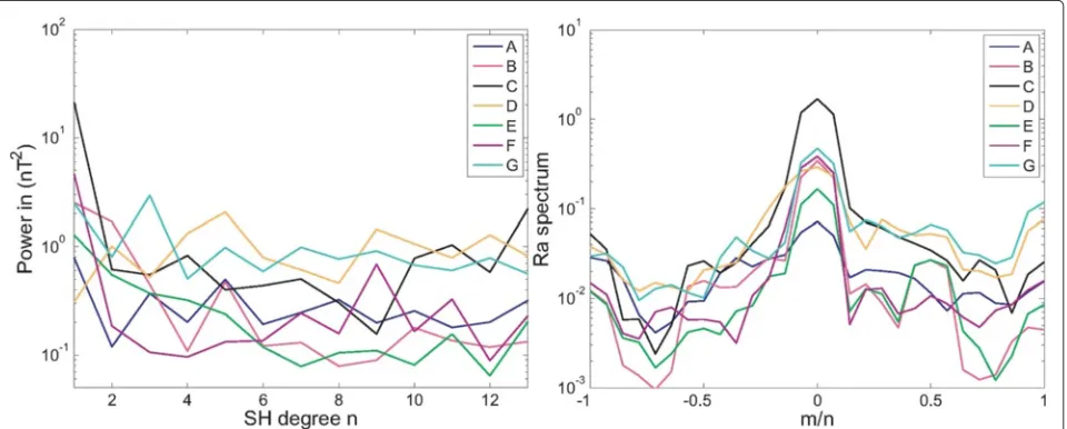
These general features are confirmed by Fig. 1-left which presents the Lowes-Mauersberger spectra i,MRn (defined in Eq. 6) of the difference between DGRF-2010 candidate models and the simple arithmetic mean model
M. The three models C, D, and G are noticeably differ-ent from the mean. Differences between the models are largest for the dipole term. The maximum deviation is found for the dipole term for model C, and large differ-ences are visible forn = 5 for model D and forn = 3 for model G. The azimuthal power spectra i,jRa of the difference between all candidate models and the mean model shown in Fig. 1-right provide additional informa-tion. All models differ for the axial dipole term (az= 0), and their spectra show two wings for az ±1. The increasing difference between all models for the sectoral coefficients illustrates a problem inherent to the available satellite magnetic field measurements. Because of rapid external field variations, the vector satellite data have cor-related errors along the near polar circular satellite orbits that do not allow accurate recovery of the magnetic field components perpendicular to the flight direction. In addi-tion, models using mostly scalar measurements in some geographical regions, for instance over the Earth’s polar caps, may also be subject to the “Backus effect” (Backus 1970) that causes an ambiguity also on the sectoral Gauss coefficients. We are dealing here with features that are well known to modellers and evaluators and for which an objective evaluation is challenging. However, notice-able differences occur for models C, D, and G at positive azimuthal numbers (corresponding to ignm coefficients) whose origin is not easy to determine.
Further information is provided by the analysis of the coefficient by coefficient difference i,jgnm as defined in Eq. 2 between each candidate model and the simple arith-metic mean model (a comparison with the median showed similar general features). The comparison is made here using a logarithmic scale to better highlight the differences
Table 2Summary of DGRF-2010 candidate models submitted to IGRF-12
DGRF candidate models for main field epoch 2010
Team Model Organization Data Comments (parent model etc.)
A DGRF-2010-A BGS Ørsted; CHAMP; Swarm A, B, C; Based on parent model using order 6 B-splines Observatory hourly means with 1 year knot spacing
B DGRF-2010-B DTU Space Ørsted; CHAMP; SAC-C; Swarm A, B, C; Based on CHAOS-5
Observatory monthly means using order 6 splines with 6 months spacing
C DGRF-2010 ISTerre Ørsted; SAC-C; CHAMP; Swarm B Based on COV-OBS.x1
observatory monthly mean using order 4 B-splines with 2 year spacing
D DGRF-2010-D IZMIRAN CHAMP 2009.0-2010.75 Spherical Harmonics for each day
no data selection but numerical filtering then linear regression centered on 2010.0
E DGRF-2010-E NGDC-NOAA CHAMP Based on parent model using quadratic expansion
F DGRF-2010-F GFZ CHAMP from 2009.0 to 2011.0 Based on parent model using order 6 B-splines
USTHB/EOST observatory hourly means with 6 month spacing
G DGRF-2010-G NASA/GSFC Ørsted; CHAMP; SAC-C Based on CM5
Table 3RMS vector field differencesi,jRin units nT between DGRF-2010 candidate models and also between candidates and the
arithmetic mean reference modelsMand median reference modelMmedin the rightmost columns. The bottom two rows are simple arithmetic meansiRof thei,jRwhere the means include all candidates
i,jR/ nT A B C D E F G M Mmed
A 0.00 2.76 6.61 4.01 2.40 2.55 4.92 1.97 1.70
B 2.76 0.00 7.06 4.91 2.04 2.37 5.38 2.50 1.96
C 6.61 7.06 0.00 7.28 6.72 7.66 5.81 5.45 5.99
D 4.01 4.91 7.28 0.00 4.27 4.52 5.66 3.53 3.72
E 2.40 2.04 6.72 4.27 0.00 2.42 4.81 1.92 1.51
F 2.55 2.37 7.66 4.52 2.42 0.00 5.47 2.68 2.18
G 4.92 5.38 5.81 5.66 4.81 5.47 0.00 3.69 4.19
Mean Diff 3.88 4.09 6.86 5.11 3.78 4.17 5.34 3.10 3.04
at low SH degrees. Figure 2-left illustrates that differences for all models are indeed comparatively larger for the zonal terms (m = 0) and more particularly for the axial dipole coefficientg01. This well-known feature is related to the difficulty in accurately separating the large-scale main internal and external magnetospheric fields given the available data (e.g., Olsen et al. 2010, Thébault et al. 2012). Interestingly, although models A, B, E, and F have small RMS differences to the mean, they differ more in their dipole coefficients than at other degrees. Model C has the strongest deviation for itsg10 term compared to other candidate models but otherwise compares reason-ably well with the mean model from SH degrees larger than 2. This informs us that the comparatively large RMS displayed in Table 3 for this model is mostly due to a dif-ference on the axial dipole coefficient. Candidate models D and G further show clear deviations at larger SH degrees such as for SH degreen= 5 and orderm= 0 for model
D andn=3 and orderm=0 for model G. The spherical degree correlationi,Mρnas defined in Eq. 11 between the DGRF-2010 candidate models and the arithmetic mean modelMis shown in Fig. 2-right. All models correlate well up to SH degree 10. Again, the degree correlation of can-didates C, D, and G toMabove SH degree 10 is slightly lower than that of A, B, E, and F which appear close to M. The most noticeable differences occur for candidate C at degree 13 but with a correlation better than 0.99 illus-trating the high level of correlation between all candidate models despite these statistical differences.
A final analysis is provided by the differences between the candidate models and the simple arithmetic mean model Min space. In Fig. 3, we show the radial compo-nent of these differences calculated at the Earth’s refer-ence mean radiusr = a. Visual inspection reveals some additional disparities between the candidate models. The residual fields for candidate models A, B, E, and F show
Fig. 1Left plotshows the Lowes-Mauersberger spectrai,MRnfrom Eq. 5 of the difference between the DGRF-2010 candidate models and the simple
Fig. 2Left plotshows differencesi,jgmn as defined in Eq. 2 between DGRF-2010 candidate models and their arithmetic mean modelMas a function of
the index of the spherical harmonic coefficient (running fromg0
1,g11,h11,g02,h11, etc. indexed 1,2,3,4,5, etc). The vertical line locates the zonal coefficient (m=0) for each SH degreen.Right plotshows the SH degree correlationi,Mρn(Eq. 11) of DGRF-2010 candidate models with the
arithmetic mean modelM
clear but weak dipolar signatures. The residuals for model A, B, E, and F are mostly positive in the northern hemi-sphere and negative in the southern hemihemi-sphere. The sign in the polar regions is different between the group of can-didate models comprising C, D, and G and the group of candidate models comprising A, B, E, and F. The candi-date model C involves the most striking deviations from M, locally as large as 20 nT. This large difference implies that the simple arithmetic mean model is probably biased towards model C for the dipole terms. This also illustrates one of the limitations of testing the candidate models against the simple arithmetic mean modelM. Apart from these general large-scale dipolar structures, the residual maps show that the differences are not confined to any particular geographical location except for models D and G. For model D, we see a positive signature following the magnetic equator. We recall that model D is the only model that does not rely on data selection in time while other candidate models select measurements according to the local time to mitigate the leakage of the diurnal iono-spheric magnetic field. Therefore, candidate model D may be contaminated by small scales with structures character-istic of the equatorial electrojet (EEJ) ionospheric field at noon local time. Model G has a large-scale structure that arises from the difference at SH degree 3 and order 0. Can-didate model G is the only model among the canCan-didates that seeks to estimate and then to explicitly remove the ionospheric night-time primary and induced contribution (Sabaka et al. 2015) that mostly contribute to zonal terms of SH degree 1 and 3. Nearly two-thirds of the variance between models G andMcan be explained by the removal or inclusion of the night-time ionospheric induced field,
respectively. Models D and G therefore rely on two differ-ent interpretations of how to best construct the IGRF for its disparate community of users.
Analysis of IGRF candidate models for epoch 2015
Fig. 3Difference in nT in the radialBrcomponent of the magnetic field between each DGRF-2010 candidate model (labeled with capital letter, see
Table 4Summary of IGRF-2015 candidate models submitted to IGRF-12
IGRF candidate models for main field epoch 2015
Team Model Organization Data Comments (parent model, propagation to 2015)
A IGRF-2015-A BGS Ørsted; CHAMP; Swarm A, B, C; Based on parent model evaluated in 2015.0 Observatory hourly means extrapolation from steady core flow hypothesis
B IGRF-2015-B DTU Space Ørsted; CHAMP; SAC-C; Swarm A, B, C; Parent CHAOS-5 evaluated in 2015.0 Observatory monthly means linear extrapolation from 2014.75
C IGRF-2015-C ISTerre Ørsted; SAC-C; CHAMP; Swarm B Parent COV-OBS.x1 model evaluated in 2015 observatory monthly mean using forward integration of a stochastic model
D IGRF-2015-D IZMIRAN Swarm A, B, and C vector data Parent model evaluated in 2015.0 Nov-2013 to Sep-2014, no data selection linear extrapolation
E IGRF-2015-E NGDC-NOAA Ørsted; Swarm A, B, C Parent model evaluated in 2015.0
linear extrapolation from 2014.3
F IGRF-2015-F GFZ Swarm A, B, C; Parent model evaluated in 2015.0
USTHB/EOST observatory hourly means lineral extrapolation from 2014.5
H IGRF-2015-H IPGP Swarm A, B, C Nov-2013 to Sep-2014 Parent model evaluated in 2015.0 CEA/CNES only ASM experimental vector data
I IGRF-2015-I LPG Nantes Swarm A and C Parent model evaluated in 2015.0
CNES Nov-2013 to Sep-2014 linear extrapolation from 2014.3
J IGRF-2015-J ETH Zurich Swarm C; Parent model evaluated in 2015.0
GFZ Dec-2013 to Sep-2014 linear extrapolation
less than 10 nT but models D and J show significantly larger deviations. Compared with the RMS to the mean model, the RMS to the median model are reduced for can-didates A, B, E, F, and H suggesting a better agreement between these five models than between C, D, I, and J.
Figure 4-left indeed confirms that models D and J show noticeable differences over all SH degrees and are statis-tically significantly different from the mean model. The model I compares better to the mean model for the SH degree 1–3 but the differences then increase with the
degree and finally differs from theMmodel as much as models D and J at larger SH degrees. Model C shows a significant deviation for SH degrees 1–3 but then a bet-ter agreement to the mean model at larger SH degrees. A, B, E, F, and H models have comparable mean square dif-ference to the mean model at all SH degrees except for H which deviates significantly for SH degrees 4–6. Models D, I, and J exhibit a saw-tooth behavior that could indi-cate the presence of aliasing or at least illustrate difficulties with noise being mapped into some model coefficients at
Table 5RMS vector field differencesi,jRin units of nT between IGRF-2015 candidates and also between them and the arithmetic mean
of all candidatesMand the medianMmed. The bottom row displays the mean of the RMS vector field differences between each candidate model and all other candidate modelsiRfrom Eq. 8 labelled “Mean Diff”
i,jR/ nT A B C D E F H I J M Mmed
A 0.0 6.8 12.1 14.1 7.3 6.3 9.1 10.3 16.2 6.2 5.8
B 6.8 0.0 9.8 13.3 4.8 5.1 5.4 9.3 15.3 3.8 3.2
C 12.1 9.8 0.0 17.0 12.5 10.1 10.9 11.8 15.4 8.8 8.9
D 14.1 13.3 17.0 0.0 14.3 12.9 16.1 14.5 18.4 11.8 12.6
E 7.3 4.8 12.5 14.3 0.0 6.5 7.0 9.9 16.3 5.8 5.2
F 6.3 5.1 10.1 12.9 6.5 0.0 7.6 9.2 15.0 4.1 3.5
H 9.1 5.4 10.9 16.1 7.0 7.6 0.0 11.8 17.3 7.0 6.4
I 10.3 9.3 11.8 14.5 9.9 9.2 11.8 0.0 14.9 7.4 7.8
J 16.2 15.3 15.4 18.4 16.3 15.0 17.3 14.9 0.0 12.9 13.8
Fig. 4Lowes-Mauersberger spectrai,MRnfrom Eq. 5 of the difference between the IGRF-2015 candidate models and the simple arithmetic mean
modelMat the Earth’s mean radiusr=a. Theright plotshows the azimuthal power spectrumi,MRaof this difference
all SH degrees. The azimuthal power spectrum (Fig. 4-right) shows general differences that are larger in the zonal and the sectoral harmonics for all candidate models with some exceptions for models D and J. The differences for candidate models A, B, and F are clearly lower than for other candidate models at low SH orders. Candidate model A has, however, comparatively larger differences for the sectoral than for the zonal terms. On the contrary, the model H is in better agreement with the mean model at larger SH orders but agrees less well at low SH orders.
The absolute coefficient by coefficient differences between the candidates and the mean model (Fig. 5-left)
shows that candidate model C is the most different for the axial dipole term. The largest difference in magnitude is for the coefficienth11 of the candidate model J. Model H is close to the mean model for the zonal terms for SH degrees 2 and 3 but then increases for zonal terms for SH degrees 4–6, which explains the rise in the power spectrum of its difference to the mean model for these degrees (Fig. 4-left). All candidate models have differences decreasing in magnitude with the SH degree with the exception of model D which shows largest differences at all SH degrees and low orders. Figure 5-right indeed illus-trates that model D has the smallest correlation to the
Fig. 5Left plotshows differencesi,jgmn as defined in Eq. 2 between IGRF-2015 candidate models and their arithmetic mean modelMas a function of
the index of the spherical harmonic coefficient (running fromg01,g11,h11,g02,h11etc indexed 1,2,3,4,5, etc). Thevertical linelocates the zonal coefficient (m=0) for each SH degreen.Right plotshows the SH degree correlationi,Mρn(Eq. 11) of IGRF-2015 candidate models with the arithmetic mean
mean model at large degreesnwith a most significant dif-ference from SH degree 11, thus corresponding to small spatial scales. Models B, E, and F show the best correlation through all SH degrees.
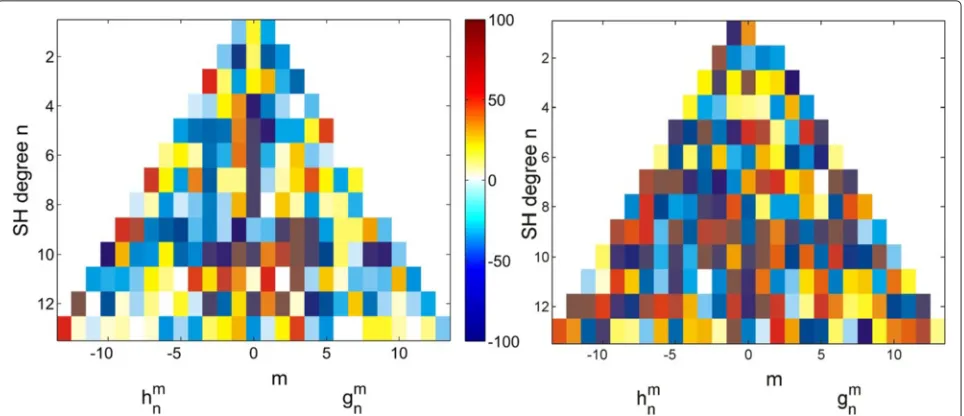
The Fig. 6 compares the sensitivity matrix S(n,m) as defined by Eq. 10 of the difference between candidate model B and the mean modelM(left) and also between the candidate model J and the mean modelM(right). It shows that the mismatch between the coefficients of the candidate model B and theMis about 18 %. For model J, the mismatch is twice as large and about 40 % on aver-age. All other candidate models show differences for each coefficients between these two extreme cases.
In the residual maps shown in Fig. 7 at the Earth’s refer-ence surface, we see that models B and F have the smallest deviation to the mean model with no specific spatial struc-tures. Models E and I show large-scale residuals as antici-pated by the Fig. 5-left indicating that most differences to the mean model are for coefficients of low SH degree. All other residual maps have different characteristics. Model A possesses low latitude anomalies linked to its anoma-lous sectoral harmonics (Fig. 4-right). For models C, E, and H, large-scale residual structures are noticeable with model C showing again a strong global opposite sign com-pared to other models. Models D, H, I, and J show also strong differences in the polar areas and to a lesser extent along the dip equator. Since these models were built upon Swarm measurements over less than a year, some of the polar regions may not yet have been sufficiently surveyed to separate the internal and external fields (especially for those models relying on night time data selections). The residual structures for candidate model D are prominent
at low latitudes and a contamination of external iono-spheric field is likely. Model J is strikingly different from all other candidate models. The residual map is peculiar and not easily explained from the description of the model parameterization or the data selection.
Analysis of IGRF-12 SV-2010-2015 candidate models
The final evaluation was for candidates submitted for the IGRF-12 average predictive SV for the interval 2015-2020. In this section, the Gauss coefficientsgnmandhmn refer to the predicted annual average rate of change in the coef-ficients between epochs 2015.0 and 2020.0 and are now given in units of nT/yr. The call requested candidate mod-els to 0.1 nT/yr precision and up to SH degree 8. Nine teams submitted SV-2015-2020 candidate models. Seven of these teams also submitted candidate models to DGRF-2010 or to IGRF-2015 (A, B, C, D, E, F, and I). Candidate models G and H were submitted by the same lead insti-tutions (respectively NASA and IPGP) but prepared by independent teams in collaboration with different part-ners. The colors used for these two candidate models in the following line plots are thus different from the ones used in previous sections in order to avoid confusion. Important details about the team models submitted for SV are collected for reference in Table 6. Five of these models rely on mathematical extrapolation of parent models (B, D, E, F, and I). Two of them (models G and H) rely on geody-namo simulation based on a model of core dynamics and assimilation of magnetic field models in SH in order to obtain a SV forecast for the upcoming 5 years. The last two candidate models rely on statistical analyses of the main magnetic field variation over the past centuries and on
Fig. 7Difference in nT in the radialBrcomponent of the magnetic field between each IGRF-2015 candidate model (labeled with capital letter, see
Table 6Summary of SV-2015-2020 candidate models submitted to IGRF-12
Predictive SV candidate models for epoch 2015-2020
Team Model Organization Data Comments (parent model, propagation to 2015)
A SV-2015-2020-A BGS Ørsted; CHAMP; Swarm A, B, C; Based on core flow parent model evaluated Observatory hourly means and averaged SV from 2015.0 to 2020.0
B SV-2015-2020-B DTU Space Ørsted; CHAMP; SAC-C; Swarm A, B, C; Based on parent CHAOS-5 model Observatory monthly means evaluated from splines at 2014.0
C SV-2015-2020-C ISTerre Ørsted; SAC-C; CHAMP; Swarm B Based on parent ensemble COV-OBS.x1 model observatory monthly mean evaluated and averaged SV from 2015.0 to 2020.0
D SV-2015-2020-D IZMIRAN Swarm A, B, C Natural orthogonal components (NOCs)
Nov-2013 to Sep-2014, no data selection estimated at 2014.7 (sept-2014)
E SV-2015-2020-E NGDC-NOAA Ørsted; Swarm A, B, C From parent model
first-order Taylor series with slope at 2015.0
F SV-2015-2020-F GFZ Swarm A, B, C; From parent model
USTHB/EOST observatory hourly means evaluated and averaged SV from 2013.5 to 2014.5
G SV-2015-2020-G NASA Geodynamo simulation and assimilation from CALS3K.2,
UMBC gufm1, CM4, CHAOS-4+; average SV from 2015.0 to 2020.0
H SV-2015-2020-H IPGP Swarm A, B, C Geodynamo simulation and assimilation from Swarm
LPG Nantes evaluated and averaged SV from 2015.0 to 2020.0
I SV-2015-2020-I LPG Nantes Swarm A and C From parent model
CNES Nov-2013 to Sep-2014 first-order Taylor series with slope at 2014.3
core flow hypotheses to forecast the field (candidate mod-els A and C). This is the first time that the call for IGRF candidate models received so many contributions relying on physical assumptions concerning the flow in the Earth’s core.
The simple mathematical extrapolations are often poor predictors as was illustrated by Finlay et al. (2010b, their figure thirteen). For this reason, models B, D, E, F, and I propose candidate models to the SV centered on an epoch close to the available data that does not exceed 2015.0. Forecasting the field to more distant epochs is numeri-cally easier with physinumeri-cally based models although they
also have a limited horizon of predictability (for instance Lhuillier et al. 2011). The teams who favored the physically based approach therefore submitted candidates averaged over the upcoming 5 years and centered them on epoch 2017.5. These two families of candidate models, here-after referred to as the mathematical and physical models therefore follow distinct philosophies. The mathematical models aim to better predict the main field changes for the next 1–2 years simply assuming that its rate of change will be statistically identical to the one observed in recent epochs. On the contrary, physical models hope to predict the field better on average over the full 5-year interval.
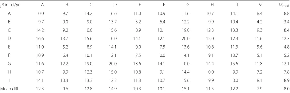
Table 7RMS vector field differencesi,jRin units nT/yr between SV-2015-2020 candidate models and also between these and the mean
modelMand the median modelMmed. The final row labelled “Mean Diff” is the meaniRof thei,jRfor each candidate or mean model
i,jRin nT/yr A B C D E F G H I M Mmed
A 0.0 9.7 14.2 16.6 11.0 10.9 11.6 10.7 14.1 8.4 8.8
B 9.7 0.0 9.0 13.7 5.2 6.4 12.2 9.9 10.4 4.2 3.4
C 14.2 9.0 0.0 15.6 8.9 10.1 19.0 12.3 13.3 9.3 8.4
D 16.6 13.7 15.6 0.0 14.1 12.1 20.0 15.0 12.3 11.6 12.3
E 11.0 5.2 8.9 14.1 0.0 7.5 13.6 10.8 11.3 5.6 4.8
F 10.9 6.4 10.1 12.1 7.5 0.0 14.1 9.1 10.7 5.1 5.2
G 11.6 12.2 19.0 20.0 13.6 14.1 0.0 14.4 15.6 11.8 12.1
H 10.7 9.9 12.3 15.0 10.8 9.1 14.4 0.0 9.9 7.2 7.8
I 14.1 10.4 13.3 12.3 11.3 10.7 15.6 9.9 0.0 8.1 8.9
Table 7 shows that there is a much wider scatter of differences between the candidate models for SV-2015.0-2020 than between those for the main field at epochs 2010.0 and 2015.0. This reflects the difference between the two strategies adopted by the teams and the intrin-sic difficulty in forecasting the change of the magnetic field. The mean RMS of the difference between the can-didate and the simple arithmetic mean models is between 4.2 nT/yr for model B and 11.8 nT/yr for model G at the Earth’s reference radiusr = a. Mathematical models B, E, and F show less scatter about the mean and median models but there is no systematically better agreement with the other mathematical models. Models A and H, for instance, have lower RMS to the mean than models D and I, both belonging to the family of mathematical models (note that model D is not extrapolated but estimated in 2014.7; i.e, in September 2014). Therefore, mathematical and physically based models do not show complete inter-nal consistency within their group, although the physical models in general show larger RMS between themselves than the mathematical models.
The power spectrum of the difference to the simple arithmetic mean model M (Fig. 8-left) shows that the largest difference for models (C, D, and G) are for the SH degrees 1–3. In particular, the model G is the most notably different model. Models B, E, and F have similar differ-ences over all SH degrees. The difference to the mean model for other models do not have clear characteris-tics except maybe for model A, showing a large difference for SH degree 5, and for model I, comparing well to the mean model up to SH degree 4 but then showing stronger differences. Figure 8-right shows that the coef-ficients hm
n of models C and G are particularly different from the mean model coefficients. The candidate model A
shows differences that distribute over all SH degrees and orders. For the other models, we recognize the now famil-iar central and side increased differences in the azimuthal spectrum corresponding to difficulties in recovering the zonal and the sectoral terms, because of internal/external field separation and noise correlated along the satellite orbits.
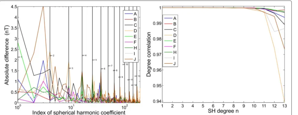
Table 7 suggests that models D and G show the largest differences. This is confirmed by Fig. 9-left showing the absolute value of the difference to the mean model coef-ficient by coefcoef-ficient. The largest absolute differences of more than 5 and 3.5 nT/yr are seen on the coefficients h11andh12of model G. Note that model C also has strong anomalous values for these coefficients. Model D is dis-similar for the zonal term as anticipated by Fig. 8-right, in particular on coefficientg02. In spite of these differences, we learn from Fig. 9-right that candidate model A is the least correlated on average to the mean model with in par-ticular a significant loss of correlation to the mean model M from SH degree 4. There appears to be no obvious way to choose between the candidates and to ascertain which are valid as the conclusions differ depending on the selected criterion. Therefore, it is instructive to look at the difference maps (Fig. 10). They confirm that few mod-els are similar to each other. The best agreement is for models B, E, and F. This is to be expected because these three candidates rely on similar mathematical modeling procedures. Some mathematical models relying on Swarm magnetic field measurements only (D and I) show increas-ing differences in the polar regions possibly comincreas-ing from the fact that the time window covered by the available data is too small to constrain accurately the SV up to SH degree 8. Models C and G exhibit two strong patches of opposite sign whose origin is unclear. For physically
Fig. 8Lowes-Mauersberger spectrai,MRnfrom Eq. 5 of the difference between the SV-2015-2020 candidate models and the simple arithmetic mean
Fig. 9Left plotshows differencesi,jgmn as defined in Eq. 2 between SV-2015-2020 candidate models and their arithmetic mean modelMas a function
of the index of the spherical harmonic coefficient (running fromg0
1,g11,h11,g02,h11etc indexed 1,2,3,4,5, etc). Thevertical linelocates the zonal coefficient (m=0) for each SH degreen.Right plotshows the SH degree correlationi,Mρn(Eq. 11) of SV-2015-2020 candidate models with the
arithmetic mean modelM
based models (A, C, G, and H), we expect some differ-ences at small spatial scales as each of them is given as an average over the 5-year interval. This construction tends to generate candidate models with smoother small scales compared to mathematical models providing candidates as snapshots at a given epoch. Interestingly, the residual map for the SV candidate model A when compared to the mean model is similar in shape to the residual map that was observed between the IGRF-2015 candidate model A and the mean model (Fig. 7). This suggests that most of the observed difference to the arithmetic mean model for epoch 2015.0 was caused by the SV model used to forecast the main field from earlier epoch to epoch 2015.0. Simi-lar correlations between the differences of IGRF-2015 and SV-2015-2020 candidate models to the arithmetic mean models are found for candidate models C, E, and I. As was the case for DGRF-2010 and IGRF-2015, there are clearly features in some models which are not in consensus with others, though it is impossible to ascertain which are valid.
Weighting scheme applied to derive the IGRF-12 models The analyses described above were used by the task force members in order to inform the construction of the IGRF-12 models out of theKcandidate modelsix=
igmn,ihmn
submitted by the different teams for DGRF-2010, IGRF-2015, and SV-2015-2020. The mathematical problem is the following. We wish to average over the ix so as to obtain the most accurate estimate of x0, the “true” field. Assuming that theixcontains only random errors and given no other information about their relative ran-dom errors, the standard least squares (LS) is the best linear estimator. It assumes that each of the K models
are samples from the same probability density function. Minimizing the functional arithmetic mean in which eachixis given equal weight. The varianceσ2, the mean-square error of theix about x0, can then be estimated. However, when some of the ix’s have different, possibly non-normal, errors other methods need to be considered. For the previous gen-eration of IGRF Finlay et al. 2010a, fixed weights were assigned to each candidate model based on information collected from evaluation criteria similar to those above, as described in Finlay et al. (2010b). The problem then became to define weightsiωto be included when mini-mizing
Fig. 10Difference in nT/yr in the radialBrcomponent of the magnetic field between each SV-2015-2020 candidate model (labeled with capital
the weights. In practice, this manual procedure permit-ted the identification of a group of models having much smaller variance than the others and a simplification was to give this group unit weight and most of the others zero weight. Following a similar approach this time, some task force members again proposed fixed weights for the coef-ficients and discussed more specifically those provided in Table 8 for DGRF-2010, for IGRF-2015, for the predictive SV-2015-2020. We reproduce the proposed weights here for the purpose of discussion and for comparisons.
For some of the candidate models submitted for the IGRF-12, systematic deviation to the weighted arithmetic mean could be understood in the light of the model descriptions as coming from the scientific choices made during their construction. As a result, a majority of the task force thought that the internal discrepancies between different groups of models were not sufficient to reject any of the models.
The problem of estimating an unbiased weighted mean fromKcandidate models was posed during the evaluation procedure. As a result, an approach relying on the IRLS using robust weights was devised in an attempt to accom-modate contributions from all candidate models in the final IGRF-12 models. One general difficulty that cannot be overcome in optimization is to choose a priori a real-istic probability density function for the error distribution and an estimation of its variance. From the analyses above, the IGRF-12 task force concluded that the candidate mod-els at epoch 2010.0, 2015.0 and their predictive parts for 2015.0-2020.0 have in general common structures in the spectral or/and physical domains so that most, but not all, of them may reasonably be considered as samples of the true Earth’s magnetic main field. In this light, it was sug-gested that for simplicity, one should assume a common global error distribution that would follow the normal law in its central region but that a small number of rather dif-ferent models cause the distribution to be longer tailed. Following a vote by the IGRF-12 task force, and after some debate, the weights entering the IRLS calculation were allocated by a hypothesis on the error distribution that is
Table 8Fixed weights proposed (but not finally allocated) during evaluation procedure to each candidate model for DGRF-2010, IGRF-2015, and SV-2015-2020 based on RMS analyses (see Tables 3, 5, and 7). The symbol “-” indicates that no candidate model was available
iω A B C D E F G H I J
DGRF-2010 1 1 0 0 1 1 0 - -
-IGRF-2015 0 1 0 0 1 1 - 0 0 0
SV-2015-2020 0 1 0 0 1 1 0 0 0
-known as the Huber distribution
H()= 1 Nc
exp(−2/2), ||<c
exp(−c|| +c/2), || ≥c (14)
where is the departure from the best estimation of the mean model. The constantchas to be chosen as a compro-mise between a Laplace distribution (obtained whenc= 0) and a Gaussian distribution (obtained whenc−→ ∞). Following a suggestion described by Finlay et al. (2010b), the applicability of the IRLS using Huber weights on the candidate model coefficients, thus treating the set of K values for each coefficientgnm(orhmn) independently, was considered. In this case, the problem involves minimizing for each degreenand orderm
χ2=
This provided more significant weights to the coeffi-cients of each candidate models in agreement with residu-als observed between the mean and the candidate models in both the spectral and physical domains. However, as already mentioned by Finlay et al. (2010b), this form of IRLS treats each spherical harmonic coefficient gm
n (or hm
n) as independent and thus neglects possible correlation between Gauss coefficients of a single candidate model. It was argued that an application of the Huber weighting in space would be more appropriate since the IGRF is mainly used for mapping purposes.
The fieldBi,pwas calculated for each candidate modelix at each pointspof a uniform grid over a sphere of radius r = a. These synthetic valuesiBp were then treated as were thexiin Eq. 13 and the weightsiωk,pwere estimated numerically by IRLS, wherek= 1, 2, 3 is the index corre-sponding to each of the three components of the magnetic field. The problem was to minimize the cost function
χ2= form is defined at iterationit+1 by
xit+1=xit+
AWitA
−1
weights for position pon the reference sphere, compo-nentk of the magnetic field of the modelkwas updated following Huber
Wit=
1 ifik,p≤c
c/ik,p ifik,p>c , (18)
with the normalized absolute value of the error ik,p =
ik,p/σit and σit the standard deviation estimated in a robust way at each iteration it using its approximate relationship with the mean absolute deviation (MAD)
σit MAD(|Axit−B|)/0.6745. (19) The tuning factorcwas set equal to 1.345. The Huber weights were computed in space for allK values of each of the vector components estimated using all candidate models on the P grid points uniformly distributed on the sphere. This analysis was carried out for the can-didate models for DGRF-2010, for IGRF-2015, and for SV-2015-2020. Figures 11, 12 and 13 show the weights that were allocated by the algorithm to each of the models on the radial component of the magnetic field computed at the Earth’s mean radius. For epoch 2010.0, it shows how the robust weighting scheme down-weights parts of the models C, D, and G. Some of the strongly down-weighted features correlate well with the spatial differences between the candidate models and the arithmetic mean model (Fig. 4). Similar conclusions are reached for IGRF-2015. Models C, D, and J are the most strongly down-weighted in space and for other models, Huber weights automati-cally give lower weights in polar areas. Models B and E receive weight almost equal to 1 everywhere and are the most similar to the mean Huber weighted model. For SV-2015-2020, most of the discrepancies in space identified in Fig. 10 are down-weighted and spatial features common to all models receive equal weight. The Huber weights for the horizontal magnetic field components are equally consistent.
Discussion and conclusion
In the previous sections, we have described some of the statistical tests carried out by the IGRF-12 task force in order to evaluate candidate models for DGRF-2010, IGRF-2015, and SV-2015-2020. Evaluation results clearly illustrate that some models agree better amongst themselves than others. Investigating whether a specific model is flawed, however, is no trivial matter, and self-consistency between some models was not always thought sufficient to exclude candidate models that are well docu-mented and based on solid but different scientific choices. Most of the differences between models result from differ-ent choices of data selection, the removal of (or correction for) the disturbing fields of other sources, choice of ana-lytical method and weighting, and physical hypotheses on the nature of the sources. We faced the situation where
in general there was little uncertainty about the parame-terization of the candidate models. ESA’s Swarm satellite mission promises further insights concerning the leak-age and contamination from different source fields; in particular regarding models describing the Earth’s inter-nal main field. Models of the various magnetic field sources will be derived throughout the Swarm mission’s lifetime by the Swarm Satellite Constellation Applica-tion and Research Facility (SCARF) using both com-prehensive and dedicated sequential approaches (Olsen et al. 2013). The different source fields derived from the comprehensive description of the Earth’s magnetic field (Sabaka et al. 2013) will then be compared to dedicated models for the main (Rother et al. 2013), magnetospheric (Hamilton 2013), ionospheric (Chulliat et al. 2013), and lithospheric (Thébault et al. 2013) fields using a common global dataset. The results of these inter-comparisons will help the community to better identify those structures in the spectral and physical domains that are the most robust (Beggan et al. 2013).
For the previous generation of the IGRF model (Finlay et al. 2010b), the weighting approach for the DGRF and IGRF models involved giving most weight to the group of models that show smallest scatter about an appropriate mean, such as the simple arithmetic mean, and allocating zero weight to the others. For this generation of IGRF, applying the same philosophy would have led to the rejection of more than half of the candidate models, including all of the physically based candidate models to the predictive SV-2015-2020 (see the possible set of weights summarized Table 8 that were discussed by the task force). However, we know from past experience that the secular variation is not constant in time and can change rapidly on a time-scale of perhaps only 1 or 2 years as a result of rapid (e.g., Olsen et al. 2006; Lesur et al. 2008) or strong acceleration (e.g., Chulliat et al. 2010) thus mak-ing extrapolation short-sighted and a poor predictor at the end of the 5-year interval. Rejecting all magnetic field models incorporating recent advances in modeling capa-bility, including predictive SV or for the internal induction parts, could lead to biased solutions estimated from can-didate models merely relying on similar approaches.
Fig. 11Huber weight in space assigned to the radial componentBrof each candidate model to the DGRF-2010 (labeled with capital letter, see
Table 2 for details)
the final weights. For epochs 2010.0, 2015.0, and 2015-2020, we see that models that were statistically different from the simple arithmetic mean still receive full weight in many geographical regions, mostly at mid-latitudes. Con-versely, none of the candidate models that compared well to the arithmetic mean model are allocated full weight for all three components. The regions where all models are in good agreement are highlighted by the Huber weighing
scheme in space, thus providing an interesting indicator of where each of the candidate models agreed. These regions show where the IGRF-12 constituent models are best constrained in space by all candidate models.
Fig. 12Huber weight in space assigned to the radial componentBrof each candidate model to the IGRF-2015 (labeled with capital letter, see
Fig. 13Huber weight in space assigned to the radial componentBrof each candidate model to the SV-2015-2020 (labeled with capital letter, see
cannot be easily explained from a carefully evaluated scientific compromise. In such clearly identified situa-tions, the manually defined fixed weighting scheme on the coefficients might be more appropriate and defen-sible. Secondly, this is a purely statistical approach that allows little control on the weights assigned numerically to the candidate models. It is therefore important to test the output against better controlled techniques. To do this, we verified that the models computed using the fixed weights (as was discussed among the task force, see Table 8) and the Huber weighted estimates were not far apart using all of the above defined criteria. This anal-ysis can be summarized by the estimates of the RMS of their difference, which were found to be respectively 1.5 nT for epoch 2010.0, 2.8 nT for epoch 2015.0, and 3.0 nT/yr for the predictive part. These values can be compared, for instance, to the rounding error of IGRF-2015 (and SV-IGRF-2015-2020) that is equal to about 1.5 nT (or nT/yr) for a precision of 0.1 nT on each Gauss coefficient (see Eq. 9). This difference between the two approaches is therefore relatively small and is always less than the RMS differences between any of the candidate models (see Tables 3, 5, and 7) and much less than the uncer-tainty suggested for each part of the IGRF model in the “Health Warning” (http://www.ngdc.noaa.gov/IAGA/ vmod/igrfhw.html). The model coefficients for IGRF-12 can be found in electronic (http://www.ngdc.noaa.gov/ IAGA/vmod/igrf.html) or print (Thébault et al. 2015) forms.
Availability and requirements
Project name: International Geomagnetic Reference Field, the twelfth generation
Project home page: http://www.ngdc.noaa.gov/IAGA/ vmod/igrf.html
Operating system(s):Platform and browser independent Programming language:C, Fortran, Matlab
Other requirements:none License:none
Any restrictions to use by non-academics:none
Competing interests
The authors declare that they have no competing interests.
Authors’ contributions
ET carried out the statistical analyses presented in this paper and coordinated the work with CCF. All authors carried out independent evaluations of the IGRF-12 candidate models. All authors read and approved the final manuscript.
Authors’ information
ET, CCF, CDB, PA, VL, and FJL are members of the IGRF-12 task force.
Acknowledgements
The institutes that support magnetic observatories together with INTERMAGNET are thanked for promoting high standards of observatory practice and prompt reporting. The support of the CHAMP mission by the
German Aerospace Center (DLR) and the Federal Ministry of Education and Research is gratefully acknowledged. The Ørsted Project was made possible by extensive support from the Danish Government, NASA, ESA, CNES, DARA, and the Thomas B. Thriges Foundation. The authors also acknowledge ESA for providing access to the Swarm L1b data. E. Canet acknowledges the support of ESA through the Support to Science Element (STSE) programme. This work was partly funded by the Centre National des Etudes Spatiales (CNES) within the context of the project of the “Travaux préparatoires et exploitation de la mission Swarm.” We would like to thank R. Home and an anonymous reviewer for their useful comments.
Author details
1University of Nantes, Laboratoire de Planétologie et Géodynamique de
Nantes, UMR 6112-CNRS, Nantes, France.2DTU Space, National Space Institute,
Technical University of Denmark, Diplomvej 371, Lyngby, Denmark.3NOAA
National Centers for Environmental Information (NCEI), Boulder, USA.
4Cooperative Institute for Research in Environmental Sciences, University of
Colorado, Boulder, CO 80309-0216, USA.5British Geological Survey, Murchison
House, West Mains Road, EH9 3LA, Edinburgh, UK.6ETH Zürich Institut für
Geophysik, Earth and Planetary Magnetism Group, Sonneggstrasse 58092, Zürich, Switzerland.7GFZ German Research Centre for Geosciences,
Telegrafenberg, 14473 Potsdam, Germany.8School of Chemistry, University of
Newcastle upon Tyne, NE1 7RU, Newcastle, UK.
Received: 7 April 2015 Accepted: 14 June 2015
References
Alken P, Maus S, Chulliat A, Manoj C (2015) NOAA/NGDC Candidate models for the 12th generation International Geomagnetic Reference Field. Earth Planets Space 67:68
Beggan CD, Macmillan S, Hamilton B, Thomson AWP (2013) Independent Validation of Swarm Level2 Magnetic Field Products and ’Quick Look’ for Level1b data. Earth Planets Space 65(11):1345–1353
Bilitza D, Reinisch BW (2008) International reference ionosphere 2007: improvements and new parameters. Adv Space Res 42(4):599–609 Chulliat A, Thébault E, Hulot G (2010) Core field acceleration pulse as a
common cause of the 2003 and 2007 geomagnetic jerks. Geophys Res Lett 37(7):L07301
Chulliat A, Vigneron P, Thébault E, Sirol O, Hulot G (2013) Swarm SCARF Dedicated Ionospheric Field Inversion chain. Earth Planets Space 65:1271–1283
Finlay CC, Maus S, Beggan CD, Bondar TN, Chambodut A, Chernova TA, Chulliat A, Golovkov VP, Hamilton B, Hamoudi M, Holme R, Hulot G, Kuang W, Langlais B, Lesur V, Lowes FJ, Lühr H, Macmillan S, Mandea M, McLean S, Manoj C, Menvielle M, Michaelis I, Olsen N, Rauberg J, Rother M, Sabaka TJ, Tangborn A, Tøffner-Clausen L, Thébault E, Thomson AWP, Wardinski I, Wei Z, Zvereva TI (2010a) International Geomagnetic Reference Field: the eleventh generation. Geophys J Int 183(3):1216–1230.
doi:10.1111/j.1365-246X.2010.04804.x
Finlay CC, Maus S, Beggan CD, Hamoudi M, Lesur V, Lowes FJ, Olsen N, Thébault E (2010b) Evaluation of candidate geomagnetic field models for IGRF-11. Earth Planets Space IGRF Special Issue 62(10):787–804 Finlay CC, Olsen N, Tøffner-Clausen L (2015) DTU candidate field models for
IGRF-12 and the CHAOS-5 geomagnetic field model. Earth, Planets and Space. doi:10.1186/s40623-015-0274-3
Fournier A, Auber J, Thébault E (2015) A candidate secular variation model for IGRF-12 based on Swarm data and inverse geodynamo modelling. Earth Planets Space 67:81. doi:10.1186/s40623-015-0245-8
Gillet N, Barrois O, Finlay CC (2015) Stochastic forecasting of the geomagnetic field from the COV-OBS.x1 geomagnetic field model, and candidate models for IGRF-12. Earth Planets Space 67:71
Hamilton B (2013) Rapid modelling of the large-scale magnetospheric field from Swarm satellite data. Earth Planets Space 65(11):1295–1308 Hamilton B, Ridley VA, Beggan CD, Macmillan S (2015) The BGS magnetic field
candidate models for the 12th generation IGRF. Earth Planets Space 67:69
Lesur V, Wardinski I, Rother M, Mandea M (2008) GRIMM: the GFZ Reference Internal Magnetic Model based on vector satellite and observatory data. Geophys J Int 173(2):382–394
Lesur V, Rother M, Wardinski I, Schachtschneider R, Hamoudi M, Chambodut A (2015) Parent magnetic field models for the IGRF-12 GFZ-candidates. Earth Planets Space 67:87
Lhuillier F, Fournier A, Hulot G, Aubert J (2011) The geomagnetic
secular-variation timescale in observations and numerical dynamo models. Geophys Res Lett 38(9):L09306. doi:10.1029/2011GL047356
Lowes FJ (1966) Mean square values on sphere of spherical harmonic vector fields. J Geophys Res 71:2179
Lowes FJ (1974) Spatial power spectrum of the main geomagnetic field and extrapolation to the core. Geophys J R Astr Soc 36:717–730
Lowes, F J (2000) An estimate of the errors of the IGRF/DGRF fields 1945–2000. Earth Planets Space 52:1207–1211
Macmillan S, Finlay CC (2011) The International Geomagnetic Reference Field. Ed. Hultqvist, Bengt. Springer. "IAGA Special Sopron Book Series" Meyers H, Minor Davis W (1990) A profile of the geomagnetic model user and
abuser. J Geomag Geoelect 42(9):1079–1085
Olsen N, Lühr H, Sabaka TJ, Mandea M, Rother M, Tøffner-Clausen L, Choi S (2006) CHAOS—a model of the Earth’s magnetic field derived from CHAMP, Ørsted, and SAC-C magnetic satellite data. Geophys J Int 166(1):67–75 Olsen N, Glassmeier K-H, Jia X (2010) Separation of the magnetic field into
external and internal parts. Space Sci Rev 152:135–157
Olsen N, Friis-Christensen E, Floberghagen R, Alken P, Beggan CD, Chulliat A, Doornbos E, Teixeira da Encarna_cao J, Hamilton B, Hulot G, van den Ijssel J, Kuvshinov A, Lesur V, Lühr H, Macmillan S, Maus S, Noja M, Olsen PEH, Park J, Plank G, Püthe C, Rauberg J, Ritter P, Rother M, Sabaka TJ, Schachtschneider R, Sirol O, Stolle C, Thébault E, Thomson AWP, Tøffner-Clausen L, Velimsky J, Vigneron P, Visser PN (2013) The swarm satellite constellation application and research facility (scarf) and swarm data products. Earth Planets Space 65(11):1189–1200
Rother M, Lesur V, Schachtschneider R (2013) An algorithm for deriving core magnetic field models from the Swarm data set. Earth Planets Space 65(11):1223–1231
Sabaka TJ, Olsen N, Purucker ME (2004) Extending comprehensive models of the Earth’s magnetic field with Ørsted and CHAMP data. Geophys J Int 159(2):521–547
Sabaka TJ, Tøffner-Clausen L, Olsen N (2013) Use of the Comprehensive Inversion method for Swarm satellite data analysis. Earth Planets Space 65(11):1201–1222
Sabaka TJ, Olsen N, Tyler RH, Kuvshinov A (2015) CM5 a pre-Swarm comprehensive geomagnetic field model derived from over 12 yr of CHAMP, Ørsted, SAC-C, and observatory data. Geophys J Int 200:1596–1626. doi:10.1093/gji/ggu493
Saturnino D, Langlais B, Civet F, Thébault E, Mandea M (2015) Main Field and Secular Variation Candidate Models for the 12th IGRF generation after 10 months of Swarm measurements. Earth, Planets Space 67:96
Thébault E, Vervelidou F, Lesur V, Hamoudi M (2012) The satellite along-track analysis in planetary magnetism. Geophys J Int 188(3):891–907 Thébault E, Vigneron P, Maus S, Chulliat A, Sirol O, Hulot G (2013) Swarm
SCARF Dedicated lithospheric field inversion chain. Earth Planets Space 65(11):1257–1270
Thébault E, Finlay CC, Beggan CD, Alken P, Aubert J, Barrois O, Bertrand F, Bondar T, Boness A, Brocco L, Canet E, Chambodut A, Chulliat A, Coïsson P, Civet F, Du A, Fournier A, Fratter I, Gillet N, Hamilton B, Hamoudi M, Hulot G, Jager T, Korte M, Kuang W, Lalanne X, Langlais B, Léger J-M, Lesur V, Lowes FJ, et al. (2015) International Geomagnetic Reference Field: the twelfth generation. Earth Planets Space 67:79. doi:10.1186/s40623-015-0228-9 Vigneron P, Hulot G, Olsen N, Léger J-M, Jager T, Brocco L, Sirol O, Coïsson P,
Lalanne X, Chulliat A, Bertrand F, Boness A, Fratter I (2015) A 2015 International Geomagnetic Reference Field (IGRF) Candidate Model Based on Swarm’s Experimental Absolute Magnetometer Vector Mode Data. Earth Planets Space 67:95
Submit your manuscript to a
journal and benefi t from:
7 Convenient online submission
7 Rigorous peer review
7 Immediate publication on acceptance
7 Open access: articles freely available online
7 High visibility within the fi eld
7 Retaining the copyright to your article