Separation of instantaneous mixtures of a particular set of dependent sources using classical ICA methods

(1)

R E S E A R C H

Open Access

Separation of instantaneous mixtures

of a particular set of dependent sources

using classical ICA methods

Marc Castella

1*

, Selwa Raﬁ

1

, Pierre Comon

2

and Wojciech Pieczynski

1

Abstract

This article deals with the problem of blind source separation in the case of a linear and instantaneous mixture. We ﬁrst investigate the behavior of known independent component analysis (ICA) methods in the case where the independence assumption is violated: speciﬁc dependent sources are introduced and it is shown that, depending on the source vector, the separation may be successful or not. For sources which are a probability mixture of the previous dependent ones and of independent sources, we introduce an extended ICA model. More generally, depending on the value of a hidden latent process at the same time, the unknown components of the linear mixture are assumed either mutually independent or dependent. We propose for this model a separation method which combines: (i) a classical ICA separation performed using the set of samples whose components are conditionally independent, and (ii) a method for estimation of the latent process. The latter task is performed by iterative conditional estimation (ICE). It is an estimation technique in the case of incomplete data, which is particularly appealing because it requires only weak conditions.

Keywords: Blind source separation, Dependent sources, Independent Component Analysis (ICA), Higher order statistics, Iterative Conditional Estimation (ICE)

1 Introduction

For the last decades, blind source separation (BSS) has been an active research problem: this popularity comes from the wide panel of potential applications such as audio processing, telecommunications, biology, etc. In the case of a linear multi-input/multi-output (MIMO) instantaneous system, BSS corresponds to independent component analysis (ICA), which is now a well recog-nized concept [1]. Contrary to other frameworks where techniques take advantage of a strong information on the diversity, for instance through the knowledge of the array manifold in antenna array processing, the core assump-tion in ICA is much milder and reduces to the statistical mutual independence between the inputs. However, the latter assumption is not mandatory in BSS. For instance, in the case of static mixtures, sources can be separated

*Correspondence: [email protected]

1Institut Mines-Télécom/Télécom Sudparis, CNRS UMR 5157 SAMOVAR, 9 rue Charles Fourier, 91011 Évry Cedex, France

Full list of author information is available at the end of the article

if they are only decorrelated, provided that their nonsta-tionarity or their color can be exploited. Other properties such as the fact that sources belong to a ﬁnite alphabet can alternatively be utilized [2,3] and do not require statisti-cal independence. We consider in this article the case of dependent sources without assuming nonstationarity nor color.

To the best of authors’ knowledge, only few references have tackled the issue of dependent source separation [4-15], although the interest in dependent sources has been witnessed by studies in various applied domains such as cosmology [6,13,14], biology/medicine [7,8,16], feature extraction [17]. Among the interesting proposed extensions of ICA to dependent components, we should mention tree-dependent models [11] and models with dependence in variance proﬁles [12]. Contrary to the mentioned articles, our approach is based on the selection of an appropriately chosen sub-sample of the available data, which then feeds the entry of a classical ICA method. Among ICA or BSS methods, one can distinguish two approaches: some methods recover the sources one by

(2)

one, which is what we refer to as multi-input/single-output (MISO) approaches. These approaches are often used in conjunction with a so-called deﬂation pro-cedure [18,19]. In contrast, other approaches, which will be referred to as MIMO recover all the sources simultaneously.

Inspired from [20-23], we investigate in a ﬁrst part of the article the behavior of the kurtosis contrast function: this criterion is well-known in MISO BSS approaches and we study some of its properties in some speciﬁc cases of dependent sources.

In a second part of the article, we investigate a particular model which combines an ICA model with a probabilis-tic model on the sources, making them either dependent or independent at different time instants. Our method exploits the “independent part” of the source compo-nents. Although it is possible to refine our model by introducing a temporal dependence, it assumes neither nonstationarity nor color of the sources. We would like to outline the difference between our study and [17]: the latter assumes a conditional independence of the sources, whereas, depending on a hidden process, we assume either conditional independence or dependence. The pro-posed separation method which is introduced relies on iterative conditional estimation (ICE), which has been introduced recently [24].

The considered model and notations are speciﬁed in Section 2. In Section 3, speciﬁc dependent sources are introduced and the behavior of the kurtosis contrast func-tion is investigated. Then, Secfunc-tion 4 introduces a genuine model of dependent sources, for which separation is pos-sible. The principles of our method and a discussion on ICE are provided in Section 5. The algorithm is precisely described in Section 6, where a parallel is also made with the accept-reject random generation method. Some simu-lations are provided in Section 7 and Section 8 concludes authors’ study.

2 Mixture model

2.1 Linear mixture

We consider a set of T samples of vector observations. At each time instant t ∈ {1,. . .,T} the observed vec-tor is denoted byx(t) (x1(t),. . .,xN(t))

T

. We assume that these observations result from a linear mixture ofN unknown and unobservedsourcesignals. More precisely and in other words, there exists a matrixA∈RN×Nand a the N ×T matrix with all sources samples. The matrix Ais unknown and the objective consists in recoveringS fromXonly: this is the so-calledblind source separation

problem. We will assume here that A is a square left-invertible matrix and the problem thus reduces to the esti-mation ofAor its inverse. A solution has been developed for long and is known as ICA [1]. It generally requires two assumptions: the source components should be non Gaussian—except possibly one of them—and they should be statistically mutually independent. With these assump-tions, it is known that one can estimate a matrix B ∈ RN×N _{such that}_y₍_t₎ ₌ _Bx₍_t₎_{restores the sources up to}

some ambiguities, namely ordering and scaling factors. In this article, with no loss of generality, we assume that the sources are zero-mean and have unit power. Finally, note that ifAis a tall matrix (i.e., there are more observations than sources), a dimensionality reduction technique such as the principal component analysis (PCA) can be used to obtain a mixture with as many observations as sources.

2.2 Notations

In the following,Bdenotes the estimated inverse ofAand is referred to as the separating matrix. DeﬁningG BA the combined mixing-separating matrix, the BSS problem is solved if Gis a so-called trivial matrix, i.e., the prod-uct of a diagonal matrix with a permutation: these are well known ambiguities of BSS.

In Section 3, we will study separation criteria as func-tions of G. Source separation sometimes proceeds iter-atively, extracting one source at a time (e.g., deﬂation approach). In this case (and particularly in Section 3), we will write y(t) = bx(t) = gs(t) where b andg = bA, respectively, correspond to a row of B and G and y(t)denotes the only output of the separating algorithm. In this case, the separation criteria are considered as functions ofg.

(3)

3 A class of dependent sources

In this section, we introduce particular dependent sources based on products of independent signals. These models were shown to be useful when dealing with underdeter-mined [20] and nonlinear [23] mixtures. We assume that all processes are stationary. At each time instantt, the vec-torss(t)andx(t)are realizations of random vectors. Since no confusion is possible, in this section only, we drop the time indextand these vectors are denoted, respectively, bysandx.

3.1 Three dependent sources

3.1.1 Speciﬁc sources and properties

Binary phase shift keying (BPSK) signals have speciﬁcity that will allow us to obtain source vectors with interesting properties. By deﬁnition, BPSK sources take valuess =

+1 ors = −1 with equal probability 1/2. We deﬁne the following source vector:

A1. Letbe a BPSK random variable anda a real-valued non Gaussian random variable with non-zero fourth-order cumulantκ₄(a)=0. We assume also thata is independent ofandE{a} =E{a3} =0, E{a2} =1. Then, we deﬁne the source vector s(s1,s2,s3)Tas follows:

s1=a s2=a s3=

Interestingly, the following lemma holds true:

Lemma 1.The sources s1,s2,s3deﬁned byA1are

zero-mean, unit variance, mutually dependent, decorrelated and their fourth-order cross-cumulants values are such that:

κ_0,0,4(s) = −2

κ_4,0,0(s) =κ_0,4,0(s) =κ₄(a)=0

κ_2,2,0(s) =Var{a2} =κ_4,0,0(s) +2

κ_i(s)

1,i2,i3 =0for any other i1+i2+i3=4.

Proof.FromA1,s1 = aands3 = have zero-mean by

deﬁnition and so doess2= aby independence ofaand

. HenceE{s1} = E{s2} = E{s3} = 0 and for such

cen-tered random variables, it is known that cumulants can be expressed in terms of moments as follows:

Cumsi,sj

=E{sisj} (2)

Cumsi,sj,sk,sl

=E{sisjsksl} −E{sisj}E{sksl} −E{sisk}E{sjsl} −E{sisl}E{sjsk}

(3)

It is then possible to check all cases of Equations (2) and (3), using againA1. We obtain that (2) vanishes fori = j

and the decorrelation of the sources follows. The values of the fourth-order cumulants in the lemma are obtained similarly.

On the other hand, the third order cross-cumulant reads:

Cum{s1,s2,s3} =E{s1s2s3} =E{a22} =E{a2} =1>0

and this proves thats1,s2,s3are mutually dependent.

Depending ons1 = a, more can be proved about the

source vector deﬁned byA1. For example, if the proba-bility distribution ofa is symmetric, then s2 and s3 are

independent. On the contrarys1ands2are generally not

independent. An even more speciﬁc case is obtained when s1 = ais itself BPSK. Using in Lemma 1 the fact that, in

the latter speciﬁc cases2₂ = a2 = 1, and calculating also the pairwise probability functions, we obtain the following result:

Lemma 2.Consider the source vector deﬁned byA1. If in addition s1=a is BPSK, the source vectorssatisﬁes:

• each componentsi(i=1, 2or 3) is BPSK, • (s1,s2,s3)are mutually dependent,

• (s1,s2,s3)are pairwise independent and hence

decorrelated,

• all fourth order cross cumulants ofsvanish, that is:

κ_4,0,0(s) =κ_0,4,0(s) =κ_0,0,4(s) = −2 (4)

κ_i(s)

1,i2,i3 =0 for any other i1+i2+i3=4.

3.1.2 Properties of the kurtosis contrast function with sources satisfying A1

Consider a source vectorswhich satisﬁes AssumptionA1. If in additions1=ais BPSK, the arguments in [22] prove

that a mixture of such a source vector can be separated by many classical ICA algorithms such as CoM2 [25], JADE [26], and FastICA [27]: this follows straightforwardly from Lemma 2 and the fact that the corresponding algorithms rely only on the vanishing of the cross-cumulants of the sources, that is on Equation (4). We now extend this result to more general distributions ofaand state the following propositiona_:

Proposition 1.Let y =gswhere the vector of sources is deﬁned byA1. Ifκ₄(a)=κ_4,0,0(s) =2the function

g→ |κ₄(y)|α, α≥1 (5)

(4)

• Ifκ₄(a)>2, the maximization of (5) leads to and its maximization leads either to extraction ofs3

or to a mixture ofs1ands2only.

Remark 1. Since a is zero-mean, unit-variance, the fourth-order cumulant satisﬁesκ₄(a) ≥ −2. This follows from Var{a2} =E{a4} −E{a2}2≥0 and Equation (3). All cases are hence given in the above proposition.

Remark 2.The above result characterizes the global maximum of the criterion. However, one should remem-ber that most optimization algorithms search for alocal maximum only and may therefore fail to reach the global maximum: however, in simulations (Section 3.3), we did not observe convergence to any spurious local maximum. The same remark holds for Propositions 2, 3, and 4.

Proof. First note that for allα ≥ 1, the criterion in (5) reaches its maxima for the same values of g. We hence considerα=1 in the proof. Usingy=gs, the multilinear-ity of the cumulants and Lemma 1 which holds for sources satisfyingA1, we obtain:

κ₄(y)=κ₄(a)(g4₁+g₂4)−2g₃4+κ₄(a)+2g₁2g2₂

Since the maxima of the criterion (5) under the constraint g 2=g₁2+g2₂+g₃2=1 are either minima or maxima of κ₄(y)under the same constraint, we introduce the following Lagrangian:

L=κ₄(a)(g₁4+g₂4)−2g₃4+κ₄(a)+2g₁2g₂2−λ(g₁2+g₂2+g₃2−1) (6)

The sought extrema necessarily satisfy:

∂L

∂g =0 and: ∂L

∂λ =0 (7)

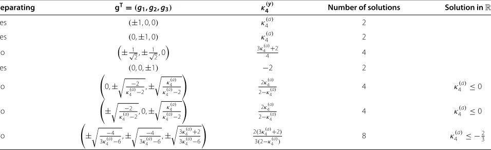
The corresponding system is polynomial. Using well-known algebraic techniques now implemented in many computer algebra systems [28], one can get a system of tri-angular equations equivalent to (7), whose solutions can be given explicitly. Forκ₄(a) = 2, there are 26 solutions to (7), some of them being complex-valued depending on κ₄(a). In Table 1, we give the real-valued solutions to (7) and the corresponding value ofκ₄(y). We also indicate for which values ofκ₄(a)the solutions hold.

For all values ofκ₄(a) =2 in Proposition 1 one can then consider all potential maxima in Table 1 and check which one maximizes|κ₄(y)|.

Forκ₄(a) = 2, thenκ₄(y) = 2(g₁2+g₂2)2−2g₃4and, using again the Lagrangian, it can be checked by hand that the extrema of κ₄(y) subject to g 2 = 1 satisfy eitherg1 =

g2=0,g23=1 org12+g22=1,g3=0.

Amazingly, the above result does not hold any longer if one considers a mixture of only the ﬁrst two components of the sources given by AssumptionA1.

Proposition 2.Let y = gswhere the vector of sources is given by the ﬁrst two components s = (s1,s2)T of

the sources deﬁned by A1. The function in Equation (5) satisﬁes:

• Ifκ₄(a)<−₇2orκ₄(a)>2, it is a contrast function and its maximization leads to extraction of eithers1ors2

(that is:g=(±1, 0)org=(0,±1)),

• if−2₇≤κ₄(a)≤2, it is not a contrast function and its maximization leads to a non-separating solution of the typeg=(±√1

2,±

1

√

2).

Table 1 List of all 26 solutions to Equation (7) forκ₄(a)=2 (second column), corresponding value ofκ₄(y)(third column) and condition for the solution g to be real-valued (last column)

(5)

Proof.The proof is similar to the proof of Proposition 1. Indeed, we haveκ₄(y)=κ₄(a)(g4

1+g24)+

κ₄(a)+2g₁2g₂2and

the Lagrangian readsL=κ₄(a)(g₁4+g₂4)+

κ₄(a)+2g₁2g2₂−

λ(g2₁+g₂2−1). Using a computer algebra system, one can then check that (7) is satisﬁed at 8 points. These points correspond to values of(g1,g2) andκ₄(y)which are given

in the ﬁrst three rows of Table 1 (precisely those rows for whichg3=0). Then, (5) is a contrast function if and only

if its maximization yields a separating solution, that is if

and only if|κ₄(a)|>|3κ (a)

4 +2

4 |. The proposition then follows

easily.

3.2 Pairwise and mutual independence

3.2.1 Pairwise independent sources

We now investigate the particular case of pairwise inde-pendent sources and introduce the following source vec-tor:

A2. s=(s1,s2,s3,s4)Twheres1,s2ands3are

independent BPSK ands4=s1s2s3.

This case has been considered in [20], where it has been shown that

∀i∈ {1,. . ., 4}, Cum {si,si,si,si} = −2 , (8)

Cum {s1,s2,s3,s4} =1

and all other cross-cumulants vanish. The latter cumu-lant value shows that the sources are mutually dependent; although it can be shown that they are pairwise indepen-dent. It should be clear that pairwise independence is not equivalent to mutual independence but in an ICA context, it is relevant to recall the following proposition, which is a direct consequence of Darmois’ theorem ([25], p. 294):

Property 1.Let s be a random vector with mutually independent components, andx = Gs. Then the mutual independence of the entries of x is equivalent to their pairwise independence.

Based on this proposition, the ICA algorithm in [25] searches for an output vector with pairwise independent components. Let us stress that this holds only if the source vector hasmutually independent components: pairwise independence is indeed not suﬃcient to ensure identiﬁa-bility as we will see in following section.

3.2.2 Pairwise independence is not suﬃcient

We ﬁrst have the following preliminary result:

Lemma 3.Let y = gs where the vector of sources is deﬁned byA2. Assume that the vector(s1,s2,s3)takes all23

possible values. If the signal y has values in{−1,+1}, then g=(g1,g2,g3,g4)is either one of the solutions below:

_∃_i_{∈ {}_1,

. . ., 4} gi= ±1, and: ∀j=i,gj=0

∃i∈ {1,. . ., 4} gi= ±1/2, and: ∀j=i,gj= −gi

(9)

Proof.If y = gs, using the fact that s2_i = 1 fori = 1,. . ., 4, we have with the particular sources given byA2:

y2=g2₁+g₂2+g₃2+g₄2

+2g1g2+g3g4

s1s2+

g1g3+g2g4

s1s3

+g2g3+g1g4

s2s3

Since (s1,s2,s3) take all possible values in {−1, 1}3, we

deduce from y2 = 1 that the following equations necessarily hold:

g₁2+g₂2+g2₃+g₄2=1

g1g2+g3g4=g1g3+g2g4=g2g3+g1g4=0

(10)

First observe that values given in (9) indeed satisfy (10). Yet, if a polynomial system ofNequations of degreedinN variables admits a ﬁnite number of solutionsb, then there can be at mostdNdistinct solutions. Hence we have found them all in (9), since (9) provides us with 16 solutions for (g1,g2,g3,g4).

Using the above result, we are now able to specify the output of classical ICA algorithms when applied to a mixture of sources which satisfyA2.

Constant modulus and contrasts based on fourth order cumulants The constant modulus (CM) criterion is one of the most known criteria for BSS. In the real valued case, it simpliﬁes to:

JCM(g)E

y2−12

with: y=gs (11)

Proposition 3.For the sources given by A2, the mini-mization of the constant modulus criterion with respect to gleads to either one of the solutions given by Equation (9).

Proof.We know that the minimum value of the con-stant modulus criterion is zero and that this value can be reached (forghaving one entry being±1 and other entries zero). Moreover, the vanishing of the constant modulus criterion implies thaty2−1=0 almost surely and one can then apply Lemma 3.

A connection can now be established with the fourth-order auto-cumulant if we impose the following constraint:

(6)

Because of the scaling ambiguity of BSS, the above nor-malization can be freely imposed. Under (12), we have κ₄(y) = Ey2₋₁2 ₋_{2 and minimizing} _J

CM(g) thus

amounts to maximizing−κ₄(y). Unfortunately, since κ₄(y) may be positive or negative, no simple relation between

|κ₄(y)|andJCM(g)can be deduced from the above equation.

Recall that usual results on contrasts do not apply here since source s4 depends on the others ([1], pp. 83–85).

However, we can state:

Proposition 4. Let y=gswhere the vector of sources is deﬁned byA2. Then, under the constraint (12) ( g = 1), we have:

(i) The maximization ofg→ −κ₄(y)leads to either one of the solutions given by Equation (9).

(ii)|κ₄(y)| ≤2and the equality|κ₄(y)| =2holds true if and only ifgis one of the solutions given in Equation (9).

Proof. Part (i) follows from the arguments given above. In addition, using multilinearity of the cumulants and (8), we have fory=gs:

κ₄(y)= −2g₁4+g₂4+g₃4+g4₄+24g1g2g3g4

(13)

The result then follows straightforwardly from the study of the polynomial function in Equation (13). Indeed, opti-mizing (13) leads to the following Lagrangian:

L= −2

After solving the polynomial system which cancels the Jacobian of the above expression, one can check that all solutions are such that |κ₄(y)| ≤ 2. Part (ii) of the proposition easily follows.

3.3 Simulations

3.3.1 Context

We illustrate with a few simulations Propositions 1 and 2. The random variable a in Assumption A1 has been generated as the following mixture of Gaussians:

a∼ 1

We generated mixtures of the sources given by Assump-tionA1: we mixed the three sourcess1,s2,s3 or the two

sourcess1,s2only with a matrixArandomly generated in

R3×3_or_R2×2_{, respectively.}

3.3.2 Algorithm

We used the algorithm CoM2 described in [25] and ([1], Chap. 5). It relies on the following MIMO extension of criterion (5):

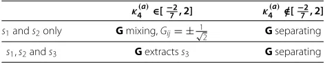
The algorithm in [25] ﬁrst operates a prewhitening and the maximization of the above criterion is performed over the set of orthogonal matrices. From the results of Propo-sitions 1 and 2 we expect the separation results which are given in Table 2, depending onκ₄(a) and the number of mixed sources. In Table 2, G is said separating when Above, Gis said separating when G = PD where P is a permutation matrix and D = diag(±1,. . .,±1) and

We provide some results illustrating Propositions 1 and 2 through the behavior of the algorithm CoM2. Let us deﬁne the following performance criterion: sourcekis well separated.

We performed 100 Monte-Carlo runs both in the case where the three sources A1 and in the case where only s1,s2 are mixed. The average results are provided in

Tables 3 and 4. We see in Table 3 thatτ3 is small in all

cases, indicating that the sources3is indeed separated by

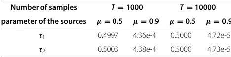
the algorithm. On the contrary, one can see in Tables 3 and 4 thatτ₁,τ₂are small only forμ = 0.9: this corresponds to a value ofκ₄(a)for which the obtainedGis theoretically separating. On the contrary, forμ = 0.5, corresponding to a value ofκ₄(a)for which the obtainedGdoes not theo-retically separates1ands2, the values ofτ1andτ2are close

to 0.5.

Table 2 Separation result provided by CoM2 for dependent sources satisfying A1

(7)

Table 3 Separation results of randomly driven mixtures of the three sources given by Assumption A1, average values over 100 Monte-Carlo runs

Number of samples T=1000 T=10000

parameter of the sources μ=0.5 μ=0.9 μ=0.5 μ=0.9

τ1 0.4995 0.0109 0.5000 0.0051

τ2 0.5001 0.0161 0.5000 0.0051

τ3 0.0117 0.0053 2.80e-4 2.76e-5

4 Extended ICA model

We have seen that, depending on the value of κ₄(a), the classical optimization criteria in Equations (5) and (16) are not contrasts any longer for the first two sources given by AssumptionA1. We now introduce a new statistical model of dependent sources, which consists in a probability mix-ture of sources. One component of the probability mixmix-ture satisfies the requirement of ICA, whereas the other com-ponent of the probability mixture is dependent. As an interesting example of dependent sources, we will con-sider the first two sources defined byA1, whereais the mixture of Gaussians proposed in Section 3.3 withμ = 0.5: this choice is justified by the previous results, which state that such sources cannot be separated by classical algorithms. We show that for our model, the separation is possible based on ICA and on the subset of samples where ICA assumptions are satisfied.

4.1 Latent variables

We ﬁrst extend ICA methods and relax the independence assumption. The basic idea consists in introducing a hid-den process r(t) such that, depending on the particular value of r(t) at instantt, the independence assumption is relaxed at timet. In this article, we will assume that r(t) can take two values only in the set {0, 1}. Let r (r(1),. . .,r(T)). We assume more precisely:

A3.Conditionally onr, the components

s(1),. . .,s(T)ofSat diﬀerent times are independent and for allt∈ {1,. . .,T}we have

P(s(t)|r)=P(s(t)|r(t)).

A4.Conditionally onr(t), whenr(t)=0, the components ofs(t)are mutually independent and non Gaussian, except possibly one of them;

Table 4 Separation results of randomly driven mixtures of mixtures of the ﬁrst two sources(s1,s2)given by

Assumption A1, average values over 100 Monte-Carlo runs

Number of samples T₌1000 T₌10000

parameter of the sources μ₌0.5 μ₌0.9 μ₌0.5 μ₌0.9

τ1 0.4997 4.36e-4 0.5000 4.72e-5

τ2 0.5003 4.38e-4 0.5000 4.73e-5

A5.Conditionally onr(t), whenr(t)=1, the components ofs(t)are dependent.

One can see that, conditionally onr(t) = 0, the source componentss(t)at time tsatisfy the usual assumptions required by ICA. In a BSS context, if r were known, one could easily apply ICA techniques by discarding the time instants where the sources do not satisfy the ICA assumptions. To be more precise, let us deﬁne:

I0{t∈ {1,. . .,T} |r(t)=0} (17)

and: X0(x(t))t∈I0 (18)

The setI0is the set of time instants where the

compo-nents ofs(t) are independent and non Gaussian, except possibly one of them. Then the subset X0 of the whole

setXof the observations satisﬁes the assumptions usually required by ICA techniques. The core idea of our method consists in performing alternatively and iteratively an esti-mation of B (corresponding toA−1) and of the hidden datar.

4.2 Typical sources separated by the proposed method The sources that we consider satisfy AssumptionsA3.,A4., and A5.given previously in Section 4.1. We now detail our particular choices forA4.,A5., which have been used in simulations and in the sequel to illustrate the assump-tions. These particular choices are denoted hereunder by A4.’ andA5.’ orA5.”.

We have considered two particular examples withN=2 sources. In both cases, AssumptionA4.particularizes to:

A4.’ Whenr(t)=0, the components ofs(t)are mutually independent, uniformly distributed on [−√3,√3](that is: zero-mean and unit variance).

4.2.1 Example 1

As a ﬁrst example, we particularize Assumption A5.as follows:

A5.’ Whenr(t)=1, thens1(t)=a(t)and

s2(t)=(t)a(t), where(t)is an independent BPSK

random variable anda(t)is an independent zero-mean, unit-variance random variable.

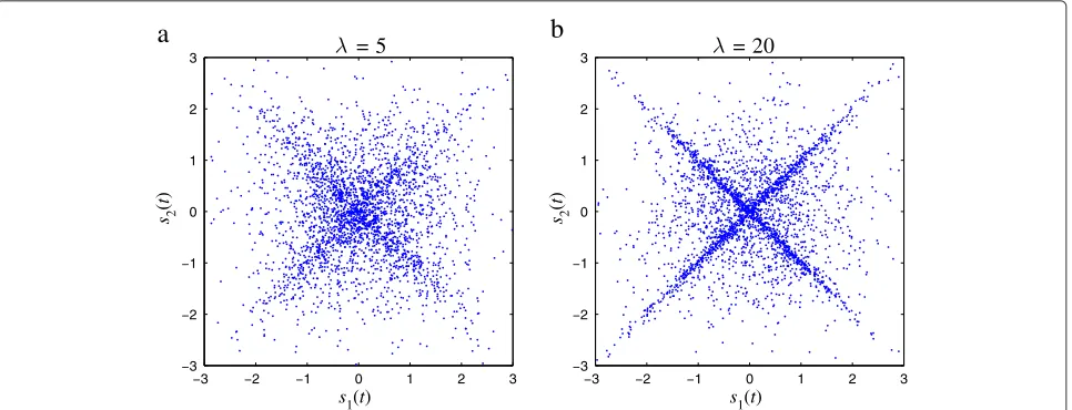
In simulations, we choosea(t)as a mixture of Gaussians whose distribution is given in Equation (15). A typical realization of a distribution satisfying A3., A4.’ andA5.’ is illustrated by the simulated values shown in Figure 1a. Conditionally onr(t)=1, the vector(s1(t),s2(t))T

corre-sponds to the ﬁrst two sources in AssumptionA1, which means that for r(t) = 1, (s1(t),s2(t))T lie on one of

(8)

0 1 2 3 0

1 2 3

s2

(

t

)

s₁(t) x₁(t)

sources

0 1 2 3

−3 −2 −1

−3 −2 −1 −3 −2 −1

0 1 2 3

x2

(

t

)

observations

a

b

Figure 1Typical density plot of the sourcessin example 1(a)and corresponding observationsx=As (b).

functions (such as CoM2) should not separate any lin-ear mixture of(s1(t),s2(t))T based on the samples where

r(t)=1.

On the contrary, considering the samples X0 only

amounts to removing the set of dependent points that lie on the two bisectors of Figure 2a. In such a case, the remaining samples inX0satisfy the usual requirement for

ICA and any ICA algorithm should succeed in separating a linear mixture of the sources.

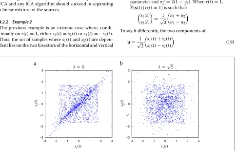
4.2.2 Example 2

The previous example is an extreme case where, condi-tionally onr(t)=1, eithers1(t)=s2(t)ors1(t)= −s2(t).

Thus, the set of samples wheres1(t)ands2(t)are

depen-dent lies on the two bisectors of the horizontal and vertical

axes. We considered in this example the case where, con-ditionally on r(t) = 1, the components of (s1(t),s2(t))T

are dependent but have a continuous joint density. We particularize AssumptionA5.as follows:

A5.” Letu1∼N(0,σλ)and:u2∼L(λ)be

independent random variables whereλis a positive parameter andσ_λ2=2(1−_λ12). Whenr(t)=1, P(s(t)|r(t)=1)is such that:

$ s1(t)

s2(t)

% = √1

2 $

u1+u2

u1−u2

%

To say it diﬀerently, the two components of

u= √1 2

$

s1(t)+s2(t)

s1(t)−s2(t)

%

(19)

−3 −2 −1 0 1 2 3

s₁(t) s₁(t)

s2

(

t

)

a

−3 −2 −1 0 1 2 3

s2

(

t

)

b

(9)

are independent, the ﬁrst one being Gaussian and the sec-ond one being Laplace distributed. One can verify that the choice ofσ_λ2ensures that, conditionally onr(t) = 1, the sources are unit-variance. Such a distribution density is illustrated by simulated values in Figure 2a withλ=5 and in Figure 2b withλ = √2. ConsideringX0only amounts

to removing the cloud set of dependent points on the distributions. Visually, this seems much more difficult in Figure 2b than in Figure 2a, and much more difficult in this example than in Example 1 in Figure 1a. We will discuss further in Section 7 the influence of a good knowledge of r: surprisingly, it is not necessarily crucial in our method to have a good knowledge ofr.

5 Separation method for the extended ICA model

5.1 Complete and incomplete data

Let us denote byθ = (B,η) the set of parameters to be estimated from the data: in this notation, we stress that θ consists of the separating matrixBand of the parame-ter vectorηwhich characterize the distribution of r. Let us call(r,X)the set ofcompletedata, whereasXalone is the set ofincompletedata: sinceris a hidden process, the model described in Section 4 corresponds to the situa-tion where only incomplete data is available for estimasitua-tion of the searched parameters θ. Note that the adjective blindis used to emphasize thatSis unavailable, whereas incompleteemphasizes thatris unavailable.

5.2 Iterative conditional estimation

Iterative conditional estimation (ICE) is an iterative esti-mation method that applies in the context of incomplete data and that has been proposed in the problem of image segmentation [24,29,30].

Another well-known iterative estimation technique is the expectation-maximization (EM) algorithm, which is based on the maximum likelihood estimator. Contrary to EM, the underlying estimator in ICE can be of any kind. This makes ICE more widely applicable in cases where the likelihood computation or maximization becomes intractable [29,31], for example in the non gaussian case. In the case where the maximum likelihood is chosen as the underlying estimator, ICE show similarities with EM (see e.g., [32] for an experimental comparative study). It has been proven in [33] that in the case of distributions belonging to the exponential family, EM is one particular case of ICE. Finally, the interest of ICE and its convergence in the case of data that are probability mixtures has been showed in [34].

We now shortly describe ICE. The prerequisites in order to apply ICE are the following:

• there exist an estimator from complete dataθ (ˆ r,X), • one is able either to calculateE{ ˆθ (r,X)|X;θ}or to

draw random variables according toP(r|X;θ ).

Starting from an initial guess of the parameters, the method consists in finding iteratively a sequence of esti-mates ofθ, where each estimate is based on the previous one. More precisely, ifθˆ[0]is the first guess, the sequence of ICE estimates is defined by:

ˆ

θ[q]=E{ ˆθ (r,X)|X;θˆ[q−1]}, (20)

whereE{. |X;θˆ[q−1]}denotes the expectation condition-ally onXand with parameter valuesθˆ[q−1]. If the above conditional expectation cannot be computed, it can be replaced by a sample mean, that is (20) can be replaced by:

ˆ

θ[p]= 1 K

K

k=1

ˆ

θ (r(k),X), (21)

whereK∈N∗is ﬁxed and eachr(k)_{is drawn according to} the a posteriori lawP(r|X;θˆ[q−1]). Note that ifθis vector-valued, (20) can be used for those components for which it can be computed, and (21) can be used otherwise.

Remark that the two conditions requested in order to apply ICE are very weak, which is the reason for our interest in ICE. In fact concerning the ﬁrst one, there would be no hope to perform incomplete data estimation if no complete data estimator exists, whereas the sec-ond requirement consists only in being able to simulate random values according to the a posteriori law.

5.3 Applicability of ICE and assumed distributions In this section, we give details about how the two condi-tions given in 5.2 for applicability of ICE are fulﬁlled.

First, as explained in Section 4.1, knowingrprovides an easy way of estimating a separating matrix by considering as in (18) the subsetX0of the samples. A complete data

estimatorθ (ˆ r,X)hence exists.

To use ICE, one should additionally know the law P(r|X;η). SinceX=AS, we have

P(r|X;η)= P(r,X;η) P(X;η) =

P(r,S;η)

P(S;η) (22)

(10)

AssumptionA3.only, the joint distribution of(r,S)under the parameter valueηreads:

P(r,S;η)=P(r;η)

T

t=1

P(s(t)|r(t);η) (23)

The above equation holds both for the assumed distribu-tion and for the distribudistribu-tion of the simulated data. On the contrary, the expressions ofP(r;η)andP(s(t)|r(t);η)that are assumed in ICE diﬀer from the ones of the simulated data and they are given in the next paragraphs.

5.3.1 AssumedP(s(t)|r(t))in ICE

First, note that in the following, similarly to the real data distribution,P(s(t)|r(t);η) = P(s(t)|r(t))does not depend on the parametersηto be estimated.

Experimentally, we observed that, for robustness rea-sons, the distributionP(s(t)|r(t))assumed in ICE should not have a bounded support or be too speciﬁc. For this reason, we assumed the following distributions:

• P(s(t)|r(t)=0)∼N(0, 1),

• P(s(t)|r(t)=1)is such that both components ofu deﬁned in (19) have the distribution

1

2L(λ)+ 12N

0,σ_λ2.

A typical realization of the distribution of(s1(t),s2(t))T

assumed in ICE is given in Figure 3. This distribution is of course diﬀerent from the ones of the simulated data in Figures 1 and 2. However, simulations will conﬁrm that it is a reasonable choice.

Conditionally on r(t) = 0, (s1(t),s2(t))T is assumed

an independent, zero-mean, unit-variance Gaussian vec-tor: this is an uninformative distribution having a density with non bounded support. Conditionally on r(t) = 1,

each component ofuin the assumed distribution is a mix-ture of a Laplace and a Gaussian law. Experimentally, and from the observation of Figures 1 and 3, the latter choice seems a relevant approximation of the data model from Example 1 in Section 4.2.1. The parameterλshould make a compromise between a good ﬁt to the data (λlarge) and robustness of the method (λ small). Also, the assumed conditional distributionP(s(t)|r(t)=1)is invariant with respect to any permutation and sign change. Such a sym-metry is necessary in our method because ICA algorithms leave permutation ambiguities. For this reason, the same distribution has been considered to model the data source signals generated in Example 2 (Section 4.2.2).

5.3.2 AssumedP(r;η)in ICE

We propose two diﬀerent models for the latent processr. I.i.d. latent process

The simplest case is whenris an i.i.d. Bernoulli process, that isηis a scalar parameter in [ 0, 1] and:

P(r;η)=

T

t=1

P(r(t);η) (24)

with for allt∈ {1,. . .,T}:

P(r(t)=0)=η and P(r(t)=1)=1−η (25)

Markov latent process

We can alternatively consider that r is a stationary Markov Chain, that is:

P(r)=P(r(1))

T

t=2

P(r(t)|r(t−1)),

where P(r(t)|r(t − 1)) is given by a transition matrix independent oft. In this case, the parameters ηconsist

3 2 1 0 1 2 3

s₁(t) s2

(

t

)

= 5

3 2 1 0 1 2 3

s₁(t) s2

(

t

)

= 20

a

b

(11)

of the diﬀerent transition probabilities and the ini-tial probabilities. The main advantage of consider-ing a Markov model is that the posterior transitions P(r(t)|r(t − 1),X;η) can be calculated by an eﬃ-cient forward-backward algorithm [35]. A sampling of the hidden process according to the posterior law P(r|X;η) is hence possible, making the ICE method applicable [29].

6 Combined ICA/ICE separation algorithm

In this section, we ﬁrst detail our separation algorithm which combines ICA and ICE. We then interpret ICE in terms of random variable generation.

6.1 Algorithm

We denote byICAone among all possible ICA algorithms [1] such as JADE [26], CoM2 [25], FastICA [27], etc. Given a set of observation samplesX, the separating matrix esti-mated by the ICA algorithm is denoted byB= ICA(X). With these notations, a complete data estimator of the separating matrix is provided byB=ICA(X0), whereX0

has been deﬁned in Equation (18). Our algorithm consists in an ICE estimation of the parametersθ = (B,η). The parametersηwhich characterizerare estimated accord-ing to (20), whereas the separataccord-ing matrixBis estimated according to (21) withK = 1. Here is a summary of the algorithm:

Initialize the parametersθˆ[0] =

ˆ

B[0],ηˆ[0]

. Forq = 1, 2,. . .,qmax, repeat:

1. calculateP

r|X;θˆ[q]

and drawrˆ[q]according to this distribution,

2. update the separating matrix:

• set:Iˆ₀[q]=t| ˆr[q](t)=0and ˆ

X[₀q]=(x(t))

t∈ ˆI[q] 0 • ˆB[q+1]=ICA

ˆ

X[₀q]

.

3. update the parametersηof the processr.

Steps 1 and 3 of the above algorithm are further detailed in the following sections. Note that, if the parametersη are available as an additional information, they need not be estimated and step 3 of the algorithm is not necessary.

6.2 Details in the case of an i.i.d. latent process

We here detail the three steps of our algorithm in the case whereris i.i.d. As we will see, in this case, ICE is akin to generating a set of random samples that satisfy the usual assumptions of ICA with an accept-reject method.

6.2.1 Step 1

In the case whereris i.i.d., we have from (22), (23), and (24):

P(r|X;η)=

T

t=1

P(r(t);η)P(s(t)|r(t)) P(s(t))

= T

t=1

P(r(t)|s(t);η),

where P(r(t);η) has been given in Equation (25) and P(s(t)|r(t))has been described in Section 5.3.1. Writing αt = P(r(t) = 0|X;η)(and hence 1−αt = P(r(t) = 1 |X;η), it follows from the above equation that in step 1, all samples ofˆr[q]are independent and such that

ˆ

r[q](t)=0 with probability α_t

ˆ

r[q](t)=1 with probability 1−αt.

6.2.2 Step 2: accept-reject random variable generation

One can see that, when selectingXˆ[₀q]in the second step of our algorithm, some samples are kept, others are thrown away. A close parallel can be drawn with random variable generation by the acceptance-rejection method.

For clarity, let us deﬁneP0(s(t))=P(s(t)|r(t)=0)and

P1(s(t))= P(s(t)|r(t) = 1). At timet, according also to

Equations (25) and (23), the distribution ofs(t)is given by:

ηP₀(s(t))+(1−η)P₁(s(t))

We have the following lemma:

Lemma 4.Letsbe a random variable (or random vector) with probability distribution given by

s∼ηP0(s)+(1−η)P1(s)

Letˆr∈ {0, 1}be a binary random variable with probability distribution such that:

P(ˆr=0|s)= ηP0(s)

ηP₀(s)+(1−η)P₁(s) (26)

P(ˆr=1|s)= (1−η)P1(s) ηP0(s)+(1−η)P1(s)

(27)

Then, the conditional distributionP(s| ˆr=0)isP0(s).

Proof.One can write the joint probability distribution P(s,rˆ) =ηδ(ˆr=0)P0(s)+(1−η)δ(rˆ= 1)P1(s)and the

result follows by conditioning.

(12)

distributionP0(s)is generated using the instrumental

dis-tribution g(s) = ηP0(s) +(1− η)P1(s). Samples from

this instrumental distributiong(s) are given by the data themselves. By doing so, we obtain a set of data following the distributionP0(s). SinceP0(s(t))= P(s(t)|r(t) = 0)

and according to Assumption A4., this is precisely the distribution under which the ICA algorithm is applicable.

Remark 3. It is known that the probability distribution of s in Lemma 4 can be seen as the marginal of (r,s), whereris a Bernoulli process and the conditional laws of sknowingrare given byP0andP1. However,rˆis drawn

independently ofrand in particular,rîs different fromr. It means that in our algorithm, the original latent processr and the ICE samplingrˆ[q]may be quite different, although the selected samples are distributed followingP0. This will

be illustrated in Section 7.1.2.

6.2.3 Step 3

A complete data estimator of the parameter η is given by the empirical frequency ηˆ = _T1#T_t₌₁δ(r(t) = 0). Equation (20) then yields the following update rule for the parameterη:

ˆ

η[q+1]= 1 T

T

t=1

Pr(t)=0|x(t),θˆ[q] (28)

6.3 Markov latent process

We here detail the three steps of our algorithm in the case whereris a Markov process.

6.3.1 Step 1

Here, we assume in the ICE part of the procedure that r is a Markov process. Then, the posterior probability P(r|X;θˆ[q])is Markov, and its transitions can be calcu-lated according to the forward-backward or Baum-Welch algorithm. At each step q of the algorithm, rˆ[q] is then generated according to P(r|X;θˆ[q]) as a non-stationary Markov chain. It is out of the scope to further detail these well-known procedures and the reader is referred to [29,30,35] and references therein for more explanations.

6.3.2 Step 2

It is unchanged, although the interpretation as an accept-reject random variable generation does not hold any longer.

6.3.3 Step 3

From the values of P(r(t)|X,θˆ[q]) and P(r(t),r(t + 1))

|X,θˆ[q]), formulas similar to Equation (28) yield the esti-mated probabilities forr(t)and the pairs(r(t),r(t+1)). The transition probabilities are then obtained by the rela-tionP(r(t +1))|r(t),X,θˆ[q]) = P(r(t),r(t+1))|X,θˆ[q])

P(r(t)|X,θˆ[q]) . The reader is again referred to [29,30,35] for more details.

7 Simulations

We performed several simulations for diﬀerent numbers of samples, respectively,T=1000,T=5000,T=10000. We have setqmax = 30 in our algorithm: this value has

been determined empirically by testing values ofqmaxup

to 150. For values greater thanqmax = 30, no signiﬁcant

quality improvement has been observed and this choice seems hence satisfactory as far as ICE convergence is con-cerned. Although highly interesting, a more detailed anal-ysis of the convergence speed/rate of our algorithm is out of the scope of the article. The separation quality criterion considered is the mean square error (MSE): the provided value is a mean of the MSE over all sources. Additionally, we considered the empirical segmentation rate provided by the last samplingrˆ[qmax]_{in Step 1 of the ICE procedure.} We deﬁne this segmentation rate as follows:

ϒICE=

1 T

T

t=1

δ

ˆ

r[qmax]₍_t₎=_r₍_t₎_. ₍₂₉₎

This corresponds to the proportion of time samples which are correctly classiﬁed as corresponding either to independent (r(t)=0) sources or to dependent (r(t)=1) sources. In all cases, the source signals and the mixing matrix have been randomly generated.

The classical algorithm used in our simulations, which has been denotedICAin Section 6 was CoM2 [25]. For comparison, we considered as a worst case reference the result when CoM2 is applied to the data, simply ignor-ing that the ICA assumptions are violated at some sample times. On the other hand, as an optimal best case refer-ence, we considered the complete data situation, that is whenris available and the separation is performed based onX0.

In our simulations, we generated data according to the following models:

• sources satisfyingExample 1in Section 4.2. We chose the processa(t)as a mixture of Gaussians as deﬁned in Equation (15), withμ=0.5. According to Section 3, the CoM2 algorithm, if applied on the dependent data only, is not successful in separating the sources.

• sources satisfyingExample 2in Section 4.2. In this case, we chooseλ=√2.

7.1 I.i.d. latent process with knownη

We ﬁrst provide some simulations in the case whereris an i.i.d. Bernoulli process with knownη parameter (see Equation (24)).

7.1.1 Example 1

(13)

0 0.2 0.4 0.6 0.8 1 104

103 102 101 100

Average MSE

a

ICE + CoM2 r+CoM2 CoM2

0 0.2 0.4 0.6 0.8 1

0.7 0.8 0.9 1

Average ICE

0 0.2 0.4 0.6 0.8 1

105 104 103 102 101 100

Average MSE

b

0 0.2 0.4 0.6 0.8 1

0.7 0.8 0.9 1

Average ICE

0 0.2 0.4 0.6 0.8 1

105 104 103 102 101 100

Average MSE

c

a

b

c

0 0.2 0.4 0.6 0.8 1

0.7 0.8 0.9 1

Average ICE

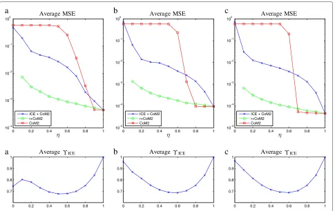
Figure 4Depending onη(known by the algorithm), average MSE and segmentation rateϒICE.Sources generated from Example 1 withr

i.i.d., parameterλ=5.(a)T=1000 samples,(b)T=5000 samples,(c)T=10000 samples.

Monte-Carlo realizations whereas values in Figure 5 are the individual results for 100 Monte-Carlo realizations.

In Figure 4, the MSE values have been plotted depending onη∈[ 0, 1] forT = 1000 (a),T = 5000 (b),T = 10000 (c) samples. Note that forη = 0, all samples of the data sources are dependent and the complete data separation is therefore not applicable. Similarly, when settingηto zero in the ICE algorithm, all samples are necessarily classi-ﬁed as dependent and our method is not applicable. For this reason, whenη = 0 has been used in the simulated sources we have setηto 0.1 in the algorithm.

Naturally, the complete data case provides the best results: whenηtends to zero, the number of samples inX0

decreases, which explains the increasing MSE for smaller η values. On the other hand, ignoring the dependence provides results that are unacceptable forηsmaller than 0.7, approximately. It seems however that CoM2 is able to separate the particular sources considered forηgreater then 0.7, approximately: from the results in Section 3, the existence of such a limit value above which CoM2 is successful seems quite natural. Forηsmaller than 0.7 the proposed method provides a very signiﬁcant improve-ment in terms of separation quality. The classiﬁcation rate ϒ_ICEhas also been plotted in Figure 4 and one can observe that samples of dependent/independent sources are quite

well classiﬁed, which corroborates the good MSE values obtained with our method.

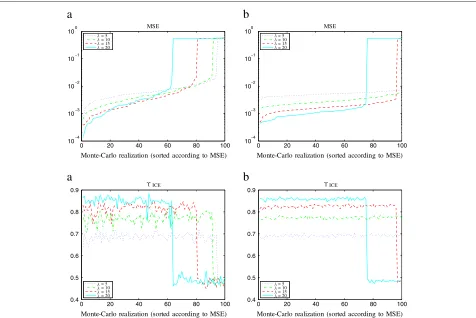
Depending on the parameter λ, the source distribu-tion assumed in the ICE estimadistribu-tion and described in Section 5.3.1 is closer to or farther from the real source distribution of Example 1, which has part of its samples lying on the two bisectors (see the comparison between Figure 1a and Figure 3a,b). In Figure 5, we tested the inﬂu-ence of the parameterλfor a ﬁxed value ofη= 0.5. The MSE of 100 Monte-Carlo realizations have been plotted forT = 1000 andT = 10000 samples. The correspond-ing segmentation rateϒICEhas been plotted in the lower

part of the ﬁgures. First, it can be seen in Figure 5 that the separation results of the Monte-Carlo realizations can be clearly separated in two groups:

• for a minority of cases, the segmentation rateϒICEis close to 0.5, meaning that the procedure completely fails to classify the latent processr. In such a case, the corresponding MSE is important (around0.5) and separation is unsuccessful. This situation occurs more often for large values ofλ: a greater value ofλ

consequently implies less robustness of our method. • for most of the realizations,ϒ_ICEis signiﬁcantly

(14)

0 20 40 60 80 100 104

103 102 101 100

Monte-Carlo realization (sorted according to MSE)

MSE

a

= 5 = 10 = 15 = 20

0 20 40 60 80 100

0.4 0.5 0.6 0.7 0.8 0.9

ICE

= 5 = 10 = 15 = 20

0 20 40 60 80 100

104 103 102 101 100

MSE

b

a

b

= 5 = 10 = 15 = 20

0 20 40 60 80 100

0.4 0.5 0.6 0.7 0.8 0.9

ICE

= 5 = 10 = 15 = 20

Figure 5For diﬀerent values ofλ, MSE of 100 Monte-Carlo realizations sorted by increasing values and corresponding segmentation rate ϒICE.Sources generated from Example 1 withri.i.d.η=0.5 (known by the algorithm),(a)T=1000 samples,(b)T=10000 samples.

succeeds in classifying approximately the latent processr. In such a case, the corresponding MSE is low and the separation is successful. One can see that, in such a case where the separation is successful, a greater value ofλcomes with a greaterϒICE, hence a better segmentation ofrand a lower MSE, hence a better separation quality.

In conclusion, the choice of λ should be a compromise between good separation quality (in case of success) and robustness in order to limit the rate of separation failure.

7.1.2 Example 2

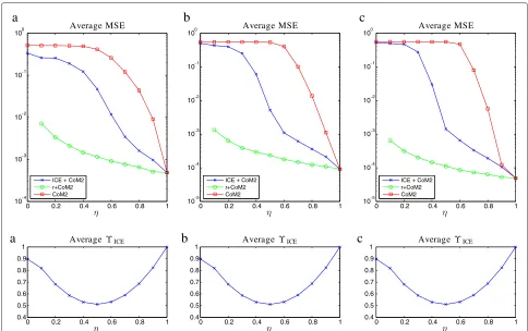
The results for source signals following Example 2 (see Section 4.2.2 withλ = √2) are given in Figure 6. Simi-larly to the previous section, forT =1000 (a),T = 5000 (b),T = 10000 (c) samples and depending onη ∈[ 0, 1] the MSE values have been plotted in the top graph and the segmentation rateϒ_ICEin the bottom graph.

As expected, the complete data estimation based onX0

of the separating matrix provides again the best results. In comparison with the case where the dependence of the sources is ignored, our method provides a very signiﬁ-cant improvement, in particular forηlying between 0.4

and 0.8, approximately. Very interestingly, as witnessed in Figure 6, the good performance in terms of separation and MSE is obtained with very poor performance in terms of classiﬁcation of the latent processr: note in particular that forη = 0.5, we have a low MSE whereasϒICE is close

to 0.5. The poor classification can be easily understood when comparing Figure 2b with Figure 1a. The important point in this observation is that a good classification of the latent processris a sufficient but not a necessary condi-tion for good ICA estimacondi-tion. This is in contrast with the former example but is fully justified by the interpretation of Step 2 of the algorithm in Section 6.2. Indeed, accord-ing to Lemma 4, the ICE part of our algorithm selects a set of samplesXˆ0which is such that its distribution

satis-ﬁes the usual ICA assumptions, although the classiﬁcation may well be very poor.

7.2 I.i.d. latent process with unknownη

(15)

0 0.2 0.4 0.6 0.8 1 104

103 102 101 100

Average MSE

a

0 0.2 0.4 0.6 0.8 1 0.4

0.5 0.6 0.7 0.8 0.9 1

Average ICE

0 0.2 0.4 0.6 0.8 1 105

104 103 102 101 100

Average MSE

b

0 0.2 0.4 0.6 0.8 1 0.4

0.5 0.6 0.7 0.8 0.9 1

Average ICE

0 0.2 0.4 0.6 0.8 1 105

104 103 102 101 100

Average MSE

c

a

b

c

0 0.2 0.4 0.6 0.8 1 0.4

0.5 0.6 0.7 0.8 0.9 1

Average ICE

Figure 6Depending onη(known by the algorithm), average MSE and segmentation rateϒICE.Sources generated from Example 2 withr

i.i.d. and parameterλ=√2.(a)T=1000 samples,(b)T=5000 samples,(c)T=10000 samples.

and Example 2. In the case of Example 1, we have set the parameter λ = 5 in the assumed distribution of Section 5.3.1, whereas we have setλ = √2 in the case of Example 2. For comparison, we provide the MSE results whenηis known and when the algorithm CoM2 is applied, just ignoring that the generated source signals are dependent.

One can see from the values in Table 5 that our sepa-ration method remains valid even in the case whereηis estimated.

7.3 Markov latent process

As previously indicated, the ICE estimation algorithm is able to take into account the Markov dependence of r.

We have considered the importance of modelingr as a Markov or i.i.d. process.

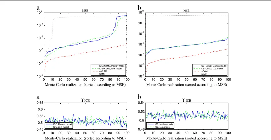
The process r has been generated as a stationary Markov chain with transition matrix 0.9 0.1_{0.1 0.9}, in which case P(r(t) = 0) = P(r(t) = 1) = 1₂. On the corresponding data set with r Markov, our separation method has been performed both in the case where r is modeled as i.i.d. and in the case wherer is modeled as a Markov chain. In both cases, the parameters in η have been estimated from the incomplete data. Figure 7 provides the results for sources from Example 1 (with λ = 15 in the algorithm) and Figure 8 provides the results for sources from Example 2 (with λ = √2 in the algorithm). The separation results with complete data

Table 5 Average MSE

Number of samples T₌1000 T₌5000 T₌10000

Parameterη 0.3 0.5 0.7 0.3 0.5 0.7 0.3 0.5 0.7

Example 1,ηknown 4.70e-2 2.70e-2 7.94e-3 1.04e-2 6.66e-3 2.59e-3 9.34e-3 5.42e-3 2.48e-3

Example 1,ηestimated 4.35e-1 8.17e-2 9.46e-3 5.36e-1 1.59e-2 4.59e-3 5.73e-1 8.50e-3 4.38e-3

Example 1, CoM2 5.86e-1 5.33e-1 3.62e-2 5.86e-1 5.84e-1 1.29e-3 5.86e-1 5.85e-1 5.43e-5

Example 2,ηknown 1.91e-1 4.71e-2 3.43e-3 2.51e-1 5.16e-3 6.15e-4 2.76e-1 1.42e-3 3.33e-4

Example 2,ηestimated 3.85e-1 6.66e-2 3.53e-3 5.43e-1 6.34e-3 6.60e-4 5.59e-1 1.77e-3 3.55e-4

Example 2, CoM2 5.04e-1 4.16e-1 1.20e-1 5.47e-1 5.38e-1 1.01e-1 5.57e-1 5.54e-1 7.99e-2

(16)

0 10 20 30 40 50 60 70 80 90 100 105

104 103 102 101

100 MSE

a

ICE+CoM2, Markov model ICE+CoM2, i.i.d. model r+CoM2 CoM2

0 10 20 30 40 50 60 70 80 90 100

0.4 0.6 0.8

1 ICE

a

ICE, Markov model ICE, i.i.d. model

0 10 20 30 40 50 60 70 80 90 100

106 105 104 103 102 101

100 MSE

b

0 10 20 30 40 50 60 70 80 90 100

0.4 0.6 0.8

1 ICE

b

Figure 7For an i.i.d.and a Markov model ofr, MSE of 100 Monte-Carlo realizations sorted by increasing values and corresponding segmentation rateϒICE. Sources generated from Example 1 withrMarkov,λ=15(a)T=1000 samples,(b)T=10000 samples.

and with CoM2 ignoring the dependence of the sources have also been plotted and, as expected, they correspond respectively to the best/worse MSE value. On the top plots of Figure 7, one can see that, in sources from Example 1, the performance is improved when taking into account

the Markovianity of r. More precisely, similarly to the simulations in Section 7.1.1 with λ = 15, the MSE values show a successful separation for a majority of real-izations: in such a case, the Markovianity assumption clearly improves the MSE. However, the Markovianity

0 10 20 30 40 50 60 70 80 90 100 105

104 103 102 101

100 MSE