Simulation of distant tsunami propagation with a radial loading deformation
effect
Daisuke Inazu and Tatsuhiko Saito
National Institute for Earth Science and Disaster Prevention, 3-1 Tennodai, Tsukuba, Ibaraki 305-0006, Japan
(Received October 29, 2012; Revised March 18, 2013; Accepted March 19, 2013; Online published September 17, 2013)
A simple parameterization of the loading deformation of the seafloor is incorporated into a tsunami simulation model in order to realistically calculate tsunami travel time, especially at regions far from the source. The parameterization uses one scalar parameter that is optimized effectively by far-field, deep-sea records of recent giant tsunamis: the 2011 Tohoku and the 2010 Chilean tsunamis. Using this parameterization with the optimal values, the observed tsunamis are realistically simulated in both near and far fields. The optimal values seem equivalent for both giant tsunamis, and are relatively smaller than those previously verified for ocean tide modeling, which is reasonable because of the shorter wavelengths of tsunamis.
Key words:Tsunami, travel time, self-attraction and loading.
1.
Introduction
Tsunami propagation has been simulated by long-wave (non-dispersive) equations, and this approximation has been applied to model observed tsunamis especially in near fields (e.g., Aida, 1969; Satake, 1985; Tsushima et al., 2011). Recently, trans-oceanic tsunami simulations, with travel distances exceeding thousands of kilometers, have re-ported apparent travel time differences between simulations and observations. The simulated travel times of the lead-ing tsunamis at regions further than 10000 km from their sources were systematically shorter than those of observa-tions by 15–20 minutes for cases of recent giant tsunamis generated by the 2004 Sumatra (Rabinovichet al., 2011), the 2010 Chilean (Katoet al., 2011; Fujii and Satake, 2013), and the 2011 Tohoku (Tanget al., 2012; Grilliet al., 2013) earthquakes. The leading wave of the simulated tsunamis by these ordinary tsunami models propagates with a phase velocity of√g Hwheregis the gravity acceleration andH is the water depth. We need to provide an appropriate mech-anism of the delayed propagation found in the observations and its advanced modeling.
Wave dispersion can make the phase velocity slower than the non-dispersive √g H. Two types of wave dispersion are suggested: in short wavelengths (<102km) and in long
wavelengths (>103km).
The phase velocity due to the short-wavelength
disper-sion is well known as
gtanh(k H)
k wherekis the
wavenum-ber. This wave dispersion arises as wave trains subsequent to the leading wave (e.g., Lamb, 1932; Takahashi, 1942; Kajiura, 1963; Saitoet al., 2010).
Meanwhile, interactions between an elastic Earth and
Copyright cThe Society of Geomagnetism and Earth, Planetary and Space Sci-ences (SGEPSS); The Seismological Society of Japan; The Volcanological Society of Japan; The Geodetic Society of Japan; The Japanese Society for Planetary Sci-ences; TERRAPUB.
doi:10.5047/eps.2013.03.010
a tsunami with long wavelengths have been theoretically predicted (Ward, 1980; Comer, 1984). The interactions can be recognized as another wave dispersion that arises from the elastic seafloor deformation due to the tsunami loading. The loading deformation produces a feedback on tsunami spatial patterns, and delays propagations of the leading tsunami with the longest wavelengths, as mentioned in the next section. Such a feedback is often called the ocean self-attraction and loading (SAL) effect (e.g., Ray, 1998).
It has been known that the SAL effect must be consid-ered for precise ocean tide modeling, especially for global modeling (e.g., Ray, 1998). Precise calculations of the SAL effect need convolutions of the global distribution of oceanic mass loading using spherical harmonics, Love numbers, and an Earth model (e.g., Farrell, 1972; Kantha and Clayson, 2000; Matsumotoet al., 2000), requiring rel-atively higher computational costs than ordinary tsunami models. On the other hand, the SAL effect can be mod-eled by a simple parameterization using one scalar param-eter (e.g., Accad and Pekeris, 1978; Parke, 1982) without a substantial increase in computational costs. This param-eterization yields less accurate results than the convolution method, but is better than modeling without any loading ef-fects. The SAL effects have been also implemented in mod-ern ocean general circulation modeling beyond the ocean tide (e.g., Stepanov and Hughes, 2004; Tamisiea et al., 2010).
The SAL effects have so far not been taken into account in tsunami propagation modeling. In the present study, a SAL effect is considered in a tsunami propagation model in order to examine the discrepancy of the simulated travel time. We implement a simple parameterization based on Accad and Pekeris (1978), and demonstrate that the pa-rameterization works to simulate realistic travel times and waveforms of near- and far-field tsunamis. The efficiency of
∂t = −g H∇(η−η0) , (1)
∂η
∂t + ∇ ·Q=0, (2)
η0=βη, (3)
whereQandηare the depth-integrated horizontal velocity and the tsunami height, respectively. g is the acceleration due to gravity (9.81 m/s2), and His the sea depth which is
given based on the ETOPO1 bathymetric dataset (Amante and Eakins, 2009). The SAL effect,η0, is added in the linear
long-wave equation.
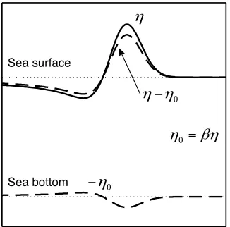
We apply a simple parameterization method using a con-stant scalar parameter (β) that has been used for classical ocean tide modeling (Accad and Pekeris, 1978; Ray, 1998). The representation indicates that radial (vertical) seafloor deformation is caused by only the loading above (Fig. 1). The phase velocity derived from Eqs. (1)–(3) is:
g H1−β. (4)
This shows that the tsunami propagation speed of the pa-rameterization is slower than√g H, and is non-dispersive. An empirical value ofβ = ∼0.1 has been sometimes used for ocean tide modeling (Ray, 1998; Kantha and Clayson, 2000). In the present study, the optimal β for tsunamis is empirically determined by tsunami records obtained by deep-sea ocean bottom pressure (OBP) gauges.
Tsunami simulations start from initial conditions given by the source models: A model with a moment magnitude
Fig. 1. Schematic of the SAL effect.η(solid) is the tsunami height without the SAL effect, andη0(dashed) is the SAL term.η−η0(dashed) is the
modified tsunami height.
shown in Fig. 2 are used for the respective tsunamis. KPG1 and MPG1 are operated by JAMSTEC, and other sites are DART stations.
4.
Validation of SAL Effect
Improving the horizontal resolution (10, 5, 2, and 1 ar-cmin) in the tsunami simulation is first confirmed to yield no substantial changes in the calculated travel times of the leading tsunami even in far fields (Fig. 3). The SAL effect is investigated using the finest resolution and bathymetry of 1 arcmin.
We examine different loading factors:β is tested within 0.000–0.040 for every 0.005. The simulated results are evaluated by the detided OBP data (Fig. 2). The accuracy of the simulations is measured by the root-mean-square (RMS) reduction of the observed tsunami for each OBP record. In the present study, the RMS reduction is evaluated at two-hour intervals containing the time when the leading tsunami reaches each OBP site, since the travel time is of focus. The RMS reduction is defined by a ratio of the residual RMS to the observed RMS:
RMSobserved-simulated
RMSobserved
. (5)
Significant RMS reduction is basically identified with max-imum correlation coefficients with a zero lag between the observation and simulation. The loading factor (β) is then optimized by the maximum RMS reduction.
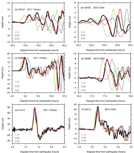
In the case of simulation with the loading factor ofβ = 0 (usual tsunami simulation), calculated travel times are shorter than observations, and the differences increase with distances from the source regions (Figs. 4 and 5(a)), as in-dicated by previous studies. Changingβ allows the calcu-lation of realistic travel times, especially in far fields, and hardly affects near-field travel times (Fig. 4).
Fig. 2. Locations of OBP data used for (a) the 2011 Tohoku (28 sites), and (b) the 2010 Chilean (20 sites) tsunamis. Stars denote the respective sources.
Fig. 3. Observed tsunami (black) and simulated results (colored) without the loading effect (β = 0) for different horizontal resolutions of the simulation (10, 5, 2, and 1 arcmin).
5.
Discussions on the Optimal
ββββββββ5.1 ββββββββand spatial scale of loading deformation
For ocean tide modeling, the optimal β was∼0.12 for diurnal constituents and∼0.08 for semidiurnal constituents (Parke, 1982; Ray, 1998). In general, the loading deforma-tion is significant for spatially large loading. Wavelengths of tsunamis are, at most, hundreds of kilometers and are shorter than those of ocean tides that are thousands of kilo-meters. Thus, deformation efficiency against tsunami load-ing is expected to be relatively weaker than that for ocean tide loading. The deformation efficiency is simply evalu-ated by a deformation equation of an elastic halfspace based on Jeffreys (1976),
d = (1−ν)
μk ρgη1coskx, (6)
whered is the vertical crustal deformation,μis the rigid-ity (30–40 GPa),ν is Poisson’s ratio (∼0.3), ρ is the sea-water density (1030 kg/m3), k is the wavenumber, and
ρgη1coskx is the applied pressure loading with a spatial
distribution in the horizontal (x) direction. Since we put
ρgη1coskx = ρgη and then d ≈ βη as the SAL
ef-fect in the present study, calculated wavelengths for the giant tsunamis (β = 0.015–0.020) are 400–700 km. The spatial scales seem reasonable and equivalent for the two tsunamis. It is also noted that, for example, a 1-m tsunami loading bearing such spatial scales generates an elastic, ver-tical seafloor deformation of 1.5–2.0 cm.
The difference between the phase velocities with, and without, the SAL effect is√g H1−√1−β ≈√g Hβ2, being 0.8–1.0% with the optimalβ. Meanwhile, the simu-lation without the SAL effect shows an apparent linear dis-crepancy for the travel time commonly for both tsunamis (Fig. 5(a)). The linear discrepancy agrees with the differ-ence of the phase velocities. The optimalβ common for both the tsunamis is also verified from Fig. 5(a), because the phase velocity represented by Eq. (4) indicates a linear deviation from√g H.
5.2 Effect of ocean density stratification onββββββββ
It has been mentioned above that the distant tsunami propagation is basically explained by the long-wave ap-proximation, i.e., a one-layer ocean model, and the elastic loading deformation. In a strict sense, it is known that the density structure of the real ocean contributes to the slow propagation of ocean gravity waves. So the optimalβ to some extent includes the effects of the density structure of the ocean as well. This effect is evaluated in this subsection. An ocean model that considers ocean stratification is nec-essary, in general, so as to represent realistic ocean circula-tions. Two-layer ocean models that are simplest, essential ones have been often used. The long-wave phase veloc-ity in a stratified ocean is revisited using a two-layer ocean model. A well known dispersion relation in the two-layer ocean model has been derived by Gill (1982) and Unoki (1993):
ω k
4
−g(h1+h2)
ω k
2
+εg2h1h2=0
ε=ρ2−ρ1
ρ2
, (7)
Fig. 4. Comparisons of observed tsunamis (black) with simulated results (colored) using differentβ(0.000, 0.020, and 0.040) at selected OBP sites. Left and right panels show the 2011 Tohoku and the 2010 Chilean tsunamis, respectively. These are typical examples in far (a, b), intermediate (c, d), and near (e, f) fields from the respective tsunami sources.
upper and lower layers in the two-layer ocean.h andρare the layer thickness and density of each layer, respectively. h1+h2 is the total depth. This equation yields two roots
as phase velocities of the surface gravity wave (C+) and the internal gravity wave (C−):
ω k
2
= 1
2g(h1+h2)
1± 1−4ε h1h2
(h1+h2)2
≈ 1
2g(h1+h2) ×
1±
1−2ε h1h2
(h1+h2)2 +
Oε2,(8)
C+=ω+
k ≈
g(h1+h2) 1−ε
h1h2
(h1+h2)2
C−=ω− k ≈ εg
h1h2
h1+h2
. (9)
C+ is mostly√g(h1+h2)because εis small, as little as
10−3in deep seas (e.g., Kindle and Thompson, 1989; Qiu,
2003; Pierini, 2006) and 10−2 in coastal seas (Gill, 1982;
Unoki, 1993).
Here, a deviation factor
1−ε h1h2
(h1+h2)2 is re-evaluated.
Table 1. Summary of the simulated results for (a) the 2011 Tohoku, and (b) the 2010 Chilean tsunamis at each OBP site. The results forβ∗(=0.015) are also shown.
(a) 2011 Tohoku tsunami
Site Latitude Longitude Depth Epicentral Travel Lag for RMS Optimal Lag for RMS
(◦N) (◦E) (m) distance time β=0 reduction β β∗ reduction
(km) (hr) (min) forβ=0 (min) forβ∗
21418 38.711 148.694 5663 552 0.5 −0.5 0.52 0.000 −0.5 0.55
21401 42.617 152.583 5264 987 1.1 0.0 0.35 0.000 −0.5 0.39
21413 30.515 152.117 5825 1246 1.3 0.0 0.26 0.000 −1.0 0.32
21419 44.455 155.736 5292 1306 1.5 −0.5 0.33 0.000 −1.5 0.40
21415 50.183 171.847 4710 2670 3.2 0.0 0.35 0.000 −1.5 0.48
46408 49.626 190.129 5379 3952 4.7 1.5 0.57 0.010 −1.0 0.53
46402 51.068 195.980 4719 4364 5.3 3.0 0.88 0.015 0.5 0.65
46403 52.650 203.057 4514 4837 5.9 6.0 0.95 0.030 3.0 0.89
46409 55.300 211.485 4189 5344 6.8 6.5 0.92 0.000 3.0 0.79
46410 57.635 216.214 3729 5584 7.3 3.5 0.66 0.015 0.0 0.43
52402 11.883 154.116 5862 3165 3.8 1.5 0.39 0.015 0.0 0.27
52403 4.052 145.592 4432 3828 5.2 1.0 0.40 0.010 −1.0 0.39
52405 12.881 132.333 5923 3001 4.1 2.0 0.30 0.015 0.0 0.23
52406 −5.293 165.002 1798 5388 6.8 3.0 0.59 0.015 0.0 0.31
51425 −9.510 183.759 4978 6839 8.2 1.0 0.53 0.005 −3.0 0.63
55012 −15.799 158.400 3284 6252 8.9 4.5 0.71 0.015 0.0 0.44
55023 −14.800 153.580 4595 6028 9.6 4.0 0.83 0.015 −0.5 0.66
51407 19.591 203.415 4683 6183 7.8 6.0 0.88 0.025 2.0 0.64
51406 −8.480 234.973 4450 10828 13.6 9.5 1.38 0.025 3.5 0.87
46404 45.858 231.232 2738 6999 8.9 5.5 1.07 0.020 1.0 0.58
46407 42.605 231.103 3266 7165 9.0 6.0 1.36 0.020 1.5 0.59
46411 39.349 232.979 4260 7486 9.3 5.0 1.08 0.015 0.5 0.38
46412 32.456 239.442 3718 8398 10.4 4.0 1.05 0.015 −0.5 0.68
43412 16.069 253.004 3233 10619 13.6 8.5 1.48 0.020 2.5 0.74
43413 11.065 260.147 3404 11563 15.0 8.5 1.67 0.020 1.5 0.63
32411 4.999 269.159 3167 12741 16.8 11.0 1.63 0.020 3.0 1.01
32413 −7.397 266.500 3894 13479 17.4 10.5 1.45 0.020 2.5 0.99
32412 −17.975 273.608 4326 14816 19.2 12.0 1.64 0.020 3.0 0.67
(b) 2010 Chilean tsunami
Site Latitude Longitude Depth Epicentral Travel Lag for RMS Optimal Lag for RMS
(◦N) (◦E) (m) distance time β=0 reduction β β∗ reduction
(km) (hr) (min) forβ=0 (min) forβ∗
32412 −17.975 273.608 4326 2375 3.2 3.5 0.69 0.030 1.5 0.59
43412 16.069 253.004 3233 6787 9.8 6.5 0.96 0.020 2.0 0.81
51406 −8.480 234.973 4481 6089 8.9 2.5 0.77 0.010 −1.5 0.68
46412 32.456 239.442 3718 9065 13.1 6.5 1.18 0.015 0.5 0.59
46407 42.605 231.103 3266 10402 14.9 7.0 1.26 0.015 0.0 0.68
46404 45.858 231.232 2739 10662 15.6 7.0 1.21 0.015 −0.5 0.81
46419 48.766 230.367 2777 10942 16.1 8.0 1.08 0.015 0.5 0.68
54401 −33.005 187.015 5836 8766 11.6 2.0 0.88 0.005 −3.5 0.97
51426 −22.993 191.867 5681 9016 11.9 1.0 0.95 0.000 −5.0 1.01
51425 −9.510 183.759 4963 10603 14.4 4.0 0.94 0.010 −2.0 0.88
46409 55.300 211.485 4191 12396 17.6 9.0 1.50 0.015 1.0 0.59
46403 52.650 203.057 4512 12730 17.6 10.5 1.44 0.020 2.5 0.82
21415 50.183 171.847 4710 14703 19.5 12.0 1.15 0.020 3.0 0.89
21413 30.515 152.117 5827 15851 21.6 11.5 1.34 0.020 1.5 0.69
52401 19.261 155.771 5571 14971 21.1 8.5 1.49 0.015 −1.0 0.63
52402 11.883 154.116 5862 14653 20.7 9.0 1.29 0.015 −0.5 0.46
52403 4.0520 145.592 4432 14769 22.1 9.5 1.52 0.015 −0.5 0.68
52405 12.881 132.333 5923 16476 24.0 10.0 1.62 0.015 −1.5 0.57
KPG1 41.704 144.438 2218 16760 22.0 11.0 1.20 0.015 0.5 0.69
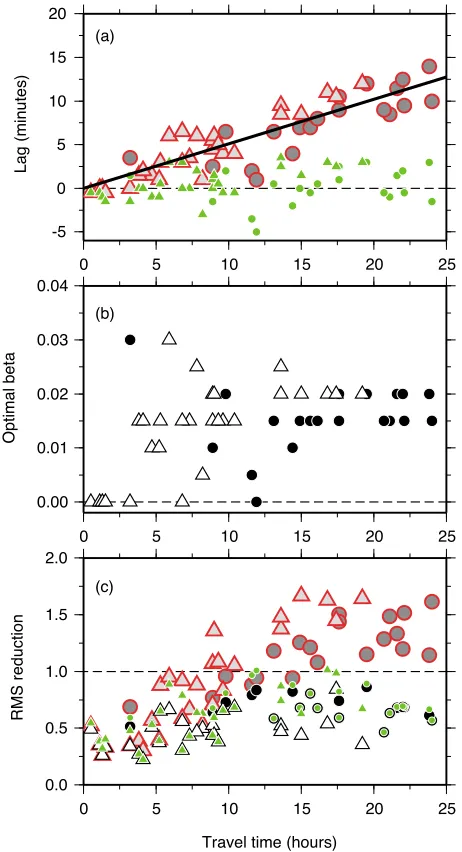
Fig. 5. (a) Lags with maximum correlation coefficients between the ob-servation and the simulation with (green)/without (red) the SAL effect, (b) optimal SAL factor (β) based on the maximum RMS reduction of the observation, and (c) RMS reduction of the observation by simulated results. These are shown as a function of the observed travel times at each OBP site. The linear fit in (a) shows a slope of 0.85%. Red and black indicate results without the SAL effect (β=0) and those with the optimalβat each OBP site, respectively. The results usingβ=0.015 is shown by green plots in (a) and (c). Triangles and circles indicate re-sults for the 2011 Tohoku and the 2010 Chilean tsunamis, respectively. The values for the plots are listed in Table 1.
Kuroshio current, by Isobe and Imawaki (2002) used pa-rameters ofh1 = 600 m,h2 =2400 m, andε =0.0020,
and give a deviation factor of 0.99984. Parameters found in other several two-layer models on western boundary cur-rents (Hurlburt, 1986; Yoon and Yasuda, 1987; Endoh and Hibiya, 2000) give a deviation factor 0.99981–0.99990, be-ing a 0.01–0.02% deviation from√g(h1+h2). Therefore,
the delay of the distant tsunami propagation behind√g H (0.8–1.0% deviation) arises mostly from the SAL effect, and weakly from ocean density stratification. Similar con-siderations have recently been conducted also by Watadaet al.(2012) and Tsaiet al.(2013).
As a consequence, the phase velocity of a giant tsunami is slower than√g H by∼1%.
We recommend that the loading effect is considered for simulating distant tsunami propagations with travel times in excess of several hours where discrepancies of simula-tion without loading effects result in tsunami arrivals of more than several minutes earlier than the observed tsunami (Fig. 5). Though a smallerβmay be preferred for tsunamis with smaller spatial scales, whose seismic magnitudes are probably smaller (M < 7–8), such smaller tsunamis be-come invisible in far fields. Also, changingβ barely de-teriorates simulated results, including tsunami waveforms, for near-field calculations (Figs. 4(e)–(f)). Thus, from the viewpoint of practical purposes, tsunami calculations using parameterization with the optimal value will also be use-ful for moderate tsunamis, as well as giant ones. Owing to an easy implementation and no increase in computational costs compared to standard long-wave calculations, the pro-posed method will immediately work for the early predic-tion/warning of future great tsunamis in both near and far fields (e.g., Weiet al., 2008; Tang et al., 2009; Tsushima et al., 2011), and possibly enable source inversions with Green’s functions including far-field data (e.g., Fujii and Satake, 2013).
The loading parameterization proposed in this study is the same method as used for classical ocean tide model-ing. As already noted by ocean tide modelers, convolu-tions of the whole global oceanic mass loading, rather than a simplified parameterization, are preferred to more pre-cisely calculate the loading deformation and its feedback (Ray, 1989; Matsumoto et al., 2000). Also, the interac-tion may be appropriately solved by a recent advanced sim-ulation scheme of Maeda and Furumura (2013) to collec-tively calculate seismic waves, ocean acoustic waves, and tsunamis. More powerful computer facilities than current supercomputer systems will be required to enable these pre-cise tsunami calculations.
Acknowledgments. The OBP data were downloaded from the websites of DART (http://www.ndbc.noaa.gov/dart.shtml) and JAMSTEC (http://www.jamstec.go.jp/scdc/top e.html). Numeri-cal simulations were carried out by the Altix 4700 supercomputer system of the National Institute for Earth Science and Disaster Prevention. We thank two reviewers for their valuable comments.
References
tidal potential alone, Phil. Trans. R. Soc. Lond. A, 290, 235–266, doi:10.1098/rsta.1978.0083, 1978.
Aida, I., Numerical experiments for the tsunami propagation—the 1964 Niigata tsunami and the 1968 Tokachi-oki tsunami,Bull. Earthq. Res. Inst.,47, 673–700, 1969.
Amante, C. and B. W. Eakins, ETOPO1 1 arc-minute global relief model: Procedures, data sources and analysis,NOAA Tech. Memo. NESDIS NGDC-24, 19 pp., 2009.
Comer, R. P., The tsunami mode of a flat earth and its excita-tion by earthquake sources,Geophys. J. R. Astron. Soc.,77, 1–27, doi:10.1111/j.1365-246X.1984.tb01923.x, 1984.
Endoh, T. and T. Hibiya, Numerical study of the generation and propaga-tion of trigger meanders of the Kuroshio south of Japan,J. Oceanogr., 56, 409–418, doi:10.1023/A:1011176322166, 2000.
Farrell, W. E., Deformation of the Earth by surface loads,Rev. Geophys. Space Phys.,10, 761–797, doi:10.1029/RG010i003p00761, 1972. Fujii, Y. and K. Satake, Slip distribution and seismic moment of the
2010 and 1960 Chilean earthquakes inferred from tsunami waveforms and coastal geodetic data, Pure Appl. Geophys., 170, 1493–1509, doi:10.1007/s00024-012-0524-2, 2013.
Gill, A. E., Adjustment under gravity of a density-stratified fluid, in
Atmosphere-Ocean Dynamics, p. 117–188, Academic Press, San Diego, 1982.
Gonz´alez, F. I., H. M. Milburn, E. N. Bernard, and J. Newman, Deep-ocean assessment and reporting of tsunamis (DART): Brief overview and status report,Proc. Int. Works. Tsunami Disaster Mitigation, 118– 129, 1998.
Grilli, S. T., J. C. Harris, T. S. T. Bakhsh, T. L. Masterlark, C. Kyriakopo-los, J. T. Kirby, and F. Shi, Numerical simulation of the 2011 Tohoku tsunami based on a new transient FEM co-seismic source: Comparison to far- and near-field observations,Pure Appl. Geophys.,170, 1333– 1359, doi:10.1007/s00024-012-0528-y, 2013.
Hirata, K., M. Aoyagi, H. Mikada, K. Kawaguchi, Y. Kaiho, R. Iwase, S. Morita, I. Fujisawa, H. Sugioka, K. Mitsuzawa, K. Sue-hiro, H. Kinoshita, and N. Fujiwara, Real-time geophysical mea-surements on the deep seafloor using submarine cable in the south-ern Kurile subduction zone, IEEE J. Oceanic Eng., 27, 170–181, doi:10.1109/JOE.2002.1002471, 2002.
Hurlburt, H. E., Dynamic transfer of simulated altimeter data into sub-surface information by a numerical ocean model,J. Geophys. Res.— Oceans,91, 2372–2400, doi:10.1029/JC091iC02p02372, 1986. Inazu, D., R. Hino, and H. Fujimoto, A global barotropic ocean model
driven by synoptic atmospheric disturbances for detecting seafloor ver-tical displacements from in situ ocean bottom pressure measurements,
Mar. Geophys. Res., 33, 127–148, doi:10.1007/s11001-012-9151-7, 2012.
Isobe, A. and S. Imawaki, Annual variation of the Kuroshio transport in a two-layer numerical model with a ridge,J. Phys. Oceanogr.,32, 994– 1009, doi:10.1175/1520-0485(2002)032<0994:AVOTKT>2.0.CO;2, 2002.
Jeffreys, H., Stress-differences in the Earth, inThe Earth: Its Origin, History and Physical Constitution, 6th ed., 263–285, Cambridge Univ. Press, New York, 1976.
Kajiura, K., The leading wave of a tsunami,Bull. Earthq. Res. Inst.,41, 535–571, 1963.
Kantha, L. H. and C. A. Clyason, Tides and tidal modeling, inNumerical Models of Oceans and Oceanic Processes, 375–492, Academic Press, San Diego, 2000.
Kato, T., Y. Terada, H. Nishimura, T. Nagai, and S. Koshimura, Tsunami records due to the 2010 Chile Earthquake observed by GPS buoys established along the Pacific coast of Japan,Earth Planets Space,63, e5–e8, doi:10.5047/eps.2011.05.001, 2011.
Kimura, T., S. Tanaka, and T. Saito, Ground tilt changes in Japan caused by the 2010 Maule, Chile, earthquake tsunami,J. Geophys. Res.—Solid Earth,118, 406–415, doi:10.1029/2012JB009657, 2013.
Kindle, J. C. and J. D. Thompson, The 26- and 50-day oscillations in the western Indian Ocean: Model results,J. Geophys. Res.—Oceans,94, 4721–4736, doi:10.1029/JC094iC04p04721, 1989.
Lamb, H., Surface waves, inHydrodynamics, 6th ed., p. 363–475, Dover, New York, 1932.
Maeda, T. and T. Furumura, FDM Simulation of seismic waves, ocean acoustic waves, and tsunamis based on tsunami-coupled equations of motion,Pure Appl. Geophys.,170, 109–127, doi:10.1007/s00024-011-0430-z, 2013.
Matsumoto, K., T. Takanezawa, and M. Ooe, Ocean tide models
devel-oped by assimilating TOPEX/POSEIDON altimeter data into hydro-logical model: A global model and a regional model around Japan,J. Oceanogr.,56, 567–581, doi:10.1023/A:1011157212596, 2000. Momma, H., N. Fujisawa, K. Kawaguchi, R. Iwase, S. Suzuki, and H.
Ki-noshita, Monitoring system for submarine earthquakes and deep sea en-vironment,Proc. Oceans 1997 Mar. Technol. Soc. IEEE Techno-Ocean 1997, 1453–1459, doi:10.1109/OCEANS.1997.624211, 1997. Parke, M. E., O1, P1, N2 models of the global ocean tide on an elastic earth
plus surface potential and spherical harmonic decompositions for M2, S2, and K1,Mar. Geod.,6, 35–81, doi:10.1080/15210608209379441, 1982.
Pierini, S., A Kuroshio Extension system model study: Decadal chaotic self-sustained oscillations,J. Phys. Oceanogr.,36, 1605–1625, doi:10.1175/JPO2931.1, 2006.
Qiu, B., Kuroshio Extension variability and forcing of the Pacific decadal oscillations: Responses and potential feedback,J. Phys. Oceanogr.,33, 2465–2482, doi:10.1175/2459.1, 2003.
Rabinovich, A. B., P. L. Woodworth, and V. V. Titov, Deep-sea observa-tions and modeling of the 2004 Sumatra tsunami in Drake Passage, Geo-phys. Res. Lett.,38, L16604, doi:10.1029/2011GL048305, 2011. Ray, R. D., Ocean self-attraction and loading in numerical tidal models,
Mar. Geod.,21, 181–192, doi:10.1080/01490419809388134, 1998. Saito, T., K. Satake, and T. Furumura, Tsunami waveform inversion
includ-ing dispersive waves: The 2004 earthquake off Kii Peninsula, Japan,J. Geophys. Res.—Solid Earth,115, B06303, doi:10.1029/2009JB006884, 2010.
Saito, T., Y. Ito, D. Inazu, and R. Hino, Tsunami source of the 2011 Tohoku-Oki earthquake, Japan: Inversion analysis based on dispersive tsunami simulations, Geophys. Res. Lett., 38, L00G19, doi:10.1029/2011GL049089, 2011.
Saito, T., D. Inazu, S. Tanaka, and T. Miyoshi, Tsunami coda across the Pa-cific Ocean following the 2011 Tohoku-Oki earthquake,Bull. Seismol. Soc. Am.,103, 1429–1443, doi:10.1785/0120120183, 2013.
Satake, K., The mechanism of the 1983 Japan Sea earthquake as inferred from long-period surface waves and tsunamis,Phys. Earth Planet. In-ter.,37, 249–260, doi:10.1016/0031-9201(85)90012-3, 1985. Stepanov, V. N. and C. W. Hughes, Parameterization of ocean
self-attraction and loading in numerical models of the ocean circulation,
J. Geophys. Res.—Oceans,109, C03037, doi:10.1029/2003JC002034, 2004.
Takahashi, R., On seismic sea waves caused by deformations of the sea bottom,Bull. Earthq. Res. Inst.,20, 375–400, 1942 (in Japanese with English abstract).
Tamisiea, M. E., E. M. Hill, R. M. Ponte, J. L. Davis, I. Velicogna, and N. T. Vinogradova, Impact of self-attraction and loading on the annual cycle in sea level,J. Geophys. Res.—Oceans, 115, C07004, doi:10.1029/2009JC005687, 2010.
Tang, L., V. V. Titov, and C. D. Chamberlin, Development, test-ing, and applications of site-specific tsunami inundation models for real-time forecasting, J. Geophys. Res.—Oceans, 114, C12025, doi:10.1029/2009JC005476, 2009.
Tang, L., V. V. Titov, E. N. Bernard, Y. Wei, C. D. Chamberlin, J. C. Newman, H. O. Mofjeld, D. Arcas, M. C. Eble, C. Moore, B. Uslu, C. Pells, M. Spillane, L. Wright, and E. Gica, Direct energy estimation of the 2011 Japan tsunami using deep-ocean pressure measurements,
J. Geophys. Res.—Oceans,117, C08008, doi:10.1029/2011JC007635, 2012.
Tsai, V. C., J.-P. Ampuero, H. Kanamori, and D. J. Stevenson, Estimating the effect of Earth elasticity and variable water density on tsunami speeds,Geophys. Res. Lett.,40, 492–496, doi:10.1002/grl.50147, 2013. Tsushima, H., K. Hirata, Y. Hayashi, Y. Tanioka, K. Kimura, S. Sakai, M. Shinohara, T. Kanazawa, R. Hino, and K. Maeda, Near-field tsunami forecasting using offshore tsunami data from the 2011 off the Pa-cific coast of Tohoku Earthquake,Earth Planets Space,63, 821–826, doi:10.5047/eps.2011.06.052, 2011.
Unoki, S., Waves and tides in a density-stratified ocean, in Physical Oceanography in Coastal Seas, 329–397, Tokai University Press, Tokyo, 1993 (in Japanese).
Ward, S. N., Relationships of tsunami generation and an earthquake source,J. Phys. Earth,28, 441–474, doi:10.4294/jpe1952.28.441, 1980. Watada, S., S. Kusumoto, Y. Fujii, and K. Satake, Cause of delayed first peak and reversed initial phase of distant tsunami, Abstract NH43B-1649,2012 AGU Fall Meeting, 2012.