Parsing with Soft and Hard Constraints on Dependency Length
∗Jason Eisner and Noah A. Smith
Department of Computer Science / Center for Language and Speech Processing Johns Hopkins University, Baltimore, MD 21218 USA
{jason,nasmith}@cs.jhu.edu
Abstract
In lexicalized phrase-structure or dependency parses, a word’s modifiers tend to fall near it in the string. We show that a crude way to use dependency length as a parsing feature can sub-stantially improve parsing speed and accuracy in English and Chinese, with more mixed results on German. We then show similar improvements by imposing hard bounds on dependency length and (additionally) modeling the resulting sequence of parse fragments. This simple “vine grammar” formalism has only finite-state power, but a context-free parameterization with some extra parameters for stringing fragments together. We ex-hibit a linear-time chart parsing algorithm with a low grammar constant.
1 Introduction
Many modern parsers identify the head word of each constituent they find. This makes it possible to identify the word-to-word dependencies implicit in a parse.1 (Some parsers, known as dependency parsers, even return these dependencies as their pri-mary output.)
Why bother to identify these dependencies? The typical reason is to model the fact that some word pairs are more likely than others to engage in a de-pendency relationship.2 In this paper, we propose a different reason to identify dependencies in candi-date parses: to evaluate not the dependency’s word pair but its length (i.e., the string distance between the two words). Dependency lengths differ from
∗
This work was supported by NSF ITR grant IIS-0313193 to the first author and a fellowship from the Fannie and John Hertz Foundation to the second author. The views expressed are not necessarily endorsed by the sponsors. The authors thank Mark Johnson, Eugene Charniak, Charles Schafer, Keith Hall, and John Hale for helpful discussion and Elliott Dr´abek and Markus Dreyer for insights on (respectively) Chinese and Ger-man parsing. They also thank an anonymous reviewer for sug-gesting the German experiments.
1In a phrase-structure parse, if phrase X headed by word
tokenxis a subconstituent of phraseY headed by word token
y 6= x, thenxis said to depend on y. In a more powerful compositional formalism like LTAG or CCG, dependencies can be extracted from the derivation tree.
2It has recently been questioned whether these “bilexical”
features actually contribute much to parsing performance (Klein and Manning, 2003; Bikel, 2004), at least when one has only a million words of training.
typical parsing features in that they cannot be deter-mined from tree-local information. Though lengths are not usually considered, we will see that bilexical dynamic-programming parsing algorithms can eas-ily consider them as they build the parse.
Soft constraints. Like any other feature of trees,
dependency lengths can be explicitly used as fea-tures in a probability model that chooses among trees. Such a model will tend to disfavor long de-pendencies (at least of some kinds), as these are em-pirically rare. In the first part of the paper, we show that such features improve a simple baseline depen-dency parser.
Hard constraints. If the bias against long
de-pendencies is strengthened into a hard constraint that absolutely prohibits long dependencies, then the parser turns into a partial parser with only finite-state power. In the second part of the paper, we show how to perform chart parsing in asymptotic linear time with a low grammar constant. Such a partial parser does less work than a full parser in practice, and in many cases recovers a more precise set of dependen-cies (with little loss in recall).
2 Short Dependencies in Langugage
We assume that correct parses exhibit a “short-dependency preference”: a word’s dependents tend to be close to it in the string.3 If thejthword of a sen-tence depends on theithword, then|i−j|tends to be
3
In this paper, we consider only a crude notion of “close-ness”: the number of intervening words. Other distance mea-sures could be substituted or added (following the literature on heavy-shift and sentence comprehension), including the phono-logical, morphophono-logical, syntactic, or referential (given/new) complexity of the intervening material (Gibson, 1998). In pars-ing, the most relevant previous work is due to Collins (1997), who considered three binary features of the intervening mate-rial: did it contain (a) any word tokens at all, (b) any verbs, (c) any commas or colons? Note that (b) is effective because it measures the length of a dependency in terms of the number of alternative attachment sites that the dependent skipped over, a notion that could be generalized. Similarly, McDonald et al. (2005) separately considered each of the intervening POS tags.
small. This implies that neitherinorjis modified by complex phrases that fall betweeniandj. In terms of phrase structure, it implies that the phrases mod-ifying word ifrom a given side tend to be (1) few in number, (2) ordered so that the longer phrases fall farther fromi, and (3) internally structured so that the bulk of each phrase falls on the side ofj away fromi.
These principles can be blamed for several lin-guistic phenomena. (1) helps explain the “late clo-sure” or “attach low” heuristic (e.g., Frazier, 1979; Hobbs and Bear, 1990): a modifier such as a PP is more likely to attach to the closest appropriate head. (2) helps account for heavy-shift: when an NP is long and complex, take NP out, put NP on the ta-ble, and give NP to Mary are likely to be rephrased as take out NP, put on the table NP, and give Mary NP. (3) explains certain non-canonical word orders: in English, a noun’s left modifier must become a right modifier if and only if it is right-heavy (a taller politician vs. a politician taller than all her rivals4), and a verb’s left modifier may extrapose its right-heavy portion (An aardvark walked in who had cir-cumnavigated the globe5).
Why should sentences prefer short dependencies? Such sentences may be easier for humans to produce and comprehend. Each word can quickly “discharge its responsibilities,” emitting or finding all its depen-dents soon after it is uttered or heard; then it can be dropped from working memory (Church, 1980; Gibson, 1998). Such sentences also succumb nicely to disambiguation heuristics that assume short de-pendencies, such as low attachment. Thus, to im-prove comprehensibility, a speaker can make stylis-tic choices that shorten dependencies (e.g., heavy-shift), and a language can categorically prohibit some structures that lead to long dependencies (*a taller-than-all-her-rivals politician; *the sentence
4
Whereas *a politician taller and *a
taller-than-all-her-rivals politician are not allowed. The phenomenon is pervasive.
5
This actually splits the heavy left dependent [an aardvark
who ...] into two non-adjacent pieces, moving the heavy second
piece. By slightly stretching the aardvark-who dependency in this way, it greatly shortens aardvark-walked. The same is pos-sible for heavy, non-final right dependents: I met an aardvark
yesterday who had circumnavigated the globe again stretches aardvark-who, which greatly shortens met-yesterday. These
ex-amples illustrate (3) and (2) respectively. However, the resulting non-contiguous constituents lead to non-projective parses that are beyond the scope of this paper.
that another sentence that had center-embedding was inside was incomprehensible).
Such functionalist pressures are not all-powerful. For example, many languages use SOV basic word order where SVO (or OVS) would give shorter de-pendencies. However, where the data exhibit some short-dependency preference, computer parsers as well as human parsers can obtain speed and accu-racy benefits by exploiting that fact.
3 Soft Constraints on Dependency Length
We now enhance simple baseline probabilistic parsers for English, Chinese, and German so that they consider dependency lengths. We confine our-selves (throughout the paper) to parsing part-of-speech (POS) tag sequences. This allows us to ig-nore data sparseness, out-of-vocabulary, smoothing, and pruning issues, but it means that our accuracy measures are not state-of-the-art. Our techniques could be straightforwardly adapted to (bi)lexicalized parsers on actual word sequences, though not neces-sarily with the same success.
3.1 Grammar Formalism
Throughout this paper we will use split bilexical grammars, or SBGs (Eisner, 2000), a notationally simpler variant of split head-automaton grammars, or SHAGs (Eisner and Satta, 1999). The formalism is context-free. We define here a probabilistic ver-sion,6 which we use for the baseline models in our experiments. They are only baselines because the SBG generative process does not take note of de-pendency length.
An SBG is an tuple G = (Σ,$, L, R). Σ is an alphabet of words. (In our experiments, we parse only POS tag sequences, soΣis actually an alpha-bet of tags.) $ 6∈ Σis a distinguished root symbol;
let Σ = Σ¯ ∪ {$}. L and R are functions from Σ¯
to probabilistic -free finite-state automata overΣ. Thus, for eachw ∈Σ, the SBG specifies “left” and¯ “right” probabilistic FSAs,LwandRw.
We useLw(G) : ¯Σ∗ → [0,1]to denote the
prob-abilistic context-free language of phrases headed by
w. Lw(G) is defined by the following simple
top-down stochastic process for sampling from it:
6There is a straightforward generalization to weighted
1. Sample from the finite-state language L(Lw) a
sequence λ = w−1w−2. . . w−` ∈ Σ∗ of left
children, and from L(Rw) a sequence ρ =
w1w2. . . wr ∈ Σ∗ of right children. Each
se-quence is found by a random walk on its proba-bilistic FSA. We say the children depend onw.
2. For eachifrom −`to r withi 6= 0, recursively sample αi ∈ Σ∗ from the context-free language
Lwi(G). It is this step that indirectly determines
dependency lengths.
3. Return α−`. . . α−2α−1wα1α2. . . αr ∈ Σ¯∗, a
concatenation of strings.
Notice thatw’s left childrenλwere generated in reverse order, sow−1andw1are its closest children whilew−`andwrare the farthest.
Given an input sentenceω =w1w2. . . wn ∈Σ∗,
a parser attempts to recover the highest-probability derivation by which $ω could have been generated
fromL$(G). Thus, $ plays the role ofw0. A sample
derivation is shown in Fig. 1a. Typically, L$ and R$ are defined so that $ must have no left children
(` = 0) and at most one right child (r ≤ 1), the latter serving as the conventional root of the parse.
3.2 Baseline Models
In the experiments reported here, we defined only
very simple automata for Lw and Rw (w ∈ Σ).
However, we tried three automaton types, of vary-ing quality, so as to evaluate the benefit of addvary-ing length-sensitivity at three different levels of baseline performance.
In model A (the worst), each automaton has topol-ogy }, with a single state q1, so token w’s left
dependents are conditionally independent of one an-other given w. In model C (the best), each au-tomaton }−→}has an extra state q0 that al-lows the first (closest) dependent to be chosen dif-ferently from the rest. Model B is a compromise:7
it is like model A, but each type w ∈ Σ may
have an elevated or reduced probability of having no dependents at all. This is accomplished by
us-ing automata }−→}as in model C, which
al-lows the stopping probabilities p(STOP | q0) and
p(STOP |q1)to differ, but tying the conditional
dis-7It is equivalent to the “dependency model with valence” of
Klein and Manning (2004).
tributionsp(q0−→w q1 | q0,¬STOP)andp(q1−→w q1 |
q1,¬STOP).
Finally, in§3,L$ andR$ are restricted as above,
soR$ gives a probability distribution overΣonly.
3.3 Length-Sensitive Models
None of the baseline models A–C explicitly model the distance between a head and child. We enhanced them by multiplying in some extra length-sensitive factors when computing a tree’s probability. For each dependency, an extra factorp(∆| . . .)is mul-tiplied in for the probability of the dependency’s length∆ = |i−j|, whereiandjare the positions of the head and child in the surface string.8
Again we tried three variants. In one version, this new probabilityp(∆|. . .)is conditioned only on the direction d = sign(i−j) of the dependency. In another version, it is conditioned only on the POS taghof the head. In a third version, it is conditioned ond,h, and the POS tagcof the child.
3.4 Parsing Algorithm
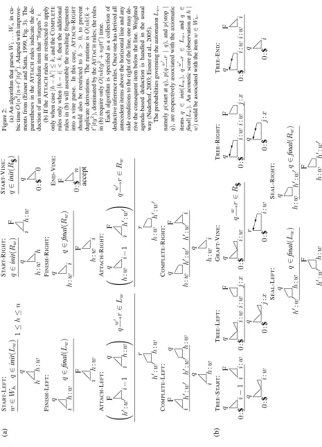
Fig. 2a gives a variant of Eisner and Satta’s (1999) SHAG parsing algorithm, adapted to SBGs, which are easier to understand.9 (We will modify this al-gorithm later in§4.) The algorithm obtainsO(n3) runtime, despite the need to track the position of head words, by exploiting the conditional indepen-dence between a head’s left children and right chil-dren. It builds “half-constituents” denoted by @@
(a head word together with some modifying phrases on the right, i.e.,wα1. . . αr) and (a head word
together with some modifying phrases on the left, i.e., α−`. . . α−1w). A new dependency is
intro-duced when @@ + are combined to get
H H
or
(a pair of linked head words with all the intervening phrases, i.e.,wα1. . . αrα0−`0. . . α0−1w0,
where wis respectively the parent or child of w0).
One can then combine HH
+ @@ = @@ , or
8Since the∆values are fully determined by the tree but
ev-eryp(∆ | . . .) ≤1, this crude procedure simply reduces the probability mass of every legal tree. The resulting model is
de-ficient (does not sum to 1); the remaining probability mass goes
to impossible trees whose putative dependency lengths∆are inconsistent with the tree structure. We intend in future work to explore non-deficient models (log-linear or generative), but even the present crude approach helps.
9The SHAG notation was designed to highlight the
+
= . Only O(n3) combinations
are possible in total when parsing a length-n sen-tence.
3.5 A Note on Word Senses
[This section may be skipped by the casual reader.] A remark is necessary about :wand :w0in Fig. 2a, which represent senses of the words at positions
h and h0. Like past algorithms for SBGs (Eisner, 2000), Fig. 2a is designed to be a bit more general and integrate sense disambiguation into parsing. It formally runs on an input Ω = W1. . . Wn ⊆ Σ∗,
where eachWi ⊆ Σis a “confusion set” over
pos-sible values of the ith word w
i. The algorithm
re-covers the highest-probability derivation that gener-ates $ω for someω ∈ Ω(i.e.,ω = w1. . . wn with
(∀i)wi ∈Wi).
This extra level of generality is not needed for any of our experiments, but it is needed for SBG parsers to be as flexible as SHAG parsers. We include it in this paper to broaden the applicability of both Fig. 2a and our extension of it in§4.
The “senses” can be used in an SBG to pass a finite amount of information between the left and right children of a word, just as SHAGs allow.10 For example, to model the fronting of a direct object, an SBG might use a special sense of a verb, whose au-tomata tend to generate both one more noun inλand one fewer noun inρ.
Senses can also be used to pass information
be-tween parents and children. Important uses are
to encode lexical senses, or to enrich the de-pendency parse with constituent labels or
depen-10Fig. 2a enhances the Eisner-Satta version with explicit
senses while matching its asymptotic performance. On this point, see (Eisner and Satta, 1999,§8 and footnote 6). How-ever, it does have a practical slowdown, in that START-LEFT
nondeterministically guesses every possible sense ofWi, and these senses are pursued separately. To match the Eisner-Satta algorithm, we should not need to commit to a word’s sense un-til we have seen all its left children. That is, left triangles and left trapezoids should not carry a sense :wat all, except for the completed left triangle (marked F) that is produced by FINISH -LEFT. FINISH-LEFTshould choose a sensewofWh accord-ing to the final stateq, which reflects knowledge ofWh’s left children. For this strategy to work, the transitions inLw(used by ATTACH-LEFT) must not depend on the particular sensew
but only onW. In other words, allLw : w ∈ Whare really copies of a sharedLWh, except that they may have different fi-nal states. This requirement involves no loss of generality, since the nondeterministic sharedLWhis free to branch as soon as it likes onto paths that commit to the various sensesw.
dency labels (Eisner, 2000). For example, the in-put token Wi = {bank1/N/NP, bank2/N/NP,
bank3/V /VP, bank3/V /S} ⊂ Σ allows four
“senses” of bank, namely two nominal meanings, and two syntactically different versions of the verbal meaning, whose automata require them to expand into VP and S phrases respectively.
The cubic runtime is proportional to the num-ber of ways of instantiating the inference rules in Fig. 2a: O(n2(n+t0)tg2), where n = |Ω| is the input length, g = maxni=1|Wi|bounds the size of
a confusion set, tbounds the number of states per automaton, and t0 ≤ t bounds the number of au-tomaton transitions from a state that emit the same word. For deterministic automata,t0= 1.11
3.6 Probabilistic Parsing
It is easy to make the algorithm of Fig. 2a length-sensitive. When a new dependency is added by an ATTACH rule that combines @@ + , the
an-notations on @@ and suffice to determine
the dependency’s length ∆ = |h −h0|, direction
d = sign(h− h0), head word w, and child word
w0.12 So the additional cost of such a dependency,
e.g. p(∆ | d, w, w0), can be included as the weight
of an extra antecedent to the rule, and so included in the weight of the resulting or HH .
To execute the inference rules in Fig. 2a, we use a prioritized agenda. Derived items such as
@
@ , , , and HH are prioritized by
their Viterbi-inside probabilities. This is known as uniform-cost search or shortest-hyperpath search (Nederhof, 2003). We halt as soon as a full parse (the accept item) pops from the agenda, since uniform-cost search (as a special case of the A∗ algorithm) guarantees this to be the maximum-probability parse. No other pruning is done.
11
Confusion-set parsing may be regarded as parsing a par-ticular lattice withn states andng arcs. The algorithm can be generalized to lattice parsing, in which case it has runtime
O(m2(n+t0
)t)for a lattice ofnstates andmarcs. Roughly,
h:wis replaced by an arc, whileiis replaced by a state and
i−1is replaced by the same state.
12
For general lattice parsing, it is not possible to determine∆
With a prioritized agenda, a probability model that more sharply discriminates among parses will typically lead to a faster parser. (Low-probability constituents languish at the back of the agenda and are never pursued.) We will see that the length-sensitive models do run faster for this reason.
3.7 Experiments with Soft Constraints
We trained models A–C, using unsmoothed maxi-mum likelihood estimation, on three treebanks: the Penn (English) Treebank (split in the standard way, §2–21 train/§23 test, or 950K/57K words), the Penn Chinese Treebank (80% train/10% test or 508K/55K words), and the German TIGER corpus (80%/10%
or 539K/68K words).13 Estimation was a simple
matter of counting automaton events and normaliz-ing counts into probabilities. For each model, we also trained the three length-sensitive versions de-scribed in§3.3.
The German corpus contains non-projective trees. None of our parsers can recover non-projective de-pendencies (nor can our models produce them). This fact was ignored when counting events for maxi-mum likelihood estimation: in particular, we always trainedLwandRwon the sequence ofw’s
immedi-ate children, even in non-projective trees.
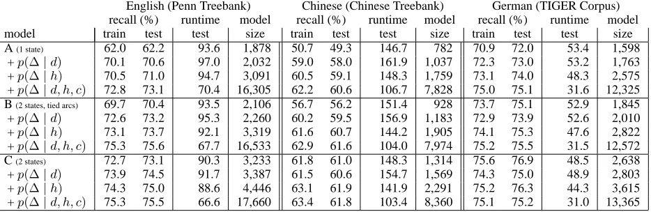
Our results (Tab. 1) show that sharpening the probabilities with the most sophisticated distance factors p(∆ | d, h, c), consistently improved the speed of all parsers.14 The change to the code is trivial. The only overhead is the cost of looking up and multiplying in the extra distance factors.
Accuracy also improved over the baseline mod-els of English and Chinese, as well as the simpler baseline models of German. Again, the most so-phisticated distance factors helped most, but even the simplest distance factor usually obtained most of the accuracy benefit.
German model C fell slightly in accuracy. The speedup here suggests that the probabilities were sharpened, but often in favor of the wrong parses. We did not analyze the errors on German; it may
13Heads were extracted for English using Michael Collins’
rules and Chinese using Fei Xia’s rules (defaulting in both cases to right-most heads where the rules fail). German heads were extracted using the TIGER Java API; we discarded all resulting dependency structures that were cyclic or unconnected (6%).
14We measure speed abstractly by the number of items built
and pushed on the agenda.
be relevant that 25% of the German sentences con-tained a projective dependency between non-punctuation tokens.
Studying the parser output for English, we found that the length-sensitive models preferred closer at-tachments, with 19.7% of tags having a nearer parent in the best parse under model C withp(∆ |d, h, c) than in the original model C, 77.7% having a par-ent at the same distance, and only 2.5% having a farther parent. The surviving long dependencies (at any length>1) tended to be much more accurate, while the (now more numerous) length-1 dependen-cies were slightly less accurate than before.
We caution that length sensitivity’s most dramatic improvements to accuracy were on the worse base-line models, which had more room to improve. The better baseline models (B and C) were already able to indirectly capture some preference for short de-pendencies, by learning that some parts of speech were unlikely to have multiple left or multiple right
dependents. Enhancing B and C therefore
con-tributed less, and indeed may have had some harmful effect by over-penalizing some structures that were already appropriately penalized.15 It remains to be seen, therefore, whether distance features would help state-of-the art parsers that are already much better than model C. Such parsers may already in-corporate features that indirectly impose a good model of distance, though perhaps not as cheaply.
4 Hard Dependency-Length Constraints
We have seen how an explicit model of distance can improve the speed and accuracy of a simple proba-bilistic dependency parser. Another way to capital-ize on the fact that most dependencies are local is to impose a hard constraint that simply forbids long dependencies.
The dependency trees that satisfy this constraint yield a regular string language.16The constraint pre-vents arbitrarily deep center-embedding, as well as arbitrarily many direct dependents on a given head,
15Owing to our deficient model. A log-linear or
discrimina-tive model would be trained to correct for overlapping penalties and would avoid this risk. Non-deficient generative models are also possible to design, along lines similar to footnote 16.
16One proof is to construct a strongly equivalent CFG without
center-embedding (Nederhof, 2000). Each nonterminal has the formhw, q, i, ji, wherew∈Σ,qis a state ofLworRw, and
English (Penn Treebank) Chinese (Chinese Treebank) German (TIGER Corpus) recall (%) runtime model recall (%) runtime model recall (%) runtime model model train test test size train test test size train test test size A(1 state) 62.0 62.2 93.6 1,878 50.7 49.3 146.7 782 70.9 72.0 53.4 1,598
+p(∆|d) 70.1 70.6 97.0 2,032 59.0 58.0 161.9 1,037 72.3 73.0 53.2 1,763 +p(∆|h) 70.5 71.0 94.7 3,091 60.5 59.1 148.3 1,759 73.1 74.0 48.3 2,575 +p(∆|d, h, c) 72.8 73.1 70.4 16,305 62.2 60.6 106.7 7,828 75.0 75.1 31.6 12,325 B(2 states, tied arcs) 69.7 70.4 93.5 2,106 56.7 56.2 151.4 928 73.7 75.1 52.9 1,845
+p(∆|d) 72.6 73.2 95.3 2,260 60.2 59.5 156.9 1,183 72.9 73.9 52.6 2,010 +p(∆|h) 73.1 73.7 92.1 3,319 61.6 60.7 144.2 1,905 74.1 75.3 47.6 2,822 +p(∆|d, h, c) 75.3 75.6 67.7 16,533 62.9 61.6 104.0 7,974 75.2 75.5 31.5 12,572 C(2 states) 72.7 73.1 90.3 3,233 61.8 61.0 148.3 1,314 75.6 76.9 48.5 2,638
+p(∆|d) 73.9 74.5 91.7 3,387 61.5 60.6 154.7 1,569 74.3 75.0 48.9 2,803 +p(∆|h) 74.3 75.0 88.6 4,446 63.1 61.9 141.9 2,291 75.2 76.3 44.3 3,615 +p(∆|d, h, c) 75.3 75.5 66.6 17,660 63.4 61.8 103.4 8,360 75.1 75.2 31.0 13,365
Table 1: Dependency parsing of POS tag sequences with simple probabilistic split bilexical grammars. The models differ only in how they weight the same candidate parse trees. Length-sensitive models are larger but can improve dependency accuracy and speed. (Recall is measured as the fraction of non-punctuation tags whose correct parent (if not the $ symbol) was correctly recovered by the parser; it equals precision, unless the parser left some sentences unparsed (or incompletely parsed, as in§4), in
which case precision is higher. Runtime is measured abstractly as the average number of items (i.e., @@ , , , HH )
built per word. Model size is measured as the number of nonzero parameters.)
either of which would allow the non-regular lan-guage {anbcn : 0 < n < ∞}. It does allow
ar-bitrarily deep right- or left-branching structures.
4.1 Vine Grammars
The tighter the bound on dependency length, the fewer parse trees we allow and the faster we can find them using the algorithm of Fig. 2a. If the bound is too tight to allow the correct parse of some sen-tence, we would still like to allow an accurate partial parse: a sequence of accurate parse fragments (Hin-dle, 1990; Abney, 1991; Appelt et al., 1993; Chen, 1995; Grefenstette, 1996). Furthermore, we would like to use the fact that some fragment sequences are presumably more likely than others.
Our partial parses will look like the one in Fig. 1b. where 4 subtrees rather than 1 are dependent on $. This is easy to arrange in the SBG formalism. We merely need to construct our SBG so that the au-tomaton R$ is now permitted to generate multiple
children—the roots of parse fragments.
This R$ is a probabilistic finite-state automaton
that describes legal or likely root sequences inΣ∗. In our experiments in this section, we will train it to be a first-order (bigram) Markov model. (Thus we constructR$ in the usual way to have |Σ|+ 1 states, and train it on data like the other left and right automata. During generation, its state remembers the previously generated root, if any. Recall that we are working with POS tag sequences, so the roots,
like all other words, are tags inΣ.)
The 4 subtrees in Fig. 1b appear as so many bunches of grapes hanging off a vine. We refer to the dotted dependencies upon $ as vine dependen-cies, and the remaining, bilexical dependencies as tree dependencies.
One might informally use the term “vine gram-mar” (VG) for any generative formalism, intended for partial parsing, in which a parse is a constrained sequence of trees that cover the sentence. In gen-eral, a VG might use a two-part generative process: first generate a finite-state sequence of roots, then expand the roots according to some more powerful formalism. Conveniently, however, SBGs and other dependency grammars can integrate these two steps into a single formalism.
4.2 Feasible Parsing
(a) $ would
```````````````````````````````````````aaaaaaaaaaaaaaaaaaaaeeeeeYYYYY
[
\ the rule filings
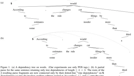
eeeee byYYYYY . Figure 1: (a) A dependency tree on words. (Our experiments use only POS tags.) (b) A partial
parse for the same sentence retaining only tree dependencies of length≤k = 3. The roots of the 4 resulting parse fragments are now connected only by their dotted-line “vine dependencies” on $. Transforming (a) into (b) involves grafting subtrees rooted at “According”, “,”, and “.” onto the vine.
are also the traditional way to describe finite-state sublanguages within a context-free grammar. By contrast, our limitation on dependency length en-sures regularity while still allowing (for any bound
k ≥ 1) arbitrarily wide and deep trees, such as
a→b→. . .→ root←. . .←y←z.
Our goal is to find the best feasible parse (if any). Rather than transform the grammar as in foot-note 16, our strategy is to modify the parser so that it only considers feasible parses. The interesting prob-lem is to achieve linear-time parsing with a grammar constant that is as small as for ordinary parsing.
We also correspondingly modify the training data so that we only train on feasible parses. That is, we break any long dependencies and thereby fragment each training parse (a single tree) into a vine of one or more restricted trees. When we break a child-to-parent dependency, we reattach the child to $.17 This process, grafting, is illustrated in Fig. 1. Al-though this new parse may score less than 100% re-call of the original dependencies, it is the best feasi-ble parse, so we would like to train the parser to find it.18 By training on the modified data, we learn more
17Any dependency covering the child must also be broken to
preserve projectivity. This case arises later; see footnote 25.
18Although the parser will still not be able to find it if it is
non-projective (possible in German). Arguably we should have defined “feasible” to also require projectivity, but we did not.
appropriate statistics for bothR$ and the other
au-tomata. If we trained on the original trees, we would inaptly learn thatR$ always generates a single root
rather than a certain kind of sequence of roots. For evaluation, we score tree dependencies in our feasible parses against the tree dependencies in the unmodified gold standard parses, which are not nec-essarily feasible. We also show oracle performance.
4.3 Approach #1: FSA Parsing
Since we are now dealing with a regular language, it is possible in principle to use a weighted finite-state automaton (FSA) to search for the best feasible parse. The idea is to find the highest-weighted path that accepts the input stringω = w1w2. . . wn.
Us-ing the Viterbi algorithm, this takes timeO(n). The trouble is that this linear runtime hides a con-stant factor, which depends on the size of the rele-vant part of the FSA and may be enormous for any correct FSA.19
Consider an example from Fig 1b.
Af-ter nondeAf-terministically reading w1. . . w11 = According. . . insider along the correct path, the FSA state must record (at least) that insider has no parent yet and thatR$ andRcutare in particular states that
19
may still accept more children. Else the FSA cannot know whether to accept a continuationw12. . . wn.
In general, after parsing a prefix w1. . . wj, the
FSA state must somehow record information about all incompletely linked words in the past. It must record the sequence of past words wi (i ≤ j) that
still need a parent or child in the future; ifwi still
needs a child, it must also record the state ofRwi.
Our restriction to dependency length≤kis what allows us to build a finite-state machine (as opposed to some kind of pushdown automaton with an un-bounded number of configurations). We need only build the finitely many states where the incompletely linked words are limited to at mostw0=$ and thek most recent words,wj−k+1. . . wj. Other states
can-not extend into a feasible parse, and can be pruned. However, this still allows the FSA to be in
O(2ktk+1) different states after reading w1. . . wj.
Then the runtime of the Viterbi algorithm, though linear inn, is exponential ink.
4.4 Approach #2: Ordinary Chart Parsing
A much better idea for most purposes is to use a chart parser. This allows the usual dynamic pro-gramming techniques for reusing computation. (The FSA in the previous section failed to exploit many such opportunities: exponentially many states would have proceeded redundantly by building the same
wj+1wj+2wj+3constituent.)
It is simple to restrict our algorithm of Fig. 2a to find only feasible parses. It is the ATTACH rules
@
@ + that add dependencies: simply use a
side condition to block them from applying unless |h−h0| ≤k(short tree dependency) orh= 0(vine
dependency). This ensures that all HH
and
will have width≤kor have their left edge at 0. One might now incorrectly expect runtime linear inn: the number of possible ATTACHcombinations is reduced fromO(n3)toO(nk2), becauseiandh0
are now restricted to a narrow range givenh.
Unfortunately, the half-constituents @@ and
may still be arbitrarily wide, thanks to arbi-trary right- and left-branching: a feasible vine parse may be a sequence of wide trees @@ . Thus there
areO(n2k)possible COMPLETEcombinations, not to mention O(n2) ATTACH-RIGHT combinations for whichh= 0. So the runtime remains quadratic.
4.5 Approach #3: Specialized Chart Parsing
How, then, do we get linear runtime and a rea-sonable grammar constant? We give two ways to achieve runtime ofO(nk2).
First, we observe without details that we can eas-ily achieve this by starting instead with the algo-rithm of Eisner (2000),20 rather than Eisner and Satta (1999), and again refusing to add long tree de-pendencies. That algorithm effectively concatenates only trapezoids, not triangles. Each is spanned by a single dependency and so has width≤k. The vine dependencies do lead to wide trapezoids, but these are constrained to start at 0, where $ is. So the algo-rithm tries at mostO(nk2)combinations of the form
h i+i j(like the ATTACHcombinations above)
andO(nk)combinations of the form0 i+i j,
wherei−h≤k, j−i≤k. The precise runtime is
O(nk(k+t0)tg3).
We now propose a hybrid linear-time algorithm that further improves runtime toO(nk(k+t0)tg2), saving a factor ofg in the grammar constant.21 We observe that since within-tree dependencies must have length ≤ k, they can all be captured within Eisner-Satta trapezoids of width≤ k. So our VG
parse @@
∗can be assembled by simply
concate-nating a sequence( ∗ HH ∗
@
@ )∗of these
narrow trapezoids interspersed with width-0 trian-gles. As this is a regular sequence, we can assem-ble it in linear time from left to right (rather than in the order of Eisner and Satta (1999)), multiplying the items’ probabilities together. Whenever we start adding the right half HH ∗
@
@ of a tree along the
vine, we have discovered that tree’s root, so we mul-tiply in the probability of a $←root dependency.
Formally, our hybrid parsing algorithm restricts the original rules of Fig. 2a to build only trapezoids of width ≤ k and triangles of width < k.22 The additional inference rules in Fig. 2b then assemble the final VG parse as just described.
20
With a small change that when two items are combined, the
right item (rather than the left) must be simple.
21This savings comes from building the internal structure of
a trapezoid from both ends inward rather than from left to right. The corresponding unrestricted algorithms (Eisner, 2000; Eis-ner and Satta, 1999, respectively) have exactly the same run-times withkreplaced byn.
22For the experiments of§4.7, wherekvaried by type, we
0.4 0.5 0.6 0.7 0.8 0.9 1
0.3 0.4 0.5 0.6 0.7 0.8 0.9 recall
precision
E
C
G
k = 1
Model C, no bound single bound (English) (Chinese) (German)
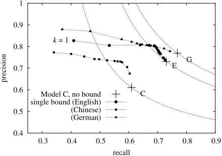
Figure 3: Trading precision and recall: Imposing bounds can improve precision at the expense of recall, for English and Chi-nese. German performance suffers more. Bounds shown are
k ={1,2, ...,10,15,20}. The dotted lines show constantF -measure of the unbounded model.
4.6 Experiments with Hard Constraints
Our experiments used the asymptotically fast hybrid parsing algorithm above. We used the same left and right automata as in model C, the best-performing model from §3.2. However, we now define R$ to
be a first-order (bigram) Markov model (§4.1). We trained and tested on the same headed treebanks as before (§3.7), except that we modified the training trees to make them feasible (§4.2).
Results are shown in Figures 3 (precision/recall tradeoff) and 4 (accuracy/speed tradeoff), for k ∈ {1,2, ...,10,15,20}. Dots correspond to different values ofk. On English and Chinese, some values of
k actually achieve betterF-measure accuracy than the unbounded parser, by eliminating errors.23
We observed that changing R$ from a bigram
to a unigram model significantly hurt performance, showing that it is in fact useful to empirically model likely sequences of parse fragments.
4.7 Finer-Grained Hard Constraints
The dependency length boundkneed not be a sin-gle value. Substantially better accuracy can be re-tained if each dependency type—each (h, c, d) = (head tag, child tag, direction) tuple—has its own
23
Because our prototype implementation of each kind of parser (baseline, soft constraints, single-bound, and type-specific bounds) is known to suffer from different inefficiencies, runtimes in milliseconds are not comparable across parsers. To give a general idea, 60-word English sentences parsed in around 300ms with no bounds, but at around 200ms with either a dis-tance modelp(∆|d, h, c)or a generous hard bound ofk= 10.
boundk(h, c, d). We call these type-specific bounds: they create a many-dimensional space of possible parsers. We measured speed and accuracy along a sensible path through this space, gradually tighten-ing the bounds ustighten-ing the followtighten-ing process:
1. Initialize each bound k(h, c, d) to the maximum distance observed in training (or 1 for unseen triples).24
2. Greedily choose a bound k(h, c, d) such that, if its value is decremented and trees that violate the new bound are accordingly broken, the fewest de-pendencies will be broken.25
3. Decrement the bound k(h, c, d) and modify the training data to respect the bound by breaking de-pendencies that violate the bound and “grafting” the loose portion onto the vine. Retrain the parser on the training data.
4. If all bounds are not equal to 1, go to step 2. The performance of every 200thmodel along the trajectory of this search is plotted in Fig. 4.26 The graph shows that type-specific bounds can speed up the parser to a given level with less loss in accuracy.
5 Related Work
As discussed in footnote 3, Collins (1997) and Mc-Donald et al. (2005) considered the POS tags inter-vening between a head and child. These soft con-straints were very helpful, perhaps in part because they helped capture the short dependency preference (§2). Collins used them as conditioning variables and McDonald et al. as log-linear features, whereas our§3 predicted them directly in a deficient model.
As for hard constraints (§4), our limitation on de-pendency length can be regarded as approximating a context-free language by a subset that is a regular
24
In the case of the German TIGER corpus, which contains non-projective dependencies, we first make the training trees into projective vines by raising all non-projective child nodes to become heads on the vine.
25
Not counting dependencies that must be broken indirectly in order to maintain projectivity. (If word 4 depends on word 7 which depends on word 2, and the 4 → 7 dependency is broken, making 4 a root, then we must also break the2→ 7
dependency.)
26Note thatk(h, c,right) = 7bounds the width of
@
@ +
=
. For a finer-grained approach, we could
in-stead separately bound the widths of @@ and , say by
language. Our “vines” then let us concatenate sev-eral strings in this subset, which typically yields a superset of the original context-free language. Sub-set and superSub-set approximations of (weighted) CFLs by (weighted) regular languages, usually by pre-venting center-embedding, have been widely ex-plored; Nederhof (2000) gives a thorough review. We limit all dependency lengths (not just center-embedding).27 Further, we derive weights from a modified treebank rather than by approximating the true weights. And though regular grammar approxi-mations are useful for other purposes, we argue that for parsing it is more efficient to perform the approx-imation in the parser, not in the grammar.
Brants (1999) described a parser that encoded the grammar as a set of cascaded Markov models. The decoder was applied iteratively, with each iteration transforming the best (or n-best) output from the previous one until only the root symbol remained. This is a greedy variant of CFG parsing where the grammar is in Backus-Naur form.
Bertsch and Nederhof (1999) gave a linear-time recognition algorithm for the recognition of the reg-ular closure of deterministic context-free languages. Our result is related; instead of a closure of deter-ministic CFLs, we deal in a closure of CFLs that are assumed (by the parser) to obey some constraint on trees (like a maximum dependency length).
6 Future Work
The simple POS-sequence models we used as an ex-perimental baseline are certainly not among the best parsers available today. They were chosen to illus-trate how modeling and exploiting distance in syntax can affect various performance measures. Our ap-proach may be helpful for other kinds of parsers as well. First, we hope that our results will generalize to more expressive grammar formalisms such as lex-icalized CFG, CCG, and TAG, and to more expres-sively weighted grammars, such as log-linear mod-els that can include head-child distance among other rich features. The parsing algorithms we presented also admit inside-outside variants, allowing iterative estimation methods for log-linear models (see, e.g., Miyao and Tsujii, 2002).
27Of course, this still allows right-branching or
left-branching to unbounded depth.
0.5
Figure 4: Trading off speed and accuracy by varying the set of feasible parses: The baseline (no length bound) is shown as+. Tighter bounds always improve speed, except for the most lax bounds, for which vine construction overhead incurs a slowdown. Type-specific bounds tend to maintain goodF -measure at higher speeds than the single-bound approach. The vertical error bars show the “oracle” accuracy for each experi-ment (i.e., theF-measure if we had recovered the best feasible parse, as constructed from the gold-standard parse by grafting: see§4.2). Runtime is measured as the number of items per word
Second, fast approximate parsing may play a role in more accurate parsing. It might be used to rapidly compute approximate outside-probability estimates to prioritize best-first search (e.g., Caraballo and Charniak, 1998). It might also be used to speed up the early iterations of training a weighted parsing model, which for modern training methods tends to require repeated parsing (either for the best parse, as by Taskar et al., 2004, or all parses, as by Miyao and Tsujii, 2002).
Third, it would be useful to investigate algorith-mic techniques and empirical benefits for limiting dependency length in more powerful grammar for-malisms. Our runtime reduction from O(n3) →
O(nk2) for a length-k bound applies only to a “split” bilexical grammar.28 Various kinds of syn-chronous grammars, in particular, are becoming im-portant in statistical machine translation. Their high runtime complexity might be reduced by limiting monolingual dependency length (for a related idea see Schafer and Yarowsky, 2003).
Finally, consider the possibility of limiting depen-dency length during grammar induction. We reason that a learner might start with simple structures that focus on local relationships, and gradually relax this restriction to allow more complex models.
7 Conclusion
We have described a novel reason for identifying headword-to-headword dependencies while parsing:
to consider their length. We have demonstrated
that simple bilexical parsers of English, Chinese, and German can exploit a “short-dependency pref-erence.” Notably, soft constraints on dependency length can improve both speed and accuracy, and hard constraints allow improved precision and speed with some loss in recall (on English and Chinese, remarkably little loss). Further, for the hard con-straint “length≤k,” we have given anO(nk2) par-tial parsing algorithm for split bilexical grammars; the grammar constant is no worse than for state-of-the-artO(n3)algorithms. This algorithm strings to-gether the partial trees’ roots along a “vine.”
28
The obvious reduction for unsplit head automaton gram-mars, say, is onlyO(n4) → O(n3k), following (Eisner and
Satta, 1999). Alternatively, one can convert the unsplit HAG to a split one that preserves the set of feasible (length≤k) parses, but thengbecomes prohibitively large in the worst case.
Our approach might be adapted to richer parsing formalisms, including synchronous ones, and should be helpful as an approximation to full parsing when fast, high-precision recovery of syntactic informa-tion is needed.
References
S. P. Abney. Parsing by chunks. In Principle-Based Parsing:
Computation and Psycholinguistics. Kluwer, 1991.
D. E. Appelt, J. R. Hobbs, J. Bear, D. Israel, and M. Tyson. FASTUS: A finite-state processor for information extraction from real-world text. In Proc. of IJCAI, 1993.
E. Bertsch and M.-J. Nederhof. Regular closure of deterministic languages. SIAM J. on Computing, 29(1):81–102, 1999. D. Bikel. A distributional analysis of a lexicalized statistical
parsing model. In Proc. of EMNLP, 2004.
T. Brants. Cascaded Markov models. In Proc. of EACL, 1999. S. A. Caraballo and E. Charniak. New figures of merit for
best-first probabilistic chart parsing. Computational Linguistics, 24(2):275–98, 1998.
S. Chen. Bayesian grammar induction for language modeling. In Proc. of ACL, 1995.
K. W. Church. On memory limitations in natural language pro-cessing. Master’s thesis, MIT, 1980.
M. Collins. Three generative, lexicalised models for statistical parsing. In Proc. of ACL, 1997.
J. Eisner. Bilexical grammars and their cubic-time parsing al-gorithms. In Advances in Probabilistic and Other Parsing
Technologies. Kluwer, 2000.
J. Eisner, E. Goldlust, and N. A. Smith. Compiling Comp Ling: Practical weighted dynamic programming and the Dyna lan-guage. In Proc. of HLT-EMNLP, 2005.
J. Eisner and G. Satta. Efficient parsing for bilexical cfgs and head automaton grammars. In Proc. of ACL, 1999.
L. Frazier. On Comprehending Sentences: Syntactic Parsing
Strategies. PhD thesis, University of Massachusetts, 1979.
E. Gibson. Linguistic complexity: Locality of syntactic depen-dencies. Cognition, 68:1–76, 1998.
G. Grefenstette. Light parsing as finite-state filtering. In Proc.
of Workshop on Extended FS Models of Language, 1996.
D. Hindle. Noun classification from predicate-argument struc-ture. In Proc. of ACL, 1990.
J. R. Hobbs and J. Bear. Two principles of parse preference. In
Proc. of COLING, 1990.
D. Klein and C. D. Manning. Accurate unlexicalized parsing. In Proc. of ACL, 2003.
D. Klein and C. D. Manning. Corpus-based induction of syn-tactic structure: Models of dependency and constituency. In
Proc. of ACL, 2004.
R. McDonald, K. Crammer, and F. Pereira. Online large-margin training of dependency parsers. In Proc. of ACL, 2005. Y. Miyao and J. Tsujii. Maximum entropy estimation for feature
forests. In Proc. of HLT, 2002.
M.-J. Nederhof. Practical experiments with regular approxima-tion of context-free languages. CL, 26(1):17–44, 2000. M.-J. Nederhof. Weighted deductive parsing and Knuth’s
algo-rithm. Computational Linguistics, 29(1):135–143, 2003. C. Schafer and D. Yarowsky. A two-level syntax-based
ap-proach to Arabic-English statistical machine translation. In
Proc. of Workshop on MT for Semitic Languages, 2003.