Optimization of the Nonnegative Sparse Coding Algorithm to Wind Noise Reduction

Optimization of the Nonnegative Sparse

Coding Algorithm to Wind Noise

Reduction

Department of Computer Engineering, Najafabad Branch, Islamic Azad University, Najafabad, Iran1 Department of Electrical Engineering, Mobarakeh Branch, Islamic Azad University, Mobarakeh, Iran2

ABSTRACT:In this paper, parameters affect the performance of the nonnegative sparse coding (NNSC) algorithm in [1] are to be optimized. The algorithm is applied in single channel recordings of noisy speech. Noise signal that is integrated with the speech signal, it is estimated. The signal to noise ratio (SNR) [2] and perceptual evaluation of speech quality (PESQ) [3] factors for the quality of the speech output signal is measured. The values obtained from SNR and PESQ factors and the results of a number of algorithms for noise reduction, were compared. By optimizing the values, the algorithm shows better performance than before.

KEYWORDS:Speech Signal, NNSC Algorithm,Sparse,Noise Reduction, Signal to Noise.

I.INTRODUCTION

In today's world, communication devices have made the elimination of distance between people. The field recording and transmission of dialogue is important. Audio recording is often done by a mobile microphone and Speech signal is converted into an electrical signal by the microphones. Number of samples and the amount of noise that is received and the number of microphones are the electrical signal quality parameters that are generated. The noise level is directly related to the correct understanding of words heard. Due to low bandwidth communication channels, we cannot increase sample number and the microphone and we need to raise the signal quality by reducing noise.

In the field of wind noise during calls or recording voice could be added to the signal. Wind noise can be instantaneous or continuous and wind speed has a direct impact on the speech signal. Standard methods for coping with this problem, the algorithms are coping with a general noise or the microphone covered with a protective to prevent the wind. The cover of the hardest parts of a microphone is used and it is difficult to produce in different sizes. However, these methods can't be quality. Instead, it is expected that a very powerful signal processing techniques and better results are obtained.

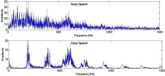
There are a number of algorithms to reduce wind noise. If the signal of speech and the noise have different frequency, the wiener filter algorithm is the best method to noise reduction that to extenuate the frequency regions where the noise is major. In the case of speech and wind noise, however, this approach leads only to limited performance, since both speech and wind noise are nonstationary broadband signals with most of the energy in the low frequency range as shown in Fig. 1 [4]. For the least squares sense to delete noise from a signal, given that the signal and noise are independent, changeless processes, the wiener filter algorithm is a good filter. It also supposes that the second order statistical of the signal and noise processes are known and acts by extenuating frequencies where the noise is expected to be the most major. The biggest problem with this method is that it assumes stationary signals, which is obviously not a good approximation for speech and wind noise.

heard as musical tones and is often called musical noise [5]. If musical noise was in the audio output of the algorithm should try to reduce this type of noise.

In section II, summarizes the performance of the algorithm NNSC explain and in section III, we develop techniques to add to the previous algorithm shows better performance in output. Thevalues oftheparameters andcompare themwith thesignal to noise ratioare showninsection IV. In the next section the performance of the proposed algorithm with other algorithms based on two parameters SNR and PESQ compared. Finally, the last section is the conclusion of this paper.

Fig. 1 This photo shows average spectrum of speech and wind noise. Both speechand wind noise are broad-band signals with most of the energy inthe low frequency range. The spectra are computed using the Burgmethod based on a few seconds of recorded wind noise and a fewseconds of speech from four different speakers.

Fig. 2 Example the result of the algorithm. II.BACKGROUND

There is a full description of the nonnegative sparse coding algorithm in paper [1]. But here we offer a brief description of the algorithm.

Assume that we observe data in the form of a large number of i.i.d . random vectors xn, where n is the sample index. Arranging these into the columns of a matrix X, then linear decompositions describe this data as X ≈ AS.

The matrix A is called the mixing matrix, and contains as its columns the basis vectors (features) of the decomposition. The rows of S contain the corresponding hidden components that give the contribution of each basis vector in the input

-70

-60

-50

-40

-30

-20

-10

0 10 20

0 2000 4000 6000 8000 10000

P

o

we

r (

d

B

)

Frequency (Hz) Speech

vectors. Although some decompositions provide an exact reconstruction of the data (i.e. X = AS) the ones that we shall consider here are approximative in nature [6].

In linear sparse coding [7, 8], the goal is to find a decomposition in which the hidden components are sparse, meaning that they have probability densities which are highly peaked at zero and have heavy tails. This basically means that any given input vector can be well represented using only a few significantly nonzero hidden coefficients. Combining the goal of small reconstruction error with that of sparseness, one can arrive at the following objective function to be minimized [7, 8]:

C(A,S) = 1/2 || X – AS ||2+ λ ∑ij f(Sij) (1)

Where the squared matrix norm is simply the summed squared value of the elements, i.e. ||X – AS||2 = ∑ij [Xij –

(AS)ij]2. The tradeoff between sparseness and accurate reconstruction is controlled by the parameter λ, whereas the

form of f defines how sparseness is measured. To achieve a sparse code, the form of f must be chosen correctly: A typical choice is f(s) = |s|, although often similar functions that exhibit smoother behaviour at zero are chosen for numerical stability.

There is one important problem with this objective: as f typically is a strictly increasing function of the absolute value of its argument (i.e. f(s1) > f(s2) if arid only if |s1| > |s2|), the objective can always be decreased by simply scaling up

A and correspondingly scaling down S. This is because setting A := αA and S := 1/α S with α > 1, does not alter the

first term in (1) but always decreases the second term. The consequences of this are that optimization of (1) with respect to both A and S leads to the elements of A growing (in absolute value) without bounds whereas S tends to zero. More importantly, the solution found does not depend on the second term of the objective as it, can always he eliminated by this scaling trick. In other words, some constraint on the scales of A or S is needed. Olshausen and Field [8] used an adaptive method to ensure that the hidden components had unit variance (effectively fixing the norm of the rows of S), whereas Harpur [9] fixed the norms of the columns of A.

With either of the above scale constraints the objective (1) is well-behaved and its minimization can produce useful decompositions of many types of data. For example, it was shown in [8] that applying this method to image data yielded features closely resembling simple-cell receptive fields in the mammalian primary visual cortex. The learned decomposition is also similar to wavelet decompositions, implying that it could be useful in applications where wavelets have been successfully applied.

III.OPTIMIZATION ALGORITHM

In this section we will discuss a few points which optimize performance and speed of implementation of the algorithm.Magnitude spectrogram of the noisy signal is calculated as follows.

D = E + F (2)

Where D is the magnitude spectrogram of the noisy signal, E is the magnitude spectrogram of the speech, F is the magnitude spectrogram of the wind noise.

In calculating the magnitude spectrogram of the noisy signal (2) if the magnitude spectrogram of the speech and the magnitude spectrogram of the wind noise increase, noise is estimated to be better than before. If the levels rise too high, the algorithm does not work well.

We add a filter to remove noise other than the wind. This filters out the frequencies of the speech signal before running the NNSC algorithm works.

Another thing that increases the speed of the algorithm is that the unit matrix factorization is a farce.

The method of minimizing the sparse cost function given in this paper is using multiplicative update rules that are derived from the gradient descent method.

IV.EXPERIMENTAL RESULTS

To evaluate the output of the algorithm, we set the input to it. Characteristics of audio files into the algorithm as follows:

In this test, including ten different files from database TIMIT are used. With the air blowing at microphone mobile, wind noise is recorded. To better estimate the noise dictionary, the total length of the audio file noise used. The sound files used in this test are equal in terms of gender. The speech signals were normalized to unit variance. The signals were sampled at 32 kHz and the short-time Fourier transform (STFT) were computed with a 64ms Hanning window and 80% overlap. We mixed speech and wind noise at signal-to noise ratios (SNR) of 6 dB. In experiments, our algorithm stopswhenthe relative change in the squared error was less than 10−4 or at a maximum of 700 iterations. As for most nonnegative matrix factorization methods, the NNSC algorithm is prone to finding local minima and thus a suitable multi-start or multi-layer approach could be used [10]. In practice, however, we obtained good solutions using only a single run of the NNSC algorithm. The algorithm is written in MATLAB programming environment.

A.Sensitive parameters affecting the output

By placing different values of some parameters in relation with paper [1], the signal to noise ratio is increased more than before.

In paper [1], the parameters are fully presented. So we just introduce briefly the parameters and the results are displayed and compared with previous results.

γ ∈ {0.7, 0.8, 0.9, 1.0}: Exponent of the short time Fourier transform. The best performance is achieved around γ =

0.8.As a result, the influence of this parameter in the signal to noise ratio is shown in Fig 3.

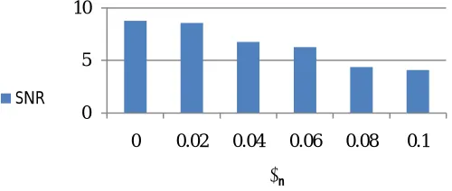
λn∈ {0.2, 0.5, 0.7}: Sparsity parameter for the precomputation of the wind noise dictionary. Given the overlap window

Hanning, bigger than before and the estimated noise level is increased. So without distorting the speech signal, the value of this parameter is increased from 0.2 in [1] to 0.4.As a result, the influence of this parameter in the signal to noise ratio is shown in Fig 4.

Ns∈ {64, 128, 256}: The number of components in the speech dictionary. In the paper [1] considered this parameter

equal 64. New microphones are sampled more, if we use the value 64, Wind noise is dominant in the speech signal and the output quality is not good. Since the phone's processing power has increased significantly and we optimized the performance of the algorithm. Increasing the number of samples doesn't slow the performance of the algorithm. Therefore, we use the value of 128 for the number of components in the speech dictionary.As a result, the influence of this parameter in the signal to noise ratio is shown in Fig 5.

Nn∈ {4, 16, 64}: The number of components in the wind noise dictionary. The large number of samples in the new

microphone will be better quality. Therefore, the number of noise components, increased than before. On the other hand, the sampling frequency is doubled. We find the value of this parameter should at least be 16. Increasing this parameter reduces the quality of the output.As a result, the influence of this parameter in the signal to noise ratio is shown in Fig 6.

ℓs∈ {0.02, 0.05, 0.1}: The sparsity parameter used for the speech code during separation. The value of this parameter

by measuring the signal-to-noise quality factor cannot be identified. Increasing this parameter reduces the noise but distorts the speech signal. This parameter balances residual noise and distortion similar to the sparsity parameter used for estimating the wind dictionary. The impact parameter Ls is determined by listening to the output. The best value for

this parameter ℓs = 0.05 is obtained.As a result, the influence of this parameter in the signal to noise ratio is shown in

Fig 7.

ℓn ∈ {0, 0.1}: The sparsity parameter used for the noise code during separation. The value of this parameter is very

B.Show parameter values versus signal to noise ratio

We have 648 different combinations to get the best values of the parameters on the audio files test. Average results for each parameter versus the signal to noise ratio is shown in the following figures.

Fig. 3 Exponent of the short time Fourier transform versus signal to noise ratio.

Fig. 4 Sparsity parameter for the precomputation of the wind noise dictionary versus signal to noise ratio.

Fig. 5 Number of components in the speech dictionary versus signal to noise ratio.

Fig. 6 Number of components in the wind noise dictionary versussignal to noise ratio. 7

8 9 10

0.2 0.3 0.4 0.5 0.6

λn

SNR

0 5 10 15

2 4 8 16 32 64 128 256 512 1024

Ns

SNR

0 5 10

0.4 0.6 0.8 1 1.2 1.4 1.6 1.8 2

ɣ

SNR

0 5 10 15

1 2 4 8 16 32 64 128 256 512

Nn

Fig. 7 Sparsity parameter for the speech versus signal to noise ratio.

Fig. 8 Sparsity parameter for the noise versus signal to noise ratio.

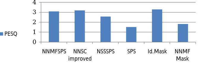
V. COMPARE THE RESULTS WITH OTHER METHODS

We compared improved method NNSC for wind noise reduction to five other noise reduction methods. Algorithms are tested over 100 audio files that have noise. Audio files recorded by Mrs. We mixed the speech with wind noise at signal to noise ratios in 0dB. Other algorithms parameters were similar to previous experiments. Algorithms are compared with our algorithm are as follows:

SPS is the spectral subtraction algorithm.

NNMFSPS is the nonnegative matrix factorization algorithm with the generalized spectral subtraction. IDEAL MASK is the ideal binary mask calculated from the original speech and noise files.

NNMF MASK is the binary mask calculated from the NNMF factorization.

NSSSPS is the nonstationary spectral subtraction algorithm with the generalized spectral subtraction algorithm optimized.

SNR and PESQ are factors to assess the quality of the output signal. You can see SNR results in Fig. 9 and PESQ results in Fig. 10.

8 8.5 9 9.5

0 0.02 0.05 0.06 0.08 0.1

ℓs

SNR

0 5 10

0 0.02 0.04 0.06 0.08 0.1

ℓn

Fig. 9 This picture shows the SNR results on all methods for the 0dB dataset.

Fig. 10 This pictureshows the PESQ value for the 4 different methods and 2 binary mask separations on the 0dB dataset.

VI.CONCLUSION

We were optimized NNSC algorithm parameters for better performance. Parameter optimization leads to better estimate the noise dictionary. By comparing the values of SNR and PESQ performance of our algorithm with other algorithms can be seen as well. Apart from id.mask our algorithm is better than others. Another possible result is that algorithm is not slowed by increasing the number of samples and the reason is that the algorithm has been optimized and faster processor. If the algorithm codes written by C++, it certainly works faster and we do this in the future.

REFERENCES

[1] M. N. Schmidt, J. Larsen, Fu-Tien Hsiao, “Wind Noise Reduction using Non-Negative Sparse Coding,” Machine Learning for Signal Processing, 2007 IEEE Workshop, pp. 431-436, Aug 2007.

[2] J.B. Miller, K.T. Andersen, and B. Hansen, “Signal processing for reduction of wind noise. Polytechnical Midterm Project,” IMM, Technical University of Denmark, Jan 2006.

[3] ITU-T. P.862 : Perceptual evaluation of speech quality (pesq): An objective method for end-to-end speech quality assessment of narrow-band telephone networks and speech codecs. http://www.itu.int/rec/T-REC-P.862/en.

[4] N. Wiener, Extrapolation, Interpolation and Smoothing of Stationary Times Series, New York: Wiley, 1949.

[5] R.Schwartz, M.Berouti, J.Mokhoul, “Enhancement of speech corrupted by acoustic noise,” Proc ICASSP, pp. 208-211, 1979.

[6] P. O. Hoyer, “Non-negative sparse coding,” Neural Networks for Signal Processing, Proceedings of the 2002 12th IEEE Workshop, pp. 557-565, 2002.

[7] G.F. Harpur, R.W. Prager, “development of low entropy coding in a recurrent network,” Network: Computation in Neural Systems, vol. 7, pp. 277-284, 1996.

[8] B.A. Olshauscn, D.j. Field, “Emergence of simple-cell receptive field properties by learning a sparse code for natural images,” Nature, vol. 381, pp. 607-609, 1996.

[9] G.F. Harpur, Low Entropy Coding with Unsupervised Neural Networks, Ph.D. thesis, University of Cambridge, 1997. [10] A.Cichocki, R.Zdunek, “Multilayer nonnegative matrix factorization,” Electronic Letters, vol. 42, no. 16, pp. 947-958, 2006.

[11] J. Kim, H. Park, “Toward Faster Nonnegative Matrix Factorization: A New Algorithm and Comparisons,” Eighth IEEE International conference on Data Mining, pp. 353-362, Dec 2008.

0 5 10 15 20

NNMFSPS NNSC

improved

NSSSPS SPS Id.Mask NNMF Mask

SNR(dB

(

0 1 2 3 4

NNMFSPS NNSC

improved

NSSSPS SPS Id.Mask NNMF