Available online: https://edupediapublications.org/journals/index.php/IJR/ P a g e | 538
An Advanced Image Denoising Using Low Rank Matrix
Decomposition for Multi-Channel Parallel MRI
STUDENT DETAILS:
KORADA MANIKANTA
M.Tech(DECS), Department of ECE
Abstract— MRI is a extensively used diagnostic tool, that gives unmatched propensity to image soft tissue. Denoising in resonance imaging (MRI) may well be a important issue and very important for clinical identification and computerized analysis. Parallel imaging is a robust method for accelerating the acquisition of magnetic resonance imaging (MRI) data, and has made possible many new applications of MR imaging.Increasing the robustness of magnetic fields can improve the signal-noise-ratio (SNR)[10][11], but will introduce radio frequency-inhomogeneity artifacts and demand high costs as a results of the noise attenuation wants high power supply devices to rise the super conduction effect t[1]. employing a multi-channel coil array to simultaneously receive MR k-space (i.e., the spatial Fourier work on domain of imaging object) signals shows vital SNR gain. Moreover, further k-space info from these coils is employed to fill uniformly under sampled k-space by utilizing parallel tomography (pMRI) techniques which can shorten MR scanning time. Even so, noise amplification and aliasing artifacts are serious in pMRI reconstructed image at high under sampling parameters [2]. Parallel resonance imaging (pMRI) techniques can intensify MRI scan through a multi-channel coil array receiving signal at an equivalent time .Reduction of noise and enhancing the images were in spatial domain increases the scope of information in the image. Then, noise and aliasing artifacts are removed from the structured matrix by applying sparse and low rank matrix decomposition technique. These also helps in reducing the non-linear artifacts. That is sparsity of the image. Nevertheless, noise amplification and aliasing artifacts are serious in pMRI reconstructed images at high accelerations. Here a low rank matrix decomposition helps in denoising the medical images using ADMM Algorithm, but was not very much efficient in reducing the error rate. So, redundant multi-resolution decomposition helps in increasing the information levels of the image. And those values were shown using performance parameters peak signal noise rate (PSNR) and structural similarity index matrix (SSIM) entropy i.e, information of an image.Using the concept of compressed sensing theory we have applied low matrix decomposition for noise removal from PMRI Images. The concept of low matrix decomposition is depends on self similarity concept. In this method we have successfully applied low matrix decomposition method along with the concept of gra
KEYWORDS: Denoising, low rank, matrix decomposition, multi-channel coil, parallel MRI .
GUIDE DETAILS:
D A TATAJEE Assistant Professor
Department of ECE
I. INTRODUCTION
Denoising in magnetic resonance imaging (MRI) is a critical issue and important for clinical diagnosis and computerized analysis. Increasing the strength of magnetic fields can improve the signal-noise-ratio (SNR), but will in-troduce radiofrequency-inhomogeneity artifacts and demand high costs because the noise attenuation requires high power supply devices to increase the superconduction effect [1]. Us-ing a multi-channel coil array to simultaneously receive MR k-space (i.e., the spatial Fourier transform domain of imaging object) signals shows significant SNR gain [2], [3]. More-over, additional k-space data from these coils can be used to fill uniformly undersampled k-space by utilizing parallel MRI (pMRI) techniques [4], [5] that can shorten MR scanning time. Nevertheless, noise amplification and aliasing artifacts are serious in pMRI reconstructed image at high undersampling factors [6]. Therefore, it is necessary to introduce a denoising procedure to improve the quality of pMRI image.
Numerous denoising methods have been proposed to re-move the noise in single MR image [7]–[11]. For example, Aja-Fernández et al. introduced the Linear Minimum Mean Square Error (LMMSE) estimator to deal with the Rician distributed noise in MR magnitude image [7]. Manjón et al.
Available online: https://edupediapublications.org/journals/index.php/IJR/ P a g e | 539 Recently, low-rank matrix completion derived from
com-pressed sensing theory [14] has been successfully applied to various matrix completion problems, e.g., image compression [15], video denoising [13] and dynamic MRI [16]–[18]. Com-pared with classical denoising methods, denoising methods based on low rank completion enforce fewer external assump-tions on noise distribution [13]. These methods rely on the self-similarity of three dimensions (3-D) images across different slices or frames to construct a low rank matrix. Nonetheless, significantly varying contents between different slices or frames may lead an exception to the assumption of low-rank 3-D images, and discount the effectiveness of these methods.
In this paper, we propose to remove both noise and alias-ing artifacts in pMRI image by usalias-ing a sparse and low rank decomposition method. By exploiting the self-similarity be-tween multi-channel coil images and inside themselves, we formulated the denoising of pMRI image as a non-smooth
convex optimization problem that minimizes a combination of
nuclear norm and l1-norm. The proposed problem is efficiently solved by using the alternating direction method of multipliers (ADMM) [19]. Experimental results of phantom
and in vivo brain imaging are provided to demonstrate the
performance of the proposed method, with comparisons to the related denoising methods.
II. Image Gradient
A. Self-Similarity in Multi-Channel Coil Images
When an L-channel coil array is used to receive MR k-space signals with Nyquist sampling rate, L coil images with
An image gradient is a directional change in the intensity or color in an image. Image gradients may be used to extract information from images.
In graphics software for digital image editing, the term gradient or color gradient is used for a gradual blend of color which can be considered as an even gradation from low to high values, as used from white to black in the images to the right. Another name for this is color progression.
Mathematically, the gradient of a two-variable function (here the image intensity function) at each image point is a 2D vectorwith the components given by the derivatives in the horizontal and vertical directions. At each image point, the gradient vector points in the direction of largest possible intensity increase, and the length of the gradient vector corresponds to the rate of change in that direction.
Since the intensity function of a digital image is only known at discrete points, derivatives of this function cannot be
defined unless we assume that there is an
underlying continuous intensity function which has been sampled at the image points. With some additional assumptions, the derivative of the continuous intensity function can be computed as a function on the sampled intensity function, i.e., the digital image. Approximations of these derivative functions can be defined at varying degrees of accuracy. The most common way to approximate the image gradient is to convolve an image with a kernel, such as the Sobel operator or Prewitt operator.
The gradient of the image is one of the fundamental building blocks in image processing. For example the Canny edge detector uses image gradient for edge detection.
Image gradients are often utilized in maps and other visual representations of data in order to convey additional information. GIS tools use color progressions to indicate elevationand population density, among others.
Image gradients can be used to extract information from images. Gradient images are created from the original image (generally by convolving with a filter, one of the simplest
being the Sobel filter) for this purpose. Each pixel of a gradient image measures the change in intensity of that same point in the original image, in a given direction. To get the full range of direction, gradient images in the x and y directions are computed.
One of the most common uses is in edge detection. After gradient images have been computed, pixels with large gradient values become possible edge pixels. The pixels with the largest gradient values in the direction of the gradient become edge pixels, and edges may be traced in the direction perpendicular to the gradient direction. One example of an edge detection algorithm that uses gradients is the Canny edge detector.
Image gradients can also be used for robust feature and texture matching. Different lighting or camera properties can cause two images of the same scene to have drastically different pixel values. This can cause matching algorithms to fail to match very similar or identical features. One way to solve this is to compute texture or feature signatures based on gradient images computed from the original images. These gradients are less susceptible to lighting and camera changes, so matching errors are reduced.
The gradient of an image is given by the formula:
,
Available online: https://edupediapublications.org/journals/index.php/IJR/ P a g e | 540 The gradient direction can be calculated by
the formula:[1]:706
.
For example, to calculate we apply a
1-dimensional filter to the image by convolution:
where denotes the
1-dimensional convolution operation. This 2×1 filter will shift the image by half a pixel. To avoid this, the following 3×1 filter
can be used.
B. Denoising in pMRI by Low Rank Matrix Decomposition
To remove noise and aliasing artifacts simultaneously, we ap-proximately model the noisy image of pMRI as a superposition
Fig. 1. (a) Phantom reference image reconstructed with 32-channels full k-space data. (b) Image reconstructed by a representative k-k-space based pMRI reconstruction algorithm. (c) Difference image between (a) and (b). (d) Sorted singular values of a patch stack in the resulting image of (b) are more and larger than those of (a).
of clear image, aliasing artifacts and noise. Thus, each matched patch matrix P from pMRI reconstructed coil images can be decomposed as
P = C + D + N (4)
where matrix C represents the original noise-free image, which is low rank due to the self-similarity of multi-channel coil images. Matrix D represents residual aliasing artifacts and has a sparse structure, matrix N indicates random image noise that is generally introduced in the acquisition phase and amplified in the pMRI reconstruction process [4], [5]. Because the self-similarity and sparseness can be, respectively
characterized by means of rank and l0 norm, denoising of coil
images can be described as a matrix decomposition problem that extracts the clear image C from the observed image P by solving the following minimization problem:
min rank(C) + λ D
0
C,D
s.t. P − C − D F ≤ δ (5)
where 0 denotes l0 norm that accounts the number of non-zero
entries in matrix or vector, F denotes Frobenious norm for matrix, λ > 0 is a tuning parameter providing a tradeoff between sparse and low-rank components, and δ reflects the level of noise in observation P . Generalizations of (5) are often intractable
because rank and l0 norm are nonconvex functions, we instead consider a convex relaxation of (5), which has also been proven to promote low-rank solutions [21]
min
C ∗+ λ D 1
C,D
s.t. P − C − D F ≤ δ (6)
where C∗ represents the nuclear norm of matrix C (i.e., the sum
of its singular values), and 1 is the summation of l1 norms over all matrix columns. Eq. (6) can be solved with an efficient ADMM method by taking full advantage of its separate structure, which is detailed in the following subsection.
It should be noted that (6) only recoveries the pixels within one patch of individual coil image. The denoising of entire coil image can be accomplished by sliding the patch across entire image in a raster fashion. Thus, each pixel is calculated repeatedly between overlapping patches and obtains multiple estimations. The final output of each pixel is calculated by simply averaging all estimates of this pixel from overlapping patches.
C. Optimization Algorithm
In this paper, we introduce the augmented Lagrange alter-nating direction method (ADMM) [19] for solving non-smooth convex optimization problem (6). The augmented Lagrange function of (6) is defined as
LA(C, D, Z) = λ D 1+ C ∗ − Z, C + D − P
+ β
C + D − P F2 (7)
2
where β > 0 is the penalty parameter for the violation of the linear constraint and Z is the Lagrange multiplier of the linear constraint, and · denotes the standard trace inner product operator. The minimization task (7) can be split into three easier subproblems as follows:
Dk+1∈arg min LA(D, Ck, Zk)
)
(8)Ck+1 arg min A(D k+1
, C, Z
Zk+1=Zkγβ(Dk+1+Ck+1 k P )
∈
− L
−
Available online: https://edupediapublications.org/journals/index.php/IJR/ P a g e | 541 do
1. Compute Dk+1
Dk+1 = βZk
−Ck
+ P−TΩ∞λ/β β Zk
−Ck +P 1 1
where TΩ∞λ/β denotes the Euclidean projection onto
Ωλ/β : {
X
∈ n×n | − λ/β ≤ x i,j
≤
λ/β}
∞
2. Compute Ck+1
C
k+1 = Uk+1diag max σi k+1− 1
, 0 (Vk+1)
T
β
where Uk+1, Vk+1, and{σk+1} generated by the singular
values decomposition of P−Dk+1 + (1/β)Zk
3. Updata the Zk+1
√
Zk+1= Zk − γβ(Dk+1+ Ck+1 − P ), γ ∈0,
5 + 1
2until converged
TABLE I
SUMMARY OF EXPERIMENTAL DATA SETS
√
where γ ∈ (0, ( 5 + 1)/2) is a relaxation factor to guarantee convergence of iterations. The variables C, D, and Z are minimized separately, and each of them has a closed-form solution. The detail procedure for solving the problem (8) is described in Algorithm 1.
III. EXPERIMENTAL RESULTS AND DISCUSSIONS
A. Source Data
The performance of the proposed method was validated using three scanned data sets acquired on a 3T whole-body scanner. Both phantom and in vivo data sets were fully sampled on the scanner and later undersampled on the computer to mimic the clinical pMRI acquisition. A brief description of all data sets is summarized in Table I.
Noisy images were generated from the undersampled k-space data with generalized auto-calibrating partially parallel acquisitions (GRAPPA) [5] that is the most widely used pMRI reconstruction method in commercial MR scanners. Images reconstructed with full k-space data were used as the pseudo ground truths.
C. Algorithm Implementation
The proposed algorithm was compared against some recently developed methods used for MRI denoising: LMMSE [7], block method of 4-dimension denoising (BM4-D) [10], and ANLM [9]. All denoising results of these benchmarks methods were generated from the source code or executable released by their authors. For a fair comparison, an 8 × 8 patch was adopted in the implementations of all methods, and the spatial search radius was 20 pixels. LMMSE was applied on the single noisy image, while other filters were directly applied on noisy coil images where the coil direction was approximately in place of volumetric direction for BM4-D and AONLM, then the denoised coil images were combined into final ones in a sum-of-squares fashion [22].
For the proposed method, the parameter λ was set following
[23]: λ = 1/ max(M2, K). The parameter β was empiri-cally
set to 0.25M2K/σ P1 for convenience, where σ = mode(σP )
is the unbiased local standard deviation for each group of matching image patches. The relaxation factor γ was set to 1.6 for the updating of Lagrange multiplier. To guarantee the convergence of the proposed algorithm, the relative change at each iteration was calculated
ξ = (Dk, Ck)−F + 1 .
(Dk+1, Ck+1) (Dk, Ck)
The stopping criterion was either the tolerance ξ < 5e− 6 or the maximal number of iterations 20 being reached. Both image reconstruction and denoising were performed in Matlab (MathWorks, Natick MA) on a windows 7 computer equipped with an Intel Celeron G540, 2.50 GHz CPU and 4 GB RAM.
B. Quality Measures
Two quality measures were used for quantitatively evaluating the accuracy of denoised results. The first is the Peak signal noise rate (PSNR) metric, which is formed by
calculating the ratio between the maximum possible power of a signal and the power of corrupting noise that affects the fidelity of its representation
max(Iref )
PSNR
= 20 log
Available online: https://edupediapublications.org/journals/index.php/IJR/ P a g e | 542 where Irecon and Iref represent denoised image and noiseless
reference image, respectively.
Another quality measure was the structural similarity index matrix (SSIM) [24] which better relates to the human visual system than conventional metrics based on the mean squared error. The SSIM between two images I and J is given by
1 (2μiμˆj + c1)(2σi,j + c2)
SSIM(I,J ) =
N μi2+ μˆj2+1 c σi2+ σj2+ c2 i I,j J
where μi and μˆj are the respective local mean values, σi and σj
the respective standard deviations, σi,j covariance value, c1
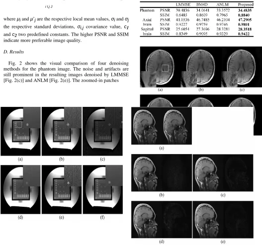
and c2 two predefined constants. The higher PSNR and SSIM indicate more preferable image quality.
D. Results
Fig. 2 shows the visual comparison of four denoising methods for the phantom image. The noise and artifacts are still prominent in the resulting images denoised by LMMSE [Fig. 2(c)] and ANLM [Fig. 2(e)]. The zoomed-in patches
Fig. 3. Example denoising results for a sagittal brain data set. (a) Reference image and noisy image generated by pMRI with an undersampling factor of 6. The noisy image is filtered by (b) LMMSE, (c) BM4-D, (d) ANLM, and (e) the proposed method. The difference images between the reference image with filtered images are shown at the right of each denoised image.
TABLE II
Available online: https://edupediapublications.org/journals/index.php/IJR/ P a g e | 543 shows the residual artifacts are retained in the filtered images of
LMMSE, BM4-D, and ANLM. In contrast, both noise and residual artifacts are removed in the denoised image by the proposed method at a little sacrifice of image contrast. Note that the noise in the background region of LMMSE denoised image is amplified, the similar phenomenon was observed in previous literature [7]. This is because the standard deviation of noise is automatically estimated in LMMSE according to the background noise, which ignores the spatially varying noise.
Fig. 3 shows the filtered images of sagittal brain data set by the four denoising methods and corresponding difference images. All methods show good behaviors on noise suppres-sion. The noise level in the image of LMMSE is slightly
higher than those in other results, which can be observed from the difference image and the numeric comparisons listed in Table II. Nevertheless, the anatomical details are sacrificed in the images denoised by all the patch based methods especially for the result of BM4-D [Fig. 3(c)]. The proposed method produces a satisfactory balance between noise cleaning and edge preservation among the three patches based methods.
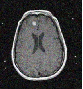
Fig. 4 illustrates the resulting images of axial brain data set by the four denoising methods. The local images are zoomed in and listed in the left-bottom of the denoised images, respec-tively. The intractable noise is visible in the center of the image denoised by LMMSE, and as is observed in Fig. 2, noise is
Fig. 4. Example denoising results for an axial brain data set. (a) Reference image. (b) Noisy image generated by pMRI with an undersampling factor of 6. (c) LMMSE denoising. (d) BM4-D denoising. (e) ANLM denoising.
(f) Denoised by the proposed method. A region of interest was zoomed in (enclosed by a white rectangle in the reference image) and shown at the bottom-left corner of each resulting image.
TABLE III
TIME EXHAUSTS OF DENOISING METHODS IN EXPERIMENTS (SEC.)
amplified at the corners of image caused by the over-estimation of noise standard deviation. The zoomed in patch shows ANLM has a more conservative behavior on noise suppression than BM4-D and the proposed method. Although the image filtered by the proposed method appears to be slightly oversmoothed, the zoomed-in patch image shows the proposed method pre-serves most of the important features in the filtered image. The aliasing artifacts are weaker in the image denoised by the proposed method than those of LMMSE and BM4-D.
Results of quantitative evaluation are reported in Table II. The highest PSNR and SSIM values are highlighted in each cell to facilitate the comparison. As shown, the proposed method outperforms other approaches in all cases.
Table III lists the computational times of all denoising methods in experiments. LMMSE which was directly applied on single noisy image has the shortest denoising time. The proposed method has the longest time among all denoising methods; however, it can still meet the real-time requirements in clinical applications by implementing the proposed algorithm in C programming language.
IV. Experimental Results
Using the concept of compressed sensing theory we have applied low matrix decomposition for noise removal from PMRI Images. The concept of low matrix decomposition is depends on self similarity concept. In this method we have successfully applied low matrix decomposition method along with the concept of gradient techniques to efficiently remove the noise from the PMRI images.
Below is the experimental results implemented using MATLAB software.
Above figure represents the MRI image of human brain and below figure represents atifact and noise effected image. Generally these artifacts and noise are generated inhomogeneity between radio frequency signals and high under sampling factors.
Available online: https://edupediapublications.org/journals/index.php/IJR/ P a g e | 544 Since we are decomposing the entire image using we can
effectively reduce the noise level compared to any other previous techniques. Here based on the background noise adjustment we can effectively estimate the standard deviation value of noise for entire image.
In our proposed method the aliasing artifacts are becomes weaker due to low matrix decomposition which leads to effectively and efficiently removes the noise and gradient technique is used to preserve the edges of the image.
Below are the MATLAB simulation results .
V.CONCLUSION
We have described a novel denoising method for pMRI by exploiting the self-similarity between multi-channel coil images and inside themselves. The proposed method simul-taneously removes noise and aliasing artifacts by leveraging sparse and low rank matrix factorization. Experimental re-sults demonstrate that the proposed algorithm can benefit both visual diagnostic and quantitative methodologies. The proposed method could be extended to multiple dimensions imaging by exploiting the redundancy and similarity between multi-slice and multi-frame images to achieve a higher SNR gain that is warranted in a future study.
REFERENCES
[1] H. Wada et al., “Prospect of high-field MRI,” IEEE Trans. Appl. Supercond., vol. 20, no. 3, pp. 115–122, Jun. 2010.
[2] S. M. Wright, R. L. Magin, and J. R. Kelton, “Arrays of mutually coupled receiver coils: Theory and application,” Magn. Resonance Med., vol. 17, no. 1, pp. 252–268, Jan. 1991.
[3] J. Wosik et al., “Superconducting single and phased-array probes for clinical and research MRI,” IEEE Trans. Appl. Supercond., vol. 13, no. 2,
pp.1050–1055, Jun. 2003.
[4] K. P. Pruessmann, M. Weiger, M. B. Scheidegger, and P. Boesiger, “SENSE: Sensitivity encoding for fast MRI,” Magn. Resonance Med., vol. 42, no. 5, pp. 952–962, Nov. 1999.
[5] M. A. Griswold et al., “Generalized autocalibrating partially parallel ac-quisitions (GRAPPA),” Magn. Resonance Med., vol. 47, no. 6, pp. 1202– 1210, Jun. 2002.
[6] A. Deshmane, V. Gulani, M. A. Griswold, and N. Seiberlich, “Parallel MR imaging,” J. Magn. Resonance Imag., vol. 36, no. 1, pp. 55–72, Jul. 2012. [7] S. Aja-Fernández, C. Alberola-López, and C.-F. Westin, “Noise and
signal estimation in magnitude MRI and Rician distributed images: A LMMSE approach,” IEEE Trans. Image Process., vol. 17, no. 8, pp. 1383–1398, Aug. 2008.
[8] H. Liu, C. Yang, N. Pan, E. Song, and R. Green, “Denoising 3-D MR images by the enhanced non-local means filter for Rician noise,” Magn. Resonance Imag., vol. 28, no. 10, pp. 1485–1496, Dec. 2010.
[9] J. V. Manjón, P. Coupé, L. Martí-Bonmatí, D. L. Collins, and M. Robles, “Adaptive non-local means denoising of MR images with spatially vary-ing noise levels,” J. Magn. Resonance Imag., vol. 31, no. 1, pp. 192–203, Jan. 2010.
[10] M. Maggioni, V. Katkovnik, K. Egiazarian, and A. Foi, “A nonlocal transform-domain filter for volumetric data denoising and reconstruction,” IEEE Trans. Image Process., vol. 22, no. 1, pp. 119–133, Jan. 2013. [11] S. Aja-Fernandez, V. Brion, and A. Tristan-Vega, “Effective noise
es-timation and filtering from correlated multiple-coil MR data,” Magn. Resonance Imag., vol. 31, no. 2, pp. 272–285, Feb. 2013.
[12] D. J. Larkman and R. G. Nunes, “Parallel magnetic resonance imaging,”
Phys. Med. Biol., vol. 52, no. 7, pp. R15–R55, Apr. 7, 2007.
[13] H. Ji, C. Liu, Z. Shen, and Y. Xu, “Robust video denoising using low rank matrix completion,” in Proc. IEEE Conf. CVPR, 2010, pp. 1791–1798. [14] D. L. Donoho, “Compressed sensing,” IEEE Trans. Inf. Theory, vol. 52,
no. 4, pp. 1289–1306, Apr. 2006.
[15] G. Gilboa and S. Osher, “Nonlocal operators with applications to image processing,” Multiscale Model. Simul., vol. 7, no. 3, pp. 1005–1028, Apr. 2008.
[16] S. G. Lingala, H. Yue, E. Dibella, and M. Jacob, “Accelerated dynamic MRI exploiting sparsity and low-rank structure: k-t SLR,” IEEE Trans. Med. Imag., vol. 30, no. 5, pp. 1042–1054, May 2011.
[17] A. Majumdar, “Improved dynamic MRI reconstruction by exploiting spar-sity and rank-deficiency,” Magn. Resonance Imag., vol. 31, no. 5, pp. 789– 795, Jun. 2013.
[18] X. X. Yin, B. W. Ng, K. Ramamohanarao, A. Baghai-Wadji, and D. Abbott, “Exploiting sparsity and low-rank structure for the recovery of multi-slice breast MRIs with reduced sampling error,” Med. Biol. Eng. Comput., vol. 50, no. 9, pp. 991–1000, Sep. 2012.
[19] T. M and Y. X, “Recovering low-rank and sparse components of matrices from incomplete and noisy observations,” SIAM J. Optim., vol. 21, no. 1, pp.57–81, Jan. 2011.
[20] J. V. Manjón, P. Coupé, A. Buades, D. Louis Collins, and
M.Robles, “New methods for MRI denoising based on sparseness and self-similarity,” Med. Image Anal., vol. 16, no. 1, pp. 18–27, Jan. 2012.
[21] B. Recht, M. Fazel, and P. A. Parrilo, “Guaranteed minimum-rank solu-tions of linear matrix equasolu-tions via nuclear norm minimization,” SIAM Rev., vol. 52, no. 3, pp. 471–501, Aug. 2010.
[22] P. B. Roemer, W. A. Edelstein, C. E. Hayes, S. P. Souza, and
O.M. Mueller, “The NMR phased array,” Magn. Resonance Med., vol. 16, no. 2, pp. 192–225, Nov. 1990.
[23] E. J. Candes, X. Li, Y. Ma, and J. Wright, Robust Principal Component Analysis? Stanford, CA, USA: Stanford Univ. Press, 2009.