The Method of Variable False Tranelents for the Solution of Coupled Elliptic Equations

(1)

I

Volume 6 - Part 2 December 2005

I

ISSN 1729-5106

EAST AFRICAN

JOURNAL OF

PHYSICAL SCIENCES

1.W.

Waithaka, J. Okumu & R.L. Stangl... 89

Solution to a generalized singular Cauchy problem of the Euler Poisson Darboux equation.

I.C.C. Wanjala 101

The method of variable false transients for the solution of coupled elliptic equations.

"F.K. Gatheri 107

(2)

East African Journal of Physical Sciences 6(2): 107-116 (2005)

The method of variable false

tranelents

for the solution of coupled

elliptic

equations

Francis K. Gatheri

Department of Mathematics, School of Pure and Applied Sciences, Kenyatta University, P.O. Box 43844 - 00100, Nairobi, Kenya

Email: [email protected]

A method for the numerical solution of coupled, non-linear elliptic, partial differential equation is described. The essential feature of the formulation is the use of different false transient factors in different flow regions. In regions where velocity gradients are high, small time steps are required so that small false transient factor are used, elsewhere large time steps and false transients factors are employed. The number of iteration required for convergence was significantly reduced when compared with the conventional method. The effectiveness of the method is demonstrated by applying it to the problem of natural convection in a three-dimensional enclosure heated and cooled on one wall.

Key words: false transient factors; natural convection.

INTRODUCTION

The numerical steady state solution of convection problems may be found by either directly solving the steady equation, or by solving the unsteady equations- all but one of which become parabolic. The solution is then obtained by marching the parabolic equations through time. A reason for the difficulty in using parabolic solvers is the limit on the time step size. We have used the fact that in most flow fields the time step required to achieve stability is different in different parts of the flow field. Regions with high velocity gradients require small time steps whereas regions with low velocity gradients are stable when large time steps are used. In most solution procedures the time step used is constant throughout the computational region and is normally small in order to maintain the stability of the solution. This often results in a large number of time steps to reach convergence.

The use of variable false transient factors has the advantage of allowing the 'characteristic' time in each region to advance at the same rate. The cell Reynolds number is high near the walls where the velocity is high. The use of small values of false transient factors reduces the time step in those regions and helps to maintain the stability of the solution procedure. In the core of the cavity the flow is very weak and the cell Reynolds number is low. Large false transient factor can be applied to increase the time step in that region. This ensures that the solution procedure is stable, but, leads to a reduction of the number of iterations to reach convergence. In this paper we develop the method and show its efficiency by applying it to a natural convection problem.

The method of the false transient developed by Mallinson & de Vahl Davis (1973) has been shown to converge faster in the case of the standard problem of two-dimensional natural convection heated and cooled on opposite walls. However, for the colliding boundary layer problems, which are the concern of this paper, this method has not proved to be sufficient fast in obtaining converged solutions.

In the colliding boundary layer problem (Figure 1), we are only interested in the final steady state, and the procedure of using constant time steps in the flow field is, therefore,

(3)

108 - Gatheri, Variable false transient factors

inefficient. If the steady state solution exists and is unique, it may be obtained more efficiently by the introduction into the governing equations of variable false transient factors.

This is the basis of the method that is proposed in this paper. The variable false transient factors lead to a set of parabolic equations which are solved by marching through a distorted time; no inner iterations are involved and the rate of convergence is enhanced by the use of different time steps in different parts of the flow field, for the different equations. The true transient solution is lost, but at large times the transient terms decay and the true steady state solution is recovered.

The method discussed here has been applied to a number of natural convection problems.

For two- and three-dimensional situations, extensive tests on the accuracy and speed of the method have been performed. It was found that the method is at least an order of magnitude faster than that developed by Mallinson & de Vahl Davis (1973). Further by varying the time steps in the different flow regions for the situation shown in Figure 1 it was possible to obtain

converged solutions for Ra

>

5x 105 without switching on the turbulence model (Gatheri, 1994).

z

x

Figure 1.The solution region and coordinate orientation

MATHEMATICAL FORMULATION

A viscous conducting fluid for which the Boussinesq approximation is valid, is assumed i.e. all the thermophyical properties are taken to be constant except for the density in the buoyancy term of the momentum equation for which a linear temperature relationship is assumed. The equations governing natural convection within the cavity are presented below in non-dimensional form for an incompressible flow.

or;

-

1

2--a+Vx(r;xU)=

Gr

l/2 V r;-(Vx0g) (1)

0=V21j1+( (2)

Ge - 1 2

-

+

V.(U0)

=

1/2 V 0 (3)

a

PrGr

in which

U

is the velocity vector, the vector potential is defined by

U

=

V

xip; ~

=

V

x

U

is

the vorticity vector; 0 is the non-dimensional temperature defined by

e

=

(T - TJI

M'

where

(4)

Gatheri, Variable false transient factors - 109

KJ'

=~ -

T

w

and the subscript wand h refer to the isothermal cold window and isothermal

heater respectively (see Figure 1). The Grashof and Prandtl numbers are

Gr= gfJJ!{[ / v

2 and

Pr

=V /

a

respectively; L is the length of the room;

P

is the volumetric coefficient of expansion, v is the kinematics viscosity, K is the thermal diffusivity and g is the gravitational acceleration. Equations (1-3), together with equation [J='Vxware to be solved for the velocity and

temperature fields.

The method of the variable false transient makes two simple changes to this set of equations. Equation (2) in unchanged and reproduced here as equation (5), whereas the time derivatives in equations (1) and (3) are given modified coefficients. The equations set then becomes

1

ac;

-

1 2

---+Vx(C;XU)=-1-/2 V C;-(Vx8g) (4)

a~iJk

ot

Gr

0=

V2'1'

+f

(5)

1 tB

-

1

2

--

+

v.(ue)

= 1/2V'8 (6)

aeijk

ot

PrGr

If a steady state exits, clearly it will be reached using either set of equations. Further, the false transient factors a (ijk and aeijk' are functions of position as indicated by the subscripts i

jk:

Equation (5) is unchanged, whereas in the method described by Mallinson & de Vahl Davis (1973) a fictitious transient term was inserted to the left hand side of the equation.

We now consider the boundary conditions for these equations, which are to be solved for a three-dimensional cavity, illustrated in Figure 1.

The temperature is zero on the cold portion of the wall and unity on the hot portion of the wall. All the remaining walls are adiabatic. The boundary condition for vorticity

C

;

and vector potential are derived from the velocity boundary conditions. The walls of the enclosure are impermeable and stationary resulting in zero values for both the normal and tangential component of velocities. The boundary conditions for the vector potential derived by Hirasaki &

Hellums (1968) are used in this study. The boundary conditions for the vorticity are derived from equation (2) as outlined by Mallinson & de Vahl Davis (1977).

NUMERICAL METHODS

(5)

THE SOLUTION PROBLEM

The variable false transient method is an extension of the false transient method developed by Mallinson & de Vahl Davis (1973). However, in this method the variable false transient factors could be applied to any set of elliptic equations. The general arrangement for the solution procedure is described in Gatheri (1994).

Defining the grid cell Reynolds number as Rail

=

Iv

ilhx(i)/rCl>' where hx(i) is the mesh size

and I'II> is the diffusion coefficient; here we propose that aCl>ijk be a function of position. If

Reel/ > 2 small values are chosen. On the other hand if Reel/ < 2 a large value is chosen. For example, the simplest strategy' is to use a constant small value for aCl>ijk(aCl>L) when Reel/ > 2 and a large value when Reel/ < 2(aCl>H)' There is no clear-cut method of choosing the values of the false

transient factors. The values of the,variable false transient factors aCl>ijkdepend on the geometry of

the problem considered, the mesh size and the value of the other non-dimensional parameters. It has been found that with suitable values for the coefficient aCl>ijk' this method is superior to that

used by Mallinson

&

de Vahl Davis (1973) for three-dimensional problems (Gatheri

et al.

,

1993).

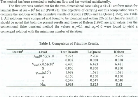
The method has been extended to turbulent flow and has worked satisfactorily.

The first test was carried out for the two-dimensional case using a 41 x41 uniform mesh for laminar flow at

Ra

=

106for air (Pr-0.71). The objective of carrying out this computation was to

compare the solution withthe primitive TP.SUltSof Kelson (1990) and Le Quere (1990), see Table 1. All solutions were compared and found to be identical and within 2% of Le Quere's result. It should be noted that both the present results and those of Kelson (1990) are grid values. For the conventional false transient method the values

a"

=0.1 and

as

=1.0 were found to yield a

converged solution with the minimum number of iteration.

Table 1. Comparison of Primitive Results.

Ra=106 41x41 Test Results LeQuere Kelson

Umax(0.5,y)x 10 2.223 2.206 2.205

y 2 0.038 0.038 0.038

Vmax(x,0.5)x10 6.470 6.483 6.481

X 0.850 0.850 0.850

\jImax(x102) 1.688 1.681 1.681

x 0.150 0.150 0.150

y 0.549 0.547 0.540

NUo 8.963 8.825 8.82

In order to determine the optimum values for the false transient factors, initial calculations were performed using various false transient factors for aSij when Re<2 (aOH)' aSij

=1

when

Re>2 (aOL) and with a 9j =

01

in the whole flow field (where the subscript

i

,

j

refers to

(6)

Gatheri, Variable false transient factors -

111

when Re<2 (a~H) and a(Ij=0.10 when Re>2 (a~L)' The results of these tests are shown in

Figures 2 and 3, respectively.

Figure 2 shows that increasing aBH enhances and increases the rate of convergence. There

is a sharp reduction in the number of iterations when aBH is increased from 1.0 to 2.0. For values

of aBH greater than 2, there is very little change however, the number of iterations to reach

convergence increases slightly.

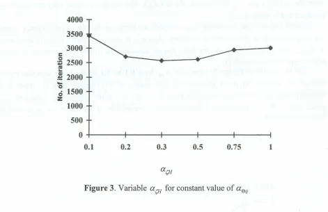
For the vorticity (Figure 3) increasing ailf from 0.1 to 0.3 resulted in a decrease in the

number of iterations to reach convergence. For values of at;H greater than 0.3 there is a

substantial increase in the number of iterations to reach convergence whereas for values of at;H

greater than 1.0 this resulted in either premature termination of the iterations or excessive

computation times.

4000

3500

3000

e

0

2500 ;:;

111

.

..

(I)

2000

~

-

0

0 1500 z

1000

500

0

1 1.5 2 3 4 5

(7)

4000

3500

3000

1000

500 o

+

-

---~----

-

+---~---+

-

----~

0.1

c

o

:w

2500

I!

cu

~ 2000

_...

o

1500

z

0.2

0.3

0.5

0.75

1

Figure 3. Variable at;H for constant value of aeij

In view of this test, both

a

(H and

a

(}H were varied and the number of iterations required to

reach steady state are given in Table 2. The result shows that there is a significant reduction of the number of iterations to reach convergence as a result of using different false transient factors in the flow field.

Table 2. Number of iteration for convergence to 10-4 for Ra

=

106

aeL aeH _a₍_L _a(H _{No of}

Rec>2 Rec~ Rec>2 Rec~ iteration

1.0 1.0 0.1 0.1 ₃₄₃₉

1.0 1.50 0.1 _0.1 ₂₅₆₉

1.0 _2.0 0.1 _0.2 ₁₄₀₉

1.0 _3.0 0.1

_OJ

₈₂₅

1.0 _3.0 0.1 0.4 ₉₆₅

1.0 _3.0 0.1 _0.5 ₁₅₁₃

1.0 _4.0 0.1 _0.5 ₁₅₈₇

(8)

Gatheri, Variable false transient factors - 113

APPLICATION TO THE COLLIDING BOUNDARY LAYER PROBLEM

Tests were conducted on the colliding boundary problem using a 21 by 21 by 21 uniform mesh

for laminar flow at Ra

=

104 and for a fluid of Prandtl number 0.71. All the solutions obtained

were compared and found to be similar to four significant figures. Decreasing the convergence

criterion by an order of magnitude and observing that the solution changed only in the fifth significant figures verified the fact that convergence was reached.

In this computation it was found thathigh values of false transient factors could be used.

For the colliding boundary layer problem, the flow has thin boundary layers along the active wall whereas the core of the cavity is thermally stratified (the majority of the cavity). As a result,

calculations were performed using various false transient factors for aeijk when Re<2 (aOH)'

aeijk

=1

when Re>2 (aoJ and with a(ijk

=

1 in the whole flow field. The calculations were then

repeated with aOL = aOH = 1 with various values of a (ljkwhen Re<2 (ai:;H) and a (ljk=0.25 when

Re>2 (a

sL)'

The results of these study are shown in Figures 4 and 5, respectively.

The use of high false transient values for the energy equation enhances and increases the

rate of convergence (Figure 4). For values of

aOH

greater than 5, very little change occurs in the

number of iterations required to reach convergence. There is more than 50% reduction in the

number of iteration required when

aOH

is varied from 1 to 5.

4500

4000

3500

c ₃₀₀₀

0

••

1\1

2500

• ..

II) :t:

-

0 2000

0

z 1500

1000

500

0

1 2 5 10 20 50 100

(9)

In the case of vorticity (Figure 5), there is a sharp decrease in the number of iterations when a~H is varied from 0.25 to 0.5. The minimum occurs at a~H=1.0. Outside the range of

2<a~H<10, a~H has little effect on the number of iterations to reach convergence and for

a~H>10, the solution diverges.

4500

4000

3500 I

g

3000

:w

~ 2500

.•.•

:s

2000

~ 1500

1000

500

O+---~---r---r_----_+----~

0.25 0.5 1 2 5 10

Figure 5. Variable ar;H for constant value ofaeijk

A similar test was performed where both a~H and aOH were varied and the number of

(10)

Gatheri, Variable false transient factors -

115

Table 3. Number of iteration and CPU time for convergence to

10 -

4

for

Ra

=

10

4

a0L a0H asL _asH No of

Rec>2 Rec~ Rec>2 Rec~ iteration CPU time

1 .

0

1 .

0

0 .

2

5

0 .

25 ₄₁₂₁

_1330.9

1 .

0 _2.0

_0.25

₁

_;

_.0

₁₀₆₁

_560.0

1 .

0 _2.0

0 .

25

1 .

5 ₁₇₉₆

_814.6

1 .

0 ₃

_.

₀

0 .

25

1 .

0 ₁₂₂₀

_544.3

1 .

0 ₅

_.

₀

_.

₂₅

1 .

0 ₁₀₄₆

_474.6

1 .

0 _5.0

0 .

25 _5.0

_~

₈₉₄

_435.0

1 .

0 _5.0

_0.25

_0.5

₁₉₂₈

_875.3

1 .

0 ₁₀

_.

₀

0 .

25

1 .

0 ₁₀₆₄

_482.7

1 .

0 _100.0

0 .

25

1 .

0 ₁₀₅₈

478 .

1

1 .

0 _100.0

0 .

2

5 _5.0

₂₅₄

91 .

7

The results in Table 2 and Table 3 are valid for the particular problem studied and a different set of false ,transient factors may be needed for other problems. For the differentially heated cavity problem it has been shown that, with suitable choice of variable false transient factors a qij and aeu this formulation is four times faster than the conventional method whereas

for the colliding boundary layer problem with suitable choice for the parameters at;ijk and aeijk,

this procedure is

10

times faster than the conventional method for the particular problem.

Conservatively, therefore, this method has proved to be at least an order of magnitude faster than the conventional method in furnishing steady state solutions for natural convection problems. The above procedure was only applied in solving parabolic equation. The development of the variable false transient method permitted the prediction of three-dimensional steady motion with a reasonable amount of computational effort.

CONCLUSION

(11)

REFERENCES

Gatheri, F.K. 1994. 'Numerical Simulation of Turbulent Natural Convection in an Enclosure.

Ph.Di.thesis, University of New South Wales, Sydney, Australia.

Gatheri, F.K., Reizes, J.A.~ Leonardi, E and de Vahl Davis, G. 1993. The use of variable false transient factors for the solution of natural convection problems. Proceeding 5th Australasian Heat and Mass Conference, Brisbane, Australia.

Haussling, H.J. 1979. Boundary-fitted coordinates for accurate numerical solution of a multi-body flow problems. Journal of Computational Physics 30: 107-124.

l-firasaki GJ and Hellums J.D. 1968. Py'general formulation of the boundary conditions on the vector potential in three-dimensional hydrodynamics. Quarterly Applied Mathematics, XXV: 331-342.

Kelson, N. 1990. The laminar boundary layers regime for natural convection of air in a square cavity. Report 1990/FMT/3, University of New South Wales, Sydney, Australia.

Le Quere, P. 1990. Accurate solutions to the square thermally driven cavity at high rayleigh number. Centre National de la Recherche Scientificicque LIMSI, Notes et Documents, Osray, France, 90-92.

Mallinson, G.D. and de Vahl Davis, G. 1973. The method of false transients for the solution of coupled elliptic equations. Journal of Computational Physics, 12: 435-461.

Mallinson, G.D. and de Vahl Davis, G. 1977. Three-dimensional convection in a box: A numerical study. Journal of Fluid Mechanics, 83: 1-31.

Samarskii, A.A. and Andreyev, V.B. 1963. On a high accuracy difference scheme for elliptic equation with several space variables. USSR Computational Mathematics and Physics, 3:

1373-1382.

. - ~'- .-.

---

-

--

-

_

.

~----;.,,---..----

--.l ..:. :• _- ~- • ~.

The Method of Variable False Tranelents for the Solution of Coupled Elliptic Equations

I

I

EAST AFRICAN

JOURNAL OF

PHYSICAL SCIENCES

Contents

1.W.