Volume 3, No. 2, March-April 2012
International Journal of Advanced Research in Computer Science
RESEARCH PAPER
Available Online at www.ijarcs.info
ISSN No. 0976-5697
Performance Analysis of Particle Swarm Optimization Algorithms for Jobs Scheduling in
Data Warehouse
S.Krishnaveni*
Ph.D (CS) Research Scholar Karpagam University, Coimbatore
Tamil Nadu, India [email protected]
M.Hemalatha
Prof. & Head, Dept. Software Systems & Research Karpagam University, Coimbatore
Tamil Nadu, India [email protected]
Abstract: The Enterprise Information System contains data warehouses frequently residing in the number of machines in at least one data center. Many jobs run to bring data into the data warehouses. Jobs are scheduled by dependency basis. Data processing jobs in the data warehouse system involve many resources, so it is necessary to find the best job-scheduling methodology. Particle Swarm Optimization (PSO) is used to find solutions easily and fruitfully, so it is employed in several optimization and search problems. Improved PSO, Hybrid Improved PSO (Improved with simulated annealing (SA)) and Hybrid PSO (three neighborhood SA algorithms are designed and combined with PSO) are used to achieve better solutions than PSO. This paper shows the use of hybrid improved PSO to scheduling multiprocessor tasks, Hybrid PSO to minimize the makespan of job-shop scheduling problem for each best solution that particle find. Algorithms are demonstrated by applying in benchmark job-shop scheduling problems. The superior results indicate the successful incorporation of PSO and SA. This survey results shows the optimal scheduling algorithm to reduce runtime and optimize usage of resources.
Keywords: HPSO, Hybrid ImPSO, ImPSO, Job Scheduling, Particle Swarm Algorithm, Simulated Annealing
I. INTRODUCTION
In Enterprise Information System, scheduling is most important one. It’s used in various fields like production planning, transportation, logistics, communications and information processing. In operating system, job scheduling is an optimization problem and the jobs are assigned to resources at particular time which minimizes the total length of the schedule.
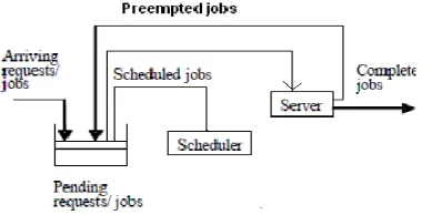
Multiprocessing is the use of two or more central processing units within a single computer system and refers to the ability of the system to support more than one processor and/or the ability to allocate tasks between them. The multiprocessor scheduling problem is identified to be Non-deterministic Polynomial (NP) complete except in some cases [1]. Figure (1) shows the representation of job scheduling in a multiprocessor. Here each request is a job or process [2]. A job scheduling policy uses the information associated with requests to decide which request should be serviced next. Waiting requests are kept in a pending request lists. Scheduler examines the pending requests and selects one for servicing at the time of performance. This request is handled over to server. A request leaves the server when it completes or when it is preempted by the scheduler, in which case it is put back into the list of pending requests. In either situation, scheduler performs scheduling to select the next request to be serviced. The scheduler records the information concerning each job in its data structure and maintains it all through the life of the request in the system.
Figure 1. A Schematic of Job scheduling in a multiprocessor
In a multiprocessor architecture, the job scheduling problem is partitioning the jobs between different processors by achieving minimum finishing and waiting times concurrently. If ‘n’ different jobs and ‘m’ different processors are considered, the search space is given by
(m × n)!
Size of search space =
(m!)n
Longest Processing Time (LPT), Shortest Processing Time (SPT) and traditional optimization algorithms were used for solving this type of scheduling problems [3], [1] & [4]. When all the jobs are in ready queue and their respective time slice is determined, LPT selects the longest job and SPT selects the shortest job, thereby having shortest waiting time. Thus SPT is minimizes the waiting time. The total finishing time is defined as the total time taken for the processor to complete its job and the waiting time is defined as the average of time that each job waits in ready queue. In manufacturing, makespan is defined as the time variation between the start and finish of a series of jobs or tasks.
integrated algorithm proposed by Song et al., 2010[6] for production scheduling. Sun et al., 2010[7] proposed genetic algorithm for the job shop problem. Most of the researches use PSO for job shop scheduling problem, like Xia et al., 2006 [8], Ge et al., 2005 [9] and Pan et al., 2007[10], etc.
II. OPTIMIZATION TECHNIQUES
There are several well known meta heuristics like Genetic Algorithm, Ant colony optimization and Tabu search has been applied to the earlier problem. In this paper, the hybrid algorithms based on the PSO and SA are studied and applied to the scheduling problems. The PSO as an evolutionary algorithm, it merges coarse global search capability and local search ability. SA as a neighborhood search algorithm, it has strong local search ability and can employ certain probability and can to avoid becoming trapped in a local optimum. The Hybrid Particle Swarm Optimization (HPSO) is a combination of three SA algorithms and PSO. In HPSO, PSO is used to find the particle’s each best solution and SA is used to find its best neighbor solution. So HPSO is a viable and effective approach for the job-shop scheduling problem.
Improved PSO (ImPSO) having better optimization result than PSO by splitting the cognitive component of the PSO into two different component. (i) Good experience component - the previously visited best position similar to the general PSO method. (ii) Bad experience component – a particle’s previously visited worst position.
A. Particle Swarm Optimization (PSO):
In 1995, Kennedy and Eberhart introduced PSO which had the fish or birds feeding style. PSO includes a particles’ population, each particle consists of a potential solution to the problem and a velocity [3]. Each particle moves around in the D dimensional space with the velocity and constantly adjusted velocity according to the experience of its own and its neighbors’.
a. The description of the PSO:
Xi = (xi,1, xi,2,..., xi,d) - the position of the ith particle
The concept of the PSO involves to update the velocity and position of each particle towards the best position of the D-dimensional space according to its best Position Pbesti
and the best particle of all gbest in each iteration, the equation is illustrates as Eqs.(1) and Eqs.(2).
vi,d(t+1)=w×vi,d(t)+c1×r1×(gbest(t)-xi,d(t))+c2×r2×
(pbesti,d(t)-x i,d(t)) (1)
xi,d (t+1) = xi, d(t) + vi,d(t+1) (2)
Here w is the inertia weight: constant in the interval [0, 1] c1 and c2 are learning rate: non-negative constants
r1 and r2 are random variable in the interval [0, 1]
vi,d∈ [vmax, vmax], The termination for iteration is determined
by the maximum generation or a designated value of the fitness.
B. Improved PSO (ImPSO):
To calculate the new velocity, the bad experience of the particle also taken into consideration [2]. On including the characteristics of Pbest and Pworst in the velocity updating process along with the difference between the present best particle and current particle respectively, the convergence towards the solution is found to be faster and an optimal solution is reached in comparison ith conventional PSO approaches. This infers that including the good experience and bad experience component in the velocity updating also reduces the time taken for convergence.
a. Algorithmic steps for ImPSO:
Step1: Select the number of particles, generations, tuning accelerating coefficients C1g, C1b, and C2 and random
numbers r1, r2 and r3 to start the optimal solution searching Step2: Initialize the particle position and velocity.
Step3: Select particles individual best value for each generation.
Step4: Select the particles global best value, i.e. particle near to the target among all the particles is obtained by comparing all the individual best values.
Step5: Select the particles individual worst value, i.e.
particle too away from the target.
Step6: Update particle individual best (pbest), global best (gbest), particle worst (Pworst) in the velocity equation (3) and obtain the new velocity.
vi = w×vi+C1g×r1(Pbesti-Si)×Pbesti+C1b×r2×(Si-Pworsti)×
Pworsti+C2×r3×(Gbesti-Si) (3)
Step7: Update new velocity value and obtain the position of the particle.
Step8: Find the optimal solution with minimum ISE by the
updated new velocity and position.
The ImPSO approach was applied to the multiprocessor scheduling problem. The good experience component and the bad experience component are included in the process of velocity updating and the finishing time and waiting time computed.
C. Simulated Annealing (SA):
In 1953, Metropolisin proposed SA algorithm. It starts from an initial solution‘s’, engenders a new solution S’ in the locality of the original solution S. The objective function’s change of value is calculated by, △=f(S’)–f(s). For a minimization problem, if △<0, the transition to the new solution is accepted. If △>0, the transition to the new solution is accepted with probability, usually denoted by the
function, exp (-△/T), where T is a control parameter
a. Structure of SA:
Design SA algorithms SA1, SA2 and SA3 by the use of different kinds of neighborhood structures, which are named Swap, Insert1, and Insert2, respectively. The description of SA1 as follows (SA2 and SA3 similar with SA1).
For Pbest of particle X(i)
Step1: Initialize T0, λ and L, Tk=T0, P=Pbest
Step2: computation while (Tk>Tend) i=1 while i<=L
Create a neighbor solution Pnew of P busing swap neighborhood structure Calculate the fitness of Pnew
If △=f(Pnew)-f(Pbest)<0 then Pbest=Pnew elseif(exp(-△/Tk)>random[0,1]) then P=Pnew endif i=i+1
Tend - termination temperature.
The performance of SA algorithm is influenced by the neighborhood. A large number of candidate solutions in rich neighborhood will increase the chance of finding good solutions; the computation time will also increase.
D. HPSO:
PSO algorithm is relevant to a given problem, so it is problem-independent and fitness costing for each solution. This makes PSO more robust than other search algorithms. By the use of PSO we cannot find the required optima. SA has strong local search ability. By designing the neighborhood structure we can avoid individuals being trapped in local optimum more efficiently. Thus, a hybrid of PSO and SA is proposed and named as Hybrid PSO (HPSO) for Job Shop Problem [14].
a. Description of HPSO:
Step 1: Initialize
a) Initialize the parameters such pop, Itermax, wmax, wmin,
c1max, c1min, c2, initialize the selection probability ρ1,ρ2 and ρ3 of three SA algorithms.
b) Initialize particles and velocities in the D-dimensional problem space.
c) Evaluate the fitness of each particle in the population, record the best particle as gbest of swarm and record the local best solution Pbest respectively.
Step2: Computation Iter = 1
while Iter < Itermax
j=1
While j≤ pop
Update the velocity and position of the particle X j (Iter1+1) according to Eqs.(1) and (2) respectively.
Evaluation fitness of Xj (Iter+1),
If f (Xj(Iter+1) > f (pbestj) then
pbestj = Xj(Iter+1) and randomly select one of the three SA
and execute it on Pbest.
endif
If (f(pbestj)>f(gbest)), then gbest=Xj(Iter+1)
endif j=j+1 wend Iter = Iter+1
Step3: Determine. If the solution of gbest do not achieve the target, the select a SA algorithm and update the parameter and execute it on gbest of swarm,
Step4: Output the sufficiently good fitness value or a
specified number of generations.
E. Hybrid Improved PSO (Hybrid ImPSO):
The ImPSO algorithm is problem independent so they gained results can be further improved with the SA. The probability of getting trapped in a local minimum can be SA and called as Hybrid Improved Particle Swarm Optimization Hybrid ImPSO [7].
a. Steps involved in Hybrid ImPSO:
Step1: Initialize temperature T to a particular value.
Step2: Initialize the number of particles n and its value may be generated randomly. Initialize swarm with random positions and velocities.
Step3: Compute the finishing time for each and every
particle using the objective function and also find the “pbest“
i.e., If current fitness of particle is better than “pbest” the set “pbest” to current value.
If “pbest” is better than “gbest then set “gbest” to current particle fitness value.
Step4: Select particles individual “pworst” value i.e.,
particle moving away from the solution point.
Step5: Update velocity and position of particle as per
equation (3).
Step6: If best particle is not changed over a period of time, find a new particle using temperature.
Step7: Accept the new particle as best with probability as exp-(ΔE/T). ΔE is the difference between current best particles fitness and fitness of the new particle.
Step8: Reduce the temperature T.
Step 9: Terminate the process if maximum number of
iterations reached or optimal value is obtained, else go to step 3.
III. RESULTS AND DISCUSSION
The instances designed by Lawrence (1984) are taken form web ftp://mscmga.ms.ic.ac.uk/pub/jobsgop1.txt. Results are compared with some existing literature works [15], [16] and [17]. The 1.86 GHz Pentium 4 desktop computer with 512 MB RAM was used to do this work.
(TSA), An effective PSO and AIS-based Hybrid Intelligent algorithm (HIA) and Filter-and-Fan (F&F) approach.
Table 1. Benchmark Instances’ Results
Inst ance
Size
(n,m) C* HPSO TSA HIA F&F
LA1 10,10 945 946 945 945 945
LA2 10,10 845 848 845 845 850
LA3 20,10 1216 1225 1216 1216 1225
LA4 20,10 1152 1168 1160 1168 1170
LA5 15,15 1268 1279 1268 1268 1276
LA6 15,15 1397 1423 1407 1411 1418
LA7 15,15 1222 1236 1229 1233 1228
Figure (2) shows the comparison chart of instances with the values of the best solutions for the various algorithms. This chart concludes that, HPSO can yields best solution and solves the job scheduling problems efficiently, because of the combination of SA which is used to increase the local search ability and speedup the convergence rate of PSO.
Figure 2. Chart for Instances’ Best Solutions
The PSO, ImPSO and Hybrid ImPSO algorithms were applied to the same set of processors with the assigned number of jobs, as done in case of genetic algorithm (GA). The number of particles are100, number of generations are
250, the values of c1=c2=1.5 and ω=0.5. Hybrid ImPSO
algorithm is applied to the multiprocessor scheduling algorithm and the temperature T as 5000. The Intel Pentium 2 core processors with 1GB RAM were used to do this work.
Table (2) shows the completed finishing time of the relevant number of processors and jobs exploiting PSO, ImPSO and Hybrid ImPSO. The ImPSO has been reduced in association with GA and PSO, because of bad experience and good experience component in the velocity updating process. In case of Hybrid ImPSO, there is a severe decline in the finishing time, because combining the effects of the SA and ImPSO; finally better solutions have been achieved.
Table 2. Finishing Time for Job Scheduling
Figure (3) shows the difference in finishing time for the assigned number of jobs and processors using PSO, ImPSO and Hybrid ImPSO. It is observed, that the Hybrid ImPSO
had variation in finishing time for the assigned number of jobs and processors.
Figure 3. Finishing time for jobs in multiprocessor
Table (3) shows the completed waiting time of the appropriate number of processors and jobs exploiting with PSO, ImPSO and Hybrid ImPSO. The Hybrid ImPSO is a drastic reduction in the waiting time while compared with PSO and ImPSO. Finally better solutions have been achieved in Hybrid ImPSO.
Table 3. Waiting Time for Job Scheduling
Processors 2 3 3 4 5
No.of jobs 20 20 40 30 45 PSO 30.1 45.92 42.1 30.7 34.91
Imp PSO 29.12 45 41 29.7 33.65
Hybrid Imp PSO 25.61 40.91 38.45 26.5 30.12
Figure (4) shows the variation in waiting time for the allocated number of jobs and processors using PSO, ImPSO and Hybrid ImPSO. It is concluded that the Hybrid ImPSO had discrepancy in waiting time for the assigned number of jobs and processors.
Figure 4. Waiting time for jobs in multiprocessor
IV. CONCLUSION & FUTURE WORK
This paper deals with the PSO, HPSO, ImPSO and Hybrid ImPSO algorithms which are useful to solve the job shop scheduling problems and reduces the finishing and waiting time of the multiprocessors. In HPSO algorithm, PSO may fail to locate optima, then SA employs certain prospects, but the serial execution made is less competent. So PSO and SA were combined and the approach yields good solution than other algorithms. The greater results specify the merging of PSO and SA. ImPSO algorithm is used for finding good and bad experience component in the velocity renews and shrink the time taken for convergence. In multiprocessor job shop scheduling, Hybrid ImPSO is applied to partition the tasks in the processors by conquering
Processors 2 3 3 4 5 No.of jobs 20 20 40 30 45
PSO 60.52 56.49 70 72.2 70.09
Imp PSO 57.34 54.01 69 71 69.04
minimum finishing, waiting time and quick processing time. Finally, Hybrid ImPSO algorithm has attained better results. Depending upon literature survey, no one worked with optimal scheduling algorithms in distributed data warehouse. Future work can be done for new optimal scheduling algorithm that will give fruitful result to reduce the number of executors and runtime in distributed data warehouse.
V. ACKNOWLEDGEMENT
I thank the Karpagam University and my guide Dr.M.Hemalatha for the Motivation and Encouragement to make this research work as successful one.
VI. REFERENCES
[1] Gur Mosheiov and Uri Yovel, “Comments on Flow-Shop and Open-Shop Scheduling with a Critical Machine and Two Operations Per Job,” European Journal of Operational Research (Elsevier), 2004.
[2] K. Thanushkodi and K.Deeba, “A Comparative Study of Proposed Improved PSO Algorithm with Proposed Hybrid Algorithm for Multiprocessor Job Scheduling,” International Journal of Computer Science and Information Security, vol. 9(6), 2011, pp. 221-228.
[3] Ali Allahverdi, C.T. Ng, T.C.E. Cheng, Y. Mikhail and Y. Kovalyov, “Survey of Scheduling Problems with Setup Times or Costs,” European Journal of Operational Research ( Elsevier), 2006.
[4] Gur Mosheiov and Daniel Oron, “Open-Shop Batch Scheduling with Identical Jobs,” European Journal of Operations Research (Elsevier), 2006.
[5] Lei Wang and Wenqi Huang, “A New Neighborhood Search Algorithm for Job-Shop Scheduling Problem,” Computer Journal, vol. 28(5), 2005, pp. 809-815.
[6] Song Cunli, Liu Xiaobing, Wang Wei and Huang Ming, “Dynamic Integrated Algorithm for Production Scheduling Based on Iterative Search,” Journal of Convergence Information Technology, vol. 5(10), 2010, pp. 159-166. [7] Sun Liang, Cheng Xiaochun and Liang Yanchun,”Solving
Job-Shop Scheduling Problem using Genetic Algorithm with Penalty Functions,” Journal of Next Generation Information Technology, vol. 1(1), 2010, pp. 65-77.
[8] Xia Wenjun and Wu Zhiming, “A Hybrid Particle Swarm Optimization Approach for the Job-Shop Scheduling Problem,” Internal Journal Advanced Manufacture Technology, vol. 29(1), 2006, pp. 360-366.
[9] Ge Hongwei and Liang Yanchun, “A Particle Swarm Optimization-Based Algorithm for Job-Shop Scheduling Problem,” Journal of Computational Method, vol. 2(1), 2005, pp. 419-430.
[10] Quanke Pan, Wang Hongwen, Zhu Jianying and Zhao Baohua, “A Hybrid Scheduling Algorithm Based on Particle Swarm Optimization and Variable Neighborhood
Search,” Chinese journal of Computer Integrated Manufacturing System, vol. 13(1), 2007, pp. 323-328. [11] W. Bozejko, J. Pempera and C. Smuntnicki, “Parallel
Simulated Annealing for the Job-Shop Scheduling Problem, Lecture notes in Computer Science,” Proceedings of 9th International Conference on Computational Science, vol. 5544, 2009, pp. 631-640.
[12] H.W. Ge, W. Du and F. Qian, “A Hybrid Algorithm Based on Particle Swarm Optimization and Simulated Annealing for Job-Shop Scheduling,” Proceedings of 3rd International Conference on Natural Computation, vol. 3, 2007, pp. 715– 719.
[13] Weijun Xia and Zhiming Wu, “An Effective Hybrid Optimization Approach for Multi-Objective Flexible Job-Shop Scheduling Problems,” Journal of Computers & Industrial Engineering, vol. 48(2), 2005, pp. 409-425.
[14] Song Cunli, Liu Xiaobing, Wang Wei, Bai Xin, A Hybrid Particle Swarm Optimization Algorithm for Job-Shop Scheduling Problem, International Journal of Advancements in Computing Technology, 3(4), 2011, 79-88.
[15] Pezzella Ferdinando and Merelli Emanuela, “A Tabu Search Method Guided by Shifting Bottleneck for Job-Shop Scheduling Problem,” European Journal of Operational Research, vol. 120(2), 2000, pp. 297-310.
[16] Ge Hongwei, Sun Liang, Liang Yanchun and Qian Feng, “An Effective PSO and AIS Based Hybrid Intelligent Algorithm for Job-Shop Scheduling,” IEEE Transactions on systems, Man, and Cybernetics-Part A: Systems and Humans, vol. 38(2), 2008, pp. 358-368.
[17] Rego César and Duarte Renato, “A Filter-and-Fan Approach to the Job-Shop Scheduling Problem,” European Journal of Operational Research, vol. 194(3), 2009, pp. 650-662.
Short Bio Data for the Author
S.Krishnaveni completed MCA, M.Phil., and currently pursuing Ph.D. in computer science at Karpagam University under the guidance of Dr.M.Hemalatha, Head, Dept. of Software System and Research, Karpagam University, Coimbatore. Published four papers in International Journals and also presented one paper in International Conference. Area of Research is Data Mining and Data Warehousing.