Sample Size Calculations for Crossover Thorough
QT Studies: Non-inferiority and Assay Sensitivity
Suraj P. Anand,1,∗ Sharon C. Murray,2 and Gary G. Koch3
1Department of Statistics, North Carolina State University, Raleigh,
North Carolina, USA
2Discovery Biometrics, Oncology, GlaxoSmithKline, Research
Triangle Park, North Carolina, USA
3Department of Biostatistics, University of North Carolina at Chapel Hill,
Chapel Hill, North Carolina, USA
Institute of Statistics Mimeo Series #2621
Abstract
The cost involved in running a ‘thorough QT/QTc study’ is substantial and an adverse outcome of the study can be detrimental to the safety profile of the drug, hence sample size calculations play a very important role in ensuring an adequately powered thorough QT study. Current literature offers some help in designing such studies but these methods are limited and mostly apply only in the context of linear mixed models with compound symmetry covariance structure. It is not evident that such models can satisfactorily be em-ployed to represent all kinds of QTc data, and the existing literature inadequately addresses if there is a change in sample size and power, in case one looks to more general covariance structures for the linear mixed models. We assess the use of some of the existing methods to design a thorough QT study, based on data arising from a GlaxoSmithKline (GSK) con-ducted thorough QT study, and explore newer models for sample size calculation. We also provide a new method to calculate the sample size required to detect assay sensitivity with a high power.
Keywords: Correlation structure; ICH E14; Monte Carlo simulation; Power and Sample size; QTc prolongation; thorough QT/QTc study
1
Introduction
Thorough QT studies are becoming a necessary part of the clinical profile of existing and investigational new drugs. The International Conference of Harmonization (ICH) E14 guidelines (available atwww.fda.gov/cder/guidance/) mandate conducting a thorough QT study on any non-antiarrythmic drug to determine whether the drug has a threshold pharmacological effect on cardiac repolarization, as detected by QTc prolongation, before it can be approved and marketed. The cost involved in running a thorough QT study is substantial and an adverse outcome of the study can be detrimental to the safety profile of the drug, hence sample size calculations play a very important role in ensuring a small but adequately powered thorough QT study.
The ICH E14 guidance document describes in detail the scope, conduct and implications of a thorough QT study. Recent developments in the area of analysis of a thorough QT study include articles by Eaton et al. (2006), Boos et al. (2007) and Anand and Ghosh (2009), though the standard way of analyzing QT data still remains to be the intersection-union-based test that compares the two-sided 90% upper confidence interval for the time-mached mean difference between drug and placebo at each time point with the regulatory threshold of 10 msec. A review of statistical design and analysis in thorough QT studies can be found in Patterson et al., 2005.
Measurements taken in a QT study are naturally in time order and hence multivariate methods are the most appropriate tools for analyzing such a data. Current literature offers some help in designing such studies but these methods are limited and apply only in the context of linear mixed models with rather restrictive assumptions on the covariance structure. Hosmane and Locke (2005) performed a simulation study to assess the impact of sample size on power for fixed covariance parameters, estimated from their own data, for a four-period crossover study. They used a multivariate model for the data and their results indicate that power may depend on the covariance structure and the components of the mean difference vector between drug and placebo. Recently, the Journal of Biopharmaceutical Statistics issued a special edition with a wide range of articles on statistical issues in design and analysis of thorough QT studies (Volume 18, Issue 3, 2008), some of which address the sample size calculations in commonly encountered settings.
et al. (2008) assess the impact of the number of replicate measurements on sample size for linear mixed models. It is not known whether such models will fit all data from QT studies well and if there is a change in sample size and power, in case one looks beyond the commonly employed linear mixed models. We address the robustness of sample size and power calculations to departures from the linear mixed models by considering a compound symmetry correlation structure with a random period effect, a mixed model with variable correlation across time points, and a completely unstructured covariance matrix for the time-matched mean difference vector.
Another important aspect of a thorough QT study is the assay sensitivity of the trial. Zhang and Machado (2008) point out that the trial must be able to detect obvious differences, as indi-cated by a ‘positive’ result for the positive control. Zhang (2008) provides a local test using the Bonferoni adjustment for multiplicity, as well as a global test using the averaged time-matched mean difference that does not require a multiplicity correction. Both these tests provide reason-able methods for assessing assay sensitivity but they have their advantages and disadvantages. Tsong et al. (2008) provides a discussion on these two approaches for assessing assay sensitivity. We propose a slightly different approach that is less stringent than the Bonferoni correction and does not have the risk involved with the global test.
In Section 2, we present a motivating example and review the existing literature for sample size calculations. In Section 3, we provide a few plausible models for the QT data for crossover studies that extend the usual linear mixed models to a more general mixed model representation, and can be used to calculate power and sample size in more general settings. More specifically, we provide a methodology to calculate sample sizes for a design that accounts for variable correlation between the time points within any period. We provide a new method to calculate the minimum sample size required to detect assay sensitivity with a high power in Section 4. In Section 5, we use the example dataset to illustrate our methods and in Section 6 we present the conclusions and a discussion. We also provide sample size tables in the Appendix for a variety of crossover settings for the linear mixed effect model with and without a random period effect and they can be used by practitioners to design a crossover thorough QT study.
2
A Motivating Example
doses of the new drug. Subjects were randomized to one of the four sequences defined with a William’s square design (Senn, S. J., 2002), with a washout period of at least 14 days between treatments. During each period, subjects received the assigned treatment for 5 days and ECG readings were taken in triplicate at each time point for a full day prior to dosing and on the fifth day of dosing. Times on the baseline day were matched to the time points for the fifth day of the dosing period. Change from baseline values were calculated by subtracting the time-matched averaged baseline value from the average of the triplicate readings on the fifth day of dosing. The nine time points in hours (hr) used in this study were predose, 0.5 hr, 1 hr, 2 hr, 3 hr, 4 hr, 6 hr, 12 hr, and 23.25 hr. Several different corrections for QT interval were actually done in the study, but the outcome of interest that we will focus on here is Fridericia’s corrected QT interval (QTcF). Sample size was planned to ensure that 40 subjects would complete the study with evaluable ECG readings. The achieved sample size was slightly larger.
Suppose we use a mixed effect model for the change from baseline QTcF values, with base-line value, sequence, period, treatment, time, and a treatment by time interaction term as fixed effects, and subject as the random effect. This model inherently assumes that the co-variance structure for the vector of baseline corrected QTcF measurements is compound sym-metric; a mixed model analysis resulted in the between subject variability estimate σs = 13 and the intra-subject correlation ρ = 0.8. The mean difference vector between the baseline corrected QTcF values for the supratherapeutic dose and placebo for this thorough QT study was (−1.64,−1.02,2.29,1.86,0.79,0.1,1.95,0.17,0.03).
Suppose that we are planning to run a similar crossover study with ten time points and a full day of baseline measurements prior to dosing, and we wish to power against an alternative hypothesis with a hill structure, such that QTcF initially increases over time and then decreases after reaching the maximum, and θ= 3 msec. Using the sample size estimates under indepen-dence given in Table 10 by Zhang and Machado (2008) one would require over 87 subjects to declare a thorough QT study successfully negative with 85% power. But this is a very conser-vative sample size estimate as it ignores the correlation between the time points and assumes a constant time-matched mean structure which may not be the case. The sample size required if we do not assume independence cannot be obtained in a straightforward manner and requires simulations. Zhang and Machado (2008) present some sample size estimates using simulations for a hill mean structure and a compound symmetry covariance structure with ρ = 0.5 for various values of σs, but these results are presented for θ= 5 msec and hence cannot be used to design our study.
the time points within any period given that the time points pertaining to the measurements taken on the same subject are not equispaced. For example, it is likely that the measurements taken within the first six hours are more correlated than those taken after that. It is of interest to assess the impact of the covariance structure on the planned sample size for the new study.
The time-matched mean difference vector between the baseline corrected QTcF values for the positive control moxifloxacin and placebo was (0.69,5.05,9.85,10.63,11.16,11.64,8.07,6.71,5.25). To ensure trial sensitivity of the new study, the sample size also needs to be large enough to have a high power to detect a positive QT effect for the positive control.
3
A Multivariate Framework for Crossover Design
In this section, we provide a framework for crossover designs that can be used to conduct simulations to compute the power and sample size for a thorough QT study with varying assumptions about the structure of the variance-covariance matrix. In a crossover design, subjects receive sequences of treatments (some (incomplete block) or all (complete block) of the study treatments) with the objective of studying differences between individual treatments (or sub-sequences of treatments) (Senn, S. J., 2002). Each individual in such a design serves as his own control and hence a crossover design requires a smaller sample size to achieve the same precision of the estimates than a parallel design. A 2x2 cross-over design refers to two treatments and two sequences (treatment orderings). For example, if the two treatments are placebo and drug then one sequence receives placebo in the first period followed by drug in the second period. The other sequence receives drug and placebo in a reverse ordering. The design includes a washout period between the two treatment periods to remove any carry-over effects. In an actual thorough QT study, subjects would actually receive multiple treatments, including placebo, active control, and 2 or 3 drug arms. We will calculate sample size based on a single comparison of drug to placebo and then apply that sample size to the full study.
LetY1i andY2i, i= 1, . . . ndenote the vectors of p baseline corrected QTc measurements taken on subjection the placebo and drug arms respectively, wherendenotes the total number of subjects in the study, and p is the total number of time points. The measurements for each treatment are assumed to be distributed identically and independently (iid), arising from correspondingp-variate normal distributions. However,Y1andY2are not independent because these are observations taken on the same individuals. In matrix notation, this can be represented as follows:
Y1i
Y2i
!
∼ N2p
µ1
µ2
!
, Σ11 Σ12
Σ21 Σ22 !!
where µ1 and µ2 are the population means for placebo and drug respectively, the covariance sub-matricesΣ11andΣ22represent the covariance structures for the data vectors corresponding to subjects in the placebo and the drug arms respectively, covariance sub-matricesΣ12=Σ
′ 21 represent the covariances between data vectors corresponding to the same subject in period 1 and period 2 respectively. All the covariance sub-matrices are assumed to be completely known, either on the basis of previous studies or a large sample size for the current study. The parameter of interest is the vector of the time-matched population mean differences between drug and placebo ∆ =µ1 −µ2. Analogous to a univariate paired sample test, this problem can be reduced to a multivariate paired one sample setup. If we denote by Di the difference between the subject matched data vectors forith subject Di =Y2i−Y1i, then
Di iid∼ Np(∆,Σdif f), i= 1, . . . , n (2)
whereΣdif f =Σ11+Σ22−Σ12−Σ ′
12is the completely known covariance structure for the differ-ence. Now if we denote the sample time-matched mean difference by d,d=P
i(y2i−y1i)/n, then
d∼ Np(∆,Σd), (3)
whereΣd=Σdif f/n.
Each individual component ofd follows a univariate normal distribution.
dk∼ N1(∆(k), σd(kk)), k= 1, . . . p, (4)
whereσd(kk)is thekth diagonal element of the covariance matrixΣd. Thus we can sample from the distribution of d and construct confidence intervals on the individual components of ∆k. A 95% one sided upper confidence limit for ∆k, k=1,. . . p, is given bydk+z0.05√σd(kk), where z0.05= 1.645 is the 95th quantile of the standard normal distribution. Redefining the standard test in terms of confidence intervals, we can set the power equation to be
power =P{max
3.1 A Simple Linear Mixed Effect Model
We start by adopting the widely used linear mixed effect model for the crossover data, which can be written succinctly in a matrix notation for theith subject as
Y1i
Y2i
!
=Yi=Xiβ+Ziγi+ǫi, i= 1, . . . , n, (6)
whereXiβ denotes the fixed effect part of the model with treatment, time, treatment by time interaction, period baseline QTc, period and sequence as the fixed effects, and Ziγi denotes the random effect part of the model, with random subject effect and random period in subject effect as the random components. The actual model may have more study specific covariates. The benefit of using a random period effect is that it allows for the correlation between two observations from the same period (ρ1) to differ from correlations between two observations from
different periods (ρ2). We assume that ǫi ∼ N2p(0, σe2I2p), γi ∼ N3
0 ,
σ2s 0 0 0 σ2p 0 0 0 σ2
p
with all random effect components independent of each other. With Zi=
1p 1p 0p
1p 0p 1p !
,
V ar(Yi) =ZiV ar(γi)Z′i+σe2I2p =
(σ2s+σ2p)Jp+σe2Ip σ2sJp
σs2Jp (σs2+σp2)Jp+σ2eIp !
.
If we letσ2 =σ2
s +σp2+σe2,ρ1= (σs2+σp2)/σ2, and ρ2=σs2/σ2, then
V ar(Yi) = σ
2{(1−ρ
1)Ip+ρ1Jp} ρ2σ2Jp
ρ2σ2Jp σ2{(1−ρ1)Ip+ρ1Jp} !
,
whereJp =1p1 ′
p. Using the above results, we can calculate the variance of Di as
V ar(Di) = Σdif f =−I I
V ar(Yi) −I
I
!
= 2σ2{(1−ρ1)Ip+ (ρ1−ρ2)1p1 ′
p}, (7)
and use it for the calculation of sample size and power as outlined above.
A special case of this model is one with a fixed period effect (σp = 0) as utilized by Zhang and Machado (2008), where all the observations taken on any subject follow a simple compound symmetry covariance model regardless of the period to which they belong, with the overall variability σ=p
(σ2
Boos et al. (2007) showed that the variance for the difference in this linear mixed model with a random period effect can be represented in a compound symmetric form. The above model assumes a compound symmetric covariance structure for the observations taken in any one period. Such an assumption may not be appropriate given that the time points pertaining to the measurements taken on the same subject are not equispaced. For example, it is likely that the measurements taken within the first six hours are more correlated than those taken after that. We next propose a model to account for such a phenomenon.
3.2 A Mixed Model to Account for Variable Correlation Across Time Points
On lines similar to the above set up, we add one additional random component for timeband×period effect with its contribution to the overall variability denoted by σtb. Timeband is an indicator variable with two classes, with observations for the time points close together clubbed in one class and the remaining observations in the other class. This is equivalent to assuming that the observations taken on the firstltime pointsl < p in any period are more correlated than those taken after that. In addition, observations taken in the same period are more correlated than those taken in different periods. If we let σ2 =σ2
s+σtb2 +σp2+σe2, ρ11 = (σs2+σtb2 +σp2)/σ2, ρ12= (σs2+σp2)/σ2, and ρ2 =σs2/σ2, then the variance ofYi is given by V ar(Yi) =
σ2
(1−ρ11)Il+ρ11Jl ρ12Jl×(p−l) ρ12J(p−l)×l (1−ρ12)Ip−l+ρ12Jp−l
!
ρ2Jp
ρ2Jp
(1−ρ11)Il+ρ11Jl ρ12Jl×(p−l) ρ12J(p−l)×l (1−ρ12)Ip−l+ρ12Jp−l
!
,
whereJr×s=1r1 ′ s.
Doing similar algebra as in the previous subsection, we obtain
V ar(Di) = 2σ2 (1−ρ11)Il+ (ρ11−ρ2)Jl (ρ12−ρ2)Jl×(p−l) (ρ12−ρ2)J(p−l)×l (1−ρ12)Ip−l+ (ρ12−ρ2)Jp−l
!
, (8)
3.3 A Mixed Model With Completely Unstructured Covariance Matrix for the Difference
There is no evidence that any particular covariance structure fits QT data well. Even the existing literature does not favor any one model to represent the QT data. A compound symmetric model is usually invoked for the sake of simplicity. An unstructured covariance matrix for V ar(Yi) involves a large number of parameters. For example, if ten time points are used in a 2-way crossover study, then the completely unstructured design yields 2p(2p+ 1)/2 = 210 covariance parameters. An alternative is to allow a completely unstructured covariance matrix for the difference vector, i.e., V ar(Di) = Σdif f = ((σkk′)), whereσkk′ is the covariance between any two time points k and k′. For a 2-way crossover study with ten time points, V ar(Di) will have p(p+ 1)/2 = 55 covariance parameters. Given an estimate for V ar(Di), sample size and power can be calculated as outlined above.
4
Sample Size Assessment for Assay Sensitivity
According to the ICH E14 guidelines, any thorough QT study should include a positive control to assess the assay sensitivity. The positive control should demonstrate a mean QT effect in excess of the regulatory threshold of 5msec. This gives reasonable assurance that the trial is sensitive enough to detect such an effect of the study drug. The hypotheses of interest can be set based on a testing procedure as outlined in Zhang and Machado (2008) as follows:
H0 : q \
k=1
{µ2(k)−µ1(k)} ≤5
H1 : q [
k=1
{µ2(k)−µ1(k)}>5
(9)
advantage of this approach is to reduce the extent for adjusting for multiplicity for a large number of time points. Zhang and Machado (2008) indicate a few references that provide methods to account for multiplicity in a general setting.
Zhang (2008) provides a local method using the Bonferoni adjustment for multiplicity, as well as a global method using the averaged time-matched mean difference that does not require a multiplicity correction. The paper also provides sample size calculations based on these methods. While both of these methods are reasonable methods for assessing assay sensitivity, the local test may be too stringent if the number of pre-specified time points is too large. On the other hand, the main risk with the global test is that the average time-matched mean difference may have dilution due to some time points with small differences even though there is a large difference at some time point. Tsong et al. (2008) provides a discussion on these two approaches for assessing assay sensitivity.
We take a somewhat different approach that is less stringent than the Bonferoni correction and does not suffer from the risk involved with the global test as proposed in Zhang (2008). More specifically, we use the Hailperin-Ruger method to assess for significance at a subset of the total number of time points. This approach was described by Abt (1991) for partially global hypotheses in the context of multiplicity problems in clinical trials.
For the assessment of assay sensitivity with the Hailperin-Ruger method, the global null hypothesis in (9) for the q pre-specified time points has contradiction with one-sided type I error when a pre-specified minimum numberq′ ≤q of the individual hypotheses within (9) for the respective time points have contradiction at the adjusted α∗ = q′
qα one-sided significance level. These q′
hypotheses, with each to have contradiction at the α∗ significance level, may
appear anywhere within the ‘Hailperin-Ruger area’ defined by the null hypothesis in (9), and the basis for their contradiction can be throughq′ of the corresponding two-sided 100(1-2α∗)%
confidence intervals having their lower bounds exceed 5 msec. A proof of how the Hailperin-Ruger method maintains type I error at one-sided α for the assessment pertaining to (9) is provided in the Appendix.
To obtain sample size for a given power, one can use a superiority test for a crossover design, based on a two-sample t-test with level α∗ and a superiority margin of 5 using any standard
5
Application to the Real Dataset
We revisit the example given in Section 2. This GSK conducted thorough QTc study was a crossover trial with 4 treatment arms, with QTcF measurements taken at nine time points in each period. The model used to analyze the data was as described in Section 3.1 (Equation (6)) withYi as a 4p×1 vector of change from baseline QTcF values from each of the 4 periods. Fixed effects included baseline value, sequence, period, treatment, time, and a treatment by time interaction term. This model inherently assumes that the data structure for the vector
Yi is compound symmetric with a given total variance σ2 = σ2s +σe2 and ρ = σs2/σ2 as shown in Section 3.1. Since period is treated as a fixed effect, σ2p = 0. In this case, the individual components of the vector of differences can be easily shown to be independent with
Σdif f = 2σe2I.
The covariance parameters obtained from this analysis were σ2 = 209.2, σ2s = 168.5, and σe2 = 40.7, so thatσ = 14.5 andσe= 6.4. This corresponds to the vector of change from baseline QTcF data,Yi, having compound symmetric structure withσ= 14.5 andρ = 0.806. The mean difference vector between the baseline corrected QTcF values for the supratherapeutic dose and placebo was (−1.64,−1.02,2.29,1.86,0.79,0.1,1.95,0.17,0.03) and hence a hill mean structure seems to be a suitable description for the mean difference vector.
Suppose that we are planning to conduct a similar crossover study with nine time points and a full day of baseline measurements prior to dosing, and we wish to power against an alternative hypothesis withθ= 3 msec. We compute sample sizes for three mean structures corresponding to this θ value. The three mean structures (Constant, Hill and Steady state) that we have used for the simulations are the most plausible ones. In the Constant mean model, the baseline corrected QTc is expected to remain constant across the time points. In the Hill mean model, the baseline corrected QTc is expected to initially increase and then decrease after reaching the maximum, whereas, in the Steady state mean model, it is expected to increase initially and then stabilize after reaching the maximum. We performed simulations based on the methods described in Section 3, using the formula for V ar(Di) provided in Section 3.1 (eq. (7)), with σ2 = 209.2 and ρ
1 =ρ2 = 0.806 to obtain the required sample sizes for 90% power. The first block of Table 1 summarizes these results.
It is clear from the results that the hill and the steady state mean models have a substantially lower sample size than the constant mean model; the sample sizes for the hill mean model are similar to those for the steady state mean model.
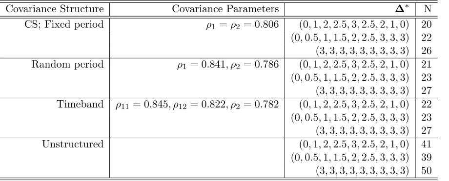
Table 1: Sample size calculations for the crossover design for 90% power for θ= 3 for various covariance structures
Covariance Structure Covariance Parameters ∆∗ N
CS; Fixed period ρ1=ρ2 = 0.806 (0,1,2,2.5,3,2.5,2,1,0) 20 (0,0.5,1,1.5,2,2.5,3,3,3) 22 (3,3,3,3,3,3,3,3,3) 26 Random period ρ1 = 0.841, ρ2 = 0.786 (0,1,2,2.5,3,2.5,2,1,0) 21 (0,0.5,1,1.5,2,2.5,3,3,3) 23 (3,3,3,3,3,3,3,3,3) 27 Timeband ρ11= 0.845, ρ12= 0.822, ρ2 = 0.782 (0,1,2,2.5,3,2.5,2,1,0) 22 (0,0.5,1,1.5,2,2.5,3,3,3) 23 (3,3,3,3,3,3,3,3,3) 27 Unstructured (0,1,2,2.5,3,2.5,2,1,0) 41 (0,0.5,1,1.5,2,2.5,3,3,3) 39 (3,3,3,3,3,3,3,3,3) 50
* Results for hill, steady state, and constant mean structures.
0.841 and 0.786 respectively. The sample size results from simulations based on the methods described in Section 3, using the formula for V ar(Di) provided in Section 3.1 (eq. (8)), with σ = 14.3,ρ1= 0.841 and ρ2 = 0.786 for the three mean structures are presented in the second block of Table 1. As with the earlier model, the sample sizes for the hill mean model are similar to those for the steady state mean model; the hill mean model and the steady state mean model have a substantially lower sample size than the constant mean model. It can also be seen that adding the random period effect to the model increases the sample size by only one in each case.
Next, we analyzed the data with an additional random component for timeband, so as to make observations taken during the first six hours in any period more correlated than those taken after that. The resulting covariance parameters obtained from this analysis were σ2 = 202.39,σ2
model.
Finally, we allowed for a completely unstructured covariance structure for the data for the time-matched mean difference vector between drug and placebo. This is the most general model and can be invoked if one is not comfortable making any assumptions about the covari-ance structure for the original data. This model can also be tried to assess the sensitivity of the sample sizes to the covariance assumption. One should note, however, that a totally unstruc-tured covariance structure might lead to a substantial loss of power because of the large number of parameters that need to be estimated. So, such a structure would be of some value only if the estimated unstructured covariance matrix was derived from a large study resulting in pre-cise covariance parameter estimates. The sample size results for this model for the GSK data, from simulations based on the methods described in Section 3, using the formula for V ar(Di) provided in Section 3.3, are presented in the last block of Table 1. As expected, the sample size required to achieve 90% power is substantially high with the unstructured covariance structure.
All the analyses and simulations were performed using SAS, version 8. The sample size results were based on 1000 simulation runs since the corresponding span of a two-sided 95% confidence interval about 90% power is about 2∗100p
(.9)(.1)/1000 ≈ 2%. Any sample size thus calculated for a 90% nominal power is expected to have the actual power in the range of 88%-92%. It is evident from the above analysis that there isn’t much change in power and sample size with a departure from the linear mixed model with a compound symmetric covariance structure unless one is confident about invoking a completely unstructured covariance matrix based on estimates from a large study. So, the commonly invoked compound symmetric covariance structure with fixed period effect or a linear mixed effect model with random period effect seems adequate. We provide some sample size results for these two popular models, for a variety of plausible parameter settings in the Appendix. We have given sample sizes under various mean and covariance structure parameter settings for a crossover design with ten time points, with fixed/random period effect. For the simplest model with a compound symmetry covariance structure for the data, we have provided results for two different parameterizations, one using variability estimates of the covariance parameters, and the other using the overall variability estimate and intra-subject correlation, so that depending on what information is available, one may use one or the other. These results are based on simulations similar to the ones described above and can be of great use for practicing statisticians in designing thorough QT studies for crossover designs. The details for these simulation results can be found in Anand, Murray and Koch (2008).
To assess the sample size required for trial sensitivity, we used a superiority test for a crossover design, based on a two-samplet-test with levelα∗, with a superiority margin of 5 msec,
a random period effect as an estimate of the within subject variability (σw =qσ2
p+σ2e = 6.6). The time-matched mean difference vector between the baseline corrected QTcF values for the positive control moxifloxacin and placebo was (0.69,5.05,9.85,10.63,11.16,11.64,8.07,6.71,5.25). So, we used a value of 11.5 msec in the alternative space for the calculations. It is easy to see from the time-matched mean difference vector that the time points 2 hr, 3 hr, 4 hr, and 6 hr appear to have a higher chance of yielding differences greater that 5 msec, so we selected these time points for our partial null with q = 4. We chose q′ = 2, with one-sided α = 0.05 that yields α∗ = 0.025 for our calculations. We used the sample size software PASS for our
calculations. A sample size of 24 achieves 90% power to detect assay sensitivity, based on a superiority test using a one-sided t-test with a superiority margin of 5 msec. One would then choose the maximum of the two sample sizes computed above, one for the study drug safety and the other for sensitivity analysis, as the final sample size for the study. Assuming a hill or a steady state mean structure for the vector of the time-matched mean differences, a sample size of 24 subjects will result into a study that is adequately powered to show non-inferiority as well as establish the sensitivity of the trial based on the example data. We see that assay sensitivity drives the sample size for this study.
6
Conclusions and Discussion
Multivariate methods are the most appropriate tools for analyzing data from a thorough QT study. Zhang and Machado (2008) provide a sample size formula assuming independence be-tween time points for a constant time-matched mean difference vector and they also present some simulation-based sample size estimates under the compound symmetry covariance struc-ture for a hill-type time-matched mean vector. Dmitrienko et al. (2008) provide sample size estimates for a few popular mixed models, whereas, Cheng et al. (2008) assess the impact of number of replicate measurements on sample size for linear mixed models.
It is not evident that linear mixed effect models with compound symmetry can satisfactorily be employed to represent all kinds of QT data, and the existing literature inadequately addresses whether there is a change in sample size and power, if any, in case one looks beyond such models. We provide a way to compute sample sizes for a few mixed effect models that extend the sample size and power calculations to more general models, allowing different correlations between different set of time points. The results in this paper extend the results from Zhang and Machado (2008) to examine models with a variety of covariance structures.
For example, it is likely that the measurements taken within the first six hours are more correlated than those taken after that. Our results show that there is no loss of power that would impact the sample size substantially unless the correlations for the different sets of time points within any period are largely different. A conservative sample size estimate can be obtained by assuming a compound symmetric covariance structure with the smallest correlation for different sets. We have provided a model with two sets of time points with different correlations but it can be easily extended to a model with more sets of time points. This might be useful if QTc measurements are taken at a larger number of time points.
We have also provided sample size results for linear mixed models with the commonly invoked compound symmetric covariance structure for the original data or a compound symmetric covariance structure for the difference vector, that is equivalent to using a random period effect. We have provided these results for a variety of plausible parameter settings in the Appendix; these can be of great use for practicing statisticians in designing thorough QT studies for crossover designs. We also compared the Akaike Information Criterion (AIC) for the above three models using our example dataset and found out that the AIC values for the model with a random period effect and the model with a random period effect and time-varying correlation were similar (12763.5 and 12764.9 respectively) and were significantly smaller than the AIC for the model with a fixed period effect (12962.6). This shows that for this particular dataset, the models with a random period effect explain the data in a better way than the models with a fixed period effect, with a minimum of free parameters. We have also given a general framework for simulations, with explicit formulas for the difference vectorV ar(Di), which would allow one to conduct the simulations with a different set of operating characteristics, if desired. TheSAS
code for conducting the simulations to obtain sample size and power can be obtained by request from the first author.
are much lower than the corresponding constant mean model and are generally similar.
Another important aspect of a thorough QT study is the sensitivity of the trial. Zhang and Machado (2008) point out that the trial must be able to detect obvious differences, as indicated by a ‘positive’ result for the positive control. We take a slightly different approach than the other recently proposed methods in the literature by the use of the Hailperin-Ruger method to test the corresponding global null hypothesis with multiplicity adjusted significance level for a subset of the total number of time points. Our approach is easy to use and can be used to compute a sample size for sensitivity using standard software (e.g., PASS) under the paradigm of a superiority test for a crossover design. The methods proposed in this paper provide a reasonable methodology for sample size determination that can be used to design an adequately powered crossover thorough QT study which is also sensitive enough to detect obvious QT prolongation signals. We observe that the sample size required to demonstrate assay sensitivity may drive the overall sample size if the regulators insist that assay sensitivity needs to be strictly a matter of statistical methodology with multiplicity control rather than a matter of clinical judgement with “beauty in the eye of the clinical beholder.” The extension of our methods to parallel designs is straightforward and can be easily accomplished. Research of interest within the purview of our proposed methods will include the design of a parallel study with unequal sample sizes for the drug/placebo/postive control arm, that satisfies the power requirements for both non-inferiority and sensitivity in the context of thorough QT studies.
7
References
Anand, S. P. and Ghosh, S. K. (2009). A Bayesian approach for investigating the risk of QT prolongation,Journal of Statistical Theory and Practice, (To appear in 3(2)).
Anand S. P., Murray S. C., Koch G. G. (2008). A multivariate approach to sample size calculations for Thorough QT studies, Institute of Statistics Mimeo Series, # 2608. (www.stat.ncsu.edu/library/papers/ISMS2608.pdf)
Boos, D., Hoffman, D., Kringle, R., Zhang, J. (2007). New confidence bounds for QT studies,
Statistics in Medicine,26, 3801-3817.
Chow, S., Cheng, B., Cosmatos, D. (2008). On Power and Sample Size Calculation for QT Studies with Recording Replicates at Given Time Point, Journal of Biopharmaceutical Statistics,18(3), 483-493.
267-271.
Hailperin, T. (1965). Best possible inequalities for the probability of a logical function of events,American Mathematical Monthly,72, 343-359.
Hosmane, B. and Locke, C. (2005). A Simulation Study of Power in Thorough QT/QTc Studies and a Normal Approximation for Planning Purposes,Drug Information Journal,
39, 447-455.
International Conference on Harmonisation (2005). Guidance for Industry: E14 Clinical Evalu-ation of QT/QTc Interval ProlongEvalu-ation and Proarrythmic Potential for Non-Antiarrythmic Drugs.
Available at: www.fda.gov/cber/gdlns/iche14qtc.htm
Patterson, S., Agin, M., Anziano, R., et al. (2005). Investigating Drug-Induced QT and QTc Prolongation in the Clinic: A Review of Statistical Design and Analysis Considerations: Report from the Pharmaceutical Research and Manufacturers of America QT Statistics Expert Team,Drug Information Journal,9, 243-266.
Ruger, B. (1978). Das maximale Signifikanzniveau des Tests: “Lehne H ab, wenn k unter n.. gegebenen Tests zur Ablehnung fuhren”,.. Metrika,25, 171-178.
Senn, S. J. (2002)Cross-over Trials in Clinical Research, John Wiley, Chichester.
Zhang, L., Dmitrienko, A., Luta, G. (2008). Sample Size Calculations in Thorough QT Studies,
Journal of Biopharmaceutical Statistics,18(3), 468-482.
8
Appendix
Proof of Hailperin-Ruger inequality. Let pi, i= 1,2, . . . q, denote the probability of detecting a significant result for the hypothesis H0i in (9). Letα∗ = q′
qα, where q ′
≤q andα is the global type I error rate forH0.
SupposeXi=
1 if pi≤α∗
0 if otherwise.
Note that the expected value ofXi,E(Xi) =α∗. LetS =Pq
i=1Xi, then E(S) =qα∗.
Now, let Y =
1 if S ≥q′
0 if otherwise.
Note that Y ≤ S/q′,∵ Y = 0 ∀ S ≤ q′, and Y = 1 ∀ S ≥ q′, but for those values of S,
S/q′ ≥1.
SinceY ≤S/q′ ∀S,E(Y)≤E(S/q′) = q q′α
∗=α. ButE(Y) =P[S ≥q′
] =P[Pq
i=1Xi≥ q′]. Thus, the probability that at leastq′ of theXi have their pi ≤α∗ is less than or equal to α.
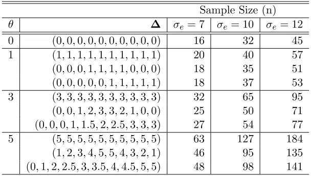
Table 2: Sample size calculations for the crossover design for 90% power with no random period effect (σp = 0)
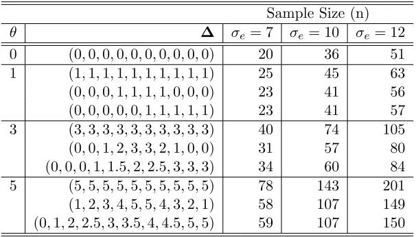
Table 3: Sample size calculations for the crossover design for 90% power with random period effect (σp = 4)
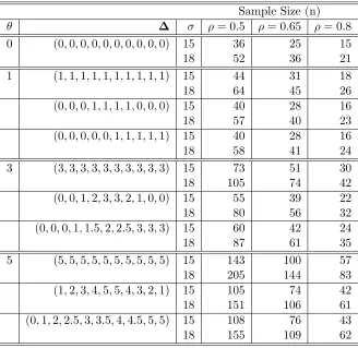
Table 4: Sample size calculations for the crossover design for 90% power given overall σ with ρ1 =ρ2
Sample Size (n) θ ∆ σ ρ= 0.5 ρ= 0.65 ρ= 0.8 0 (0,0,0,0,0,0,0,0,0,0) 15 36 25 15
18 52 36 21
1 (1,1,1,1,1,1,1,1,1,1) 15 44 31 18
18 64 45 26
(0,0,0,1,1,1,1,0,0,0) 15 40 28 16
18 57 40 23
(0,0,0,0,0,1,1,1,1,1) 15 40 28 16
18 58 41 24
3 (3,3,3,3,3,3,3,3,3,3) 15 73 51 30
18 105 74 42
(0,0,1,2,3,3,2,1,0,0) 15 55 39 22
18 80 56 32
(0,0,0,1,1.5,2,2.5,3,3,3) 15 60 42 24
18 87 61 35