Copyright2000 by the Genetics Society of America
Genetic Basis of Climatic Adaptation in Scots Pine by Bayesian
Quantitative Trait Locus Analysis
Pa¨ivi Hurme,* Mikko J. Sillanpa¨a¨,
†Elja Arjas,
†Tapani Repo
‡and Outi Savolainen*
*Department of Biology, FIN-90014 University of Oulu, Finland,†Rolf Nevanlinna Institute, FIN-00014 University of Helsinki, Finland and‡Faculty of Forestry, University of Joensuu, FIN-80101 Joensuu, Finland
Manuscript received January 3, 2000 Accepted for publication June 27, 2000
ABSTRACT
We examined the genetic basis of large adaptive differences in timing of bud set and frost hardiness between natural populations of Scots pine. As a mapping population, we considered an “open-pollinated backcross” progeny by collecting seeds of a single F1tree (cross between trees from southern and northern
Finland) growing in southern Finland. Due to the special features of the design (no marker information available on grandparents or the father), we applied a Bayesian quantitative trait locus (QTL) mapping method developed previously for outcrossed offspring. We found four potential QTL for timing of bud set and seven for frost hardiness. Bayesian analyses detected more QTL than ANOVA for frost hardiness, but the opposite was true for bud set. These QTL included alleles with rather large effects, and additionally smaller QTL were supported. The largest QTL for bud set date accounted for about a fourth of the mean difference between populations. Thus, natural selection during adaptation has resulted in selection of at least some alleles of rather large effect.
T
HE genetic basis of adaptive variation in natural mainly on domesticated species (see references in Tanksley 1993), but these studies do not relate the populations is still largely unknown.Fisher(1930)QTL effects to those segregating in natural populations. suggested that natural selection would fix alleles
confer-Moderately large QTL effects in natural populations ring small effects at a large number of loci. Later work
have been found for frost tolerance inEucalyptus nitens byKimura(1983) and Orr(1998) has shown that in
(Byrneet al.1997), and large effects have been found fact the mutations fixed during an adaptive process due
for flowering time inArabidopsis thaliana(Clarkeet al. to directional selection are not expected to be uniformly
1995;Mitchell-Olds1996;Kuittinenet al.1997) and small, but larger effects are fixed first. Fisher ignored
for bud flush in a cross between Populus species ( Brad-the fact that advantageous mutations of small effect are
shawandStettler1995). These and other studies in more susceptible to the effects of drift while they are
trees have been recently reviewed bySewellandNeale still rare. Later work byOrr(2000) has completed the
(1999). picture and further emphasized that the effects of
muta-We have attempted to examine the genetic basis of tions that are fixed are not likely to be very small.
adaptation to climate in Scots pine (Pinus sylvestris), Counter to the prevailing understanding, existing
em-which ranges from Spain (38⬚N) in the south to north-pirical studies provide evidence that many adaptations
ern Finland (68⬚N), and from western Scotland (6⬚W) could be based on even single loci, as reviewed byOrr
to eastern Siberia (135⬚E; Mirov1967). Scots pine is andCoyne(1992). Early studies relied on quantitative
wind pollinated with very efficient pollen flow (Koski analysis of line crosses using variants of the
Castle-1970). The whole range of Scots pine seems to be part Wright estimator of the number of segregating loci
of a panmictic population. Allelic frequencies are homo-(LynchandWalsh1998). With the advent of
molecu-geneous at marker loci, withFSTof 0.03 at isozyme loci lar markers and dense maps (e.g., Tanksley 1993),
between Sweden and eastern Siberia (Wanget al.1991). more powerful tools have become available. For
infer-Between northern and southern Finland,FST⫽0.02 for ring the genetic architecture underlying adaptation,
allozymes and restriction fragment length polymor-variation within or between populations needs to be
phisms (Karhu et al. 1996). Scots pine thus has an studied.
effectively infinite population size, and the population Few such data are available, as quantitative trait locus
structure corresponds to the model assumed byFisher (QTL) mapping studies on adaptive traits have been
(1930).
However, the environmental variation within this large range is enormous. Even within Finland, there is
Corresponding author:Pa¨ivi Hurme, Department of Biology, P.O. Box
a steep climatic gradient. In southern Finland the length
3000, FIN-90014 University of Oulu, Finland.
E-mail: [email protected] of the growing season (days with average temperature
MATERIALS AND METHODS ⬎5⬚) is ⵑ170 days at latitude 60⬚N and in northern
Finland⬍120 days at latitude 69⬚N. Scots pine colonized Pine material:The mapping population was derived as fol-these areas⬍10,000 years ago, after glaciation (Hyva¨ri- lows. The Finnish Forest Research Institute has its clonal archives (vegetatively reproduced trees) in Punkaharju nen1987). The colonization has required a major
adap-[61⬚48⬘N, 29⬚19⬘E; 90 m above sea level (a.s.l.)]. A tree of
tive shift in relation to the length of the growing season.
northern origin (P315, Kemija¨rvi, 66⬚35⬘N) had been crossed
This has led to population differentiation in many
with a southern tree (E1101, Punkaharju, 61⬚48⬘N), and the F1 growth-related traits, such as timing of vegetative growth trees had been planted in Loppi (southern Finland, 60⬚37⬘N, and frost tolerance (see references inSavolainenand 24⬚26⬘E; 100 m a.s.l.). We collected open-pollinated seeds Hurme1997). Reciprocal transfer experiments indicate from one of the F1 progenies in the spring of 1994. Thus,
QTL detection is based on observing marker genes in the
that such differences have a genetical basis (Eiche1966;
maternal component only. Erikssonet al.1980;Beuker1994). In common garden
The experiment was conducted twice, first in 1994 and the
experiments, growth cessation, terminal bud set, and
second time in 1996. In both years, the backcross progeny
frost hardening of young seedlings (and of adults) take and four population samples (Salla, Sotkamo, Kerima¨ki, and place earlier in northern than in southern populations Bromarv) ranging in latitude from 60⬚ to 67⬚N in Finland were included. By using population samples as controls, we
(Mikola1982;Toivonenet al.1991;Aho1994;Hurme
were able to observe the phenotypic variation of the backcross et al.1997). The genetic differentiation between
popula-progeny in relation to geographical variation in the same
tions is very high, as⬎80% of total genetic variation in
growing season. Seeds from the populations were bulk samples
bud set date is found between northern and southern from the forests of the Finnish Forest Research Institute. populations (Hurme1999). Differences in quantitative In both years, in the beginning of June, 450 seeds from the
backcross and 450 seeds from each control population were
traits are likely due to natural selection. The
homogene-sown in the greenhouse in Punkaharju Forest Research
Sta-ity of neutral markers shows that population
substructur-tion. The plants were arranged in 10 blocks, with each tray
ing or drift cannot have a major role.
consisting of 45 seedlings from a backcross or one of the
The outcrossing mating system of forest trees gives populations. Seedlings were grown under natural daylength rise to problems in QTL mapping. Populations may not and ambient temperature, except that the temperature was be fixed for different alleles, and many different alleles not allowed to decline below⫹5⬚.
Scoring bud set and frost damage:Timing of growth in
first-may segregate within and between populations. F2
prog-year pine seedlings is a reflection of general climatic
adapta-eny would be the best mapping population for
outcross-tion. The differences between the populations may be
ex-ing species. In forest trees, however, the types of map- pected to be found also in older populations of Scots pine. ping populations used are largely determined by the At least inPicea abies, the bud set dates of populations of 1- to pedigrees available, as obtaining multiple-generation 6-year-old seedlings were correlated over years (Ununger et al.1988;Ekberget al.1994), and inPinus contortaandPicea pedigrees takes decades in many species. Methods for
sitchensis, evidence of similar correlations of growth cessation
F2require either genotypic information from
grandpar-with latitude has been obtained in adult trees as well (Cannell ents or known haplotypes from parents. If these are not
andWillet1975).
available, it is possible to apply the methods developed First-year pine seedlings, grown in the greenhouse in south-byJansenet al.(1998) andSillanpa¨a¨andArjas(1999). ern Finland, will set an easily visible terminal bud toward the end of the summer. Bud set was scored twice per week from Sillanpa¨a¨andArjas(1999) devised a Bayesian method
the beginning of August to the end of October in 1994, and
that combines parameter estimation and model
selec-until October 10 in 1996. The date of bud set was scored as
tion (corresponding to different numbers of QTL) in
the number of days from sowing to the date when an
unambig-an efficient way. uous bud could be seen from above the seedling. Germination
We examine here the genetic basis of variation in occurred within a week in all seed lots. There was no latitudinal timing of bud set and development of frost hardiness variation, and variation in germination date did not contribute
to variation in bud set date.
in Scots pine. The very high differentiation between
Frost hardiness was studied in 1996 by exposing all seedlings
northern and southern Finnish natural populations
pro-of the backcross progeny to a predetermined freezing
temper-vides the starting point for QTL dissection. F2or back- ature during the frost hardening period. The frost treatment cross progenies are not available for Scots pine, but took place on October 8–9 when most of the buds had been we were able to obtain an “open pollinated backcross” formed. Frost damage of seedlings was based on visual scoring
of needles.
progeny (two-generation half-sib progeny) by collecting
For the frost treatments, a treatment temperature causing
seeds from a single F1tree (a cross between trees from
intermediate frost damage (LT50⫽50% needle damage) for southern and northern Finland) growing in southern
the backcross progeny was determined in advance. Eight
back-Finland. We have modified slightly the method ofSil- cross seedlings were tested at each of six temperatures (⫹5, lanpa¨a¨andArjas(1999) to fit this design. We compare ⫺4,⫺12,⫺22,⫺34, and⫺46⬚), and level of frost damage for needles was determined with the electrolyte leakage method
the size of the QTL effects we detected in this one
(Repo et al.1994; Hurmeet al.1997). The inflection point
pedigree to the variation found between and within
of the temperature response curve was recorded as the LT50 natural populations. Studying only one cross of course
temperature. LT50in the backcross was⫺24⬚, but since freezing limits the conclusions. Our other goal was to compare testing of all seedlings was done 1 wk after preassessments, Bayesian methods of mapping and effect estimation to additional hardening was assumed to have taken place. The
freezing temperature was chosen to be⫺28⬚.
The preassessments and the frost treatment to all seedlings in the regression model. Four block levels (combination of 10 blocks into 4) were used to indicate the locations of the were carried out in air-cooled chambers (ARC 300/⫺55⫹20,
Arctest, Finland). The freezing programs started at 10⬚and the seedling trays in the greenhouse. One marker was considered at a time and individuals with missing genotypes or phenotypes temperature was gradually cooled to the target temperature at
a rate of 5⬚/hr. The minimum temperature lasted 4 hr, after were omitted. For bud set, the single-marker analysis was done separately for 1994 and 1996.
which the temperature was raised back to 10⬚at 5⬚/hr. After
the frost treatments were applied to all plants, they were trans- The results were also used for choosing marker covariates to control background variation in the Bayesian QTL analysis. ferred to a greenhouse and kept at 22⬚/15⬚(day/night), with
a long photoperiod of 18 hr/6 hr (day/night). Needle damage A similar principle is also used in composite interval mapping
(Jansen1993;Zeng1993, 1994;JansenandStam1994). In
to the seedlings was scored 10 days after freezing, on a visual
scale from 0 to 10, where 0 is no injury and 10 is complete each data set, one significant marker from each linkage group showing potential effects (Pⵑ0.05) was selected as a back-injury (all needles brown).
Randomly amplified polymorphic DNA amplifications and ground control. For bud set, seven and eight background controls were used in years 1994 and 1996, respectively. For map construction:A randomly amplified polymorphic DNA
(RAPD) map was constructed as a basis for single-marker map- frost hardiness data, four markers were used (see Figure 2).
Bayesian analysis:Sillanpa¨a¨andArjas(1999) presented a ping and for choosing marker cofactors for Bayesian QTL
analysis (see below). Conifer seeds have haploid megagameto- hierarchical Bayes model for the QTL mapping of outcrossing species, where the number of QTL in the analyzed linkage phyte storage tissue surrounding the developing embryo. The
megagametophyte has the same genotype as the egg cell. As group as well as the unobserved (parental) linkage phases and missing incomplete marker genotypes were all treated as the seed germinates, the megagametophyte can be collected
off the developing seedling, and it yields sufficient DNA for random variables with unknown values. In this model, some QTL effects from other linkage groups are controlled for by a large number of PCR reactions. In this way, we could assess
the genotypes of the female gametes produced by the heterozy- using marker covariates representing potential QTL. During the estimation procedure, the model parameters (such as the gous F1maternal tree. A RAPD map (Williamset al. 1990)
was constructed from a sample of 84 megagametophytes inde- number of QTL, their locations, genotypes, and the corre-sponding phenotypic effects) are all updated according to a pendent of the phenotype collected off the seedlings of the
backcross progeny. Methods for RAPD reactions are described Markov chain Monte Carlo (MCMC) sampling scheme, even-tually resulting in dependent samples from the posterior
distri-inHurmeandSavolainen(1999).
Those loci where the megagametophyte genotypes segre- butions of these parameters. The Bayesian inference is then based on conclusions drawn from these samples.
gated 1:1 (2test) in the 84 backcross progeny were chosen for
mapping. The RAPD map was constructed with MAPMAKER/ Bayesian QTL analyses were executed with a modified (see
appendix) C program (Multimapper/OUTBRED;Sillanpa¨a¨
Exp 3.0 (Lander et al. 1987) using the Haldane mapping
function. Grouping was done with LOD 4.0 and maximum and Arjas1999), assuming a known marker map (see map construction above) but unknown maternal linkage phases. interval 50 cM ( ⫽0.31) as thresholds, after which multipoint
analysis was performed with log-likelihood differenceⱖ3 for The linkage phases estimated for the marker map were not utilized here, because a smaller offspring data set was used in framework markers. Other markers were located in relation
to the framework. All potential scoring errors given by MAP- estimating the marker map. For each linkage group of each data set, the method was run 2 ⫻ 106 cycles in the DEC
MAKER were verified, scoring uncertain double recombinants
as missing data. ALPHA 21164/437MHz processor at the Center for Scientific
Computing of Finland. No initial sample value was rejected Mapping the QTL: The QTL analyses for bud set were
made separately for years 1994 and 1996. For improved QTL because of starting-value dependency (burn-in), but the chain was thinned because of limited storage capacity so that only detection efficiency, selective genotyping was used (Lander
and Botstein 1989; Darvasi and Soller 1992; Tanksley every 10th iteration was saved.
In the preprocessing, all haplotypes of the offspring and 1993). On the basis of phenotypic information from the
seed-lings in the backcross progeny, seedseed-lings from the tails of the genotypes of the mother tree were already known based on the experimental design, but the possible alleles of the missing phenotypic distribution of bud set dates (years 1994 and 1996)
and frost damage scores (year 1996) were used, while seedlings diploid offspring genotypes and their origins were completed by using genotyping rules of Wijsman (1987). Technically in the middle of the distribution were not genotyped. All
markers with minimum distance of 1 cM in the RAPD map (see Appendix A inSillanpa¨a¨andArjas1999), the known homozygote genotype was artificially given to all marker loci in were amplified for the extremes as well.
In 1994, we had phenotypic data on 353 seedlings. RAPD the “synthetic father” to ensure that its assumed (background) contribution to the analysis was a constant. With this assump-markers were amplified from megagametophytes of 96
seed-lings from the extremes of bud set dates (48 early and 48 tion, the environmental contribution of the variance was in-flated by the paternal additive genetic contribution, with a late). Altogether, the 1994 data contained genotypes on 171
seedlings (of which 16 had missing phenotypes), including corresponding decrease in the additive genetic variance. This is a simplifying assumption, which does not quite hold (but the random individuals used for RAPD map construction in
addition to the extremes of selective genotyping. The 1996 note that 85% of the total variation was between the northern and southern grandparental populations, Salla and Kerima¨ki; data consisted of 405 phenotyped individuals, of which 96
extreme individuals were genotyped. The data sets 1994 and see below). For the mother tree, a known heterozygote geno-type was given to all loci with unknown linkage phases. 1996 were also analyzed together. The results on the combined
analysis are reported later only in part. For frost hardiness in The same environmental covariate (block) as in the single-marker analysis was also used here. The initial value of the 1996, we had phenotypic data for 379 individuals, of which
92 (46 low and 46 high) from both tails of the distribution number of QTL was three, with the corresponding loci evenly placed along the linkage group to be mapped. Following Sil-were genotyped.
Single-marker analysis:Single-marker analysis (ANOVA) was lanpa¨a¨andArjas(1998, 1999), the Poisson mean was set to two and the maximum number of QTL in one linkage group used for preliminary mapping. This analysis was done as a
able on these. The residual standard deviation was chosen to assumed known (same as those used in the ANOVA estima-tions). We applied either the single-QTL model or the two-be uniform over ranges [0, 13.37], [0, 15.91], and [0, 3.27]
for bud set data from 1994 and 1996, and frost hardiness, QTL model enlarged with the background controls and an environmental block effect. Additive effect estimates (median respectively. The right endpoint of the interval was the
pheno-typic standard deviation of the particular data set. The prior and 2.5 and 97.5% quantiles) were determined from the poste-rior cumulative distribution function of the phenotypic effects. of the intercept for bud set (frost hardiness) was chosen to
be uniform on [⫺200.0, 200.0] ([⫺40.0, 40.0]) and those of This was constructed as the expectation over the range of phenotypic effects associated with the different locations in the the QTL genotypic effects were independent normal
distribu-tions with mean zero and variance 2000 (400). The priors of marker interval flanking the particular QTL. Genetic variance estimates (median and quantiles) were likewise determined the background control effects were uniform on [⫺200.0,
200.0] ([⫺40.0, 40.0]). The prior of the QTL location was as the expectations over the range of genetic variance associ-ated with the different locations in the interval. QTL effect uniform between zero and the length of the analyzed linkage
group. The following proposal distributions were chosen on sizes were calculated from Bayesian estimation in two ways: directly from the genetic variances and indirectly from the the basis of several test runs. The random walk proposal ranges
(symmetric uniform density around previous value;Chiband additive effects. In the indirect estimation, the additive effects were used to estimate genetic variances and QTL effect sizes.
Greenberg1995) in the MCMC analyses were chosen to be
2.0 (location), 5.0 (intercept), 1.0 (residual SD), 7.5 (QTL Epistasis and genotype⫻environment interactions: Interac-tions between marker loci closest to putative QTL were tested coefficients), and 10.0 (cofactor coefficients) for bud set. The
corresponding values applied to the frost hardiness data were with ANOVA for epistasis. Markers and a block were the main effects, and an interaction term between one marker pair at one-tenth of those for bud set, except for location, which was
2.0. The proposal distributions for the genotypic effects of a time was included.
Genotype⫻environment interactions were studied for bud bud set and frost hardiness were chosen to beN(0, 10.0) and
N(0, 2.5) in cases where the addition of a new QTL to the set between years 1994 and 1996. All the markers closest to the putative QTL (one per QTL) were studied. The analysis model was proposed.
Estimating QTL effects:We estimated QTL effects using was done with nested ANOVA with an interaction term be-tween marker and year included. One QTL was tested at each haplotype information (megagametophytes) from random
sets of seedlings in each year to avoid overestimation of QTL time, and the whole model consisted of a marker, year, block (year), and the interaction term marker⫻year.
effects due to selective genotyping and genotype⫻ environ-ment interactions (LandeandThompson1990;Melchinger et al.1998).
In 1994, these seedlings included the random sample with RESULTS
respect to the quantitative traits used for RAPD map
construc-tion (84 seedlings) and an addiconstruc-tional random set, giving a Bud set dates and frost damage scores: The control total of 113 seedlings. In 1996, a random set of 115 megagamet- population samples (Salla, Sotkamo, Kerima¨ki, and Bro-ophytes was genotyped. For frost hardiness, 113 random
seed-marv) showed regular clinal latitudinal variation in bud
lings were included.
set in both years, and population differences were
sig-The additive effects of the putative QTL were first estimated
from regression coefficients from ANOVA. The model in each nificant (F⫽84.4d.f.⫽3,P⬍0.001 andF⫽629d.f.⫽3,P⬍
data set included markers closest to the QTL (one marker 0.001, in 1994 and 1996, respectively; see Figure 1). The per QTL) and a block effect. The regression coefficient of difference in the median date of bud set between the the marker genotype gives the difference between the two
northernmost and the southernmost populations (Salla
QTL genotype effectsAa-aa.The signs of the estimates were
and Bromarv) was ⵑ22 days in 1994 and 38 days in
determined by their estimated marker phases in the mother
tree, which had to correspond to the ones in the RAPD map. 1996. The difference between the two grandparental
This is because the origins (northern or southern grandpar- populations of the backcross (Salla and Kerima¨ki) was ent) of the RAPD alleles in the backcross progeny determine 15 days in 1994 and 28 days in 1996. The proportion whether genotype class 0 (or 1) is homozygote (aa) or
hetero-of the total variance between the two grandparental
zygote (Aa) at the respective QTL locus. The genetic variance
populations was 48% in 1994 and 85% in 1996. In 1994,
associated with each QTL was calculated as [(Aa-aa)/2]2, and
the relative QTL effect size was estimated by dividing the the bud set period was shorter, and the populations
genetic variance estimate by the phenotypic variance estimate overlapped in bud set. In 1996, the bud set periods of
of the random sample. the populations were not longer than in 1994 (similar
A second way to estimate the QTL effects was to estimate
variances), but the populations overlapped less in 1996
a coefficient of determination (R2) with ANOVA. The full
than in 1994.
model in each data set included markers closest to the QTL
(one marker per QTL) and the block effect. The effect of In the backcross progeny, the median date of bud set
one QTL at a time was studied by excluding the respective was 103 (September 12) in 1994 with SD 10.3. In 1996, marker from the model. The R2of this reduced model was
the median date of bud set was 94 (September 6) with
subtracted from theR2of the full model, giving an estimate
SD 10.1. The bud set of the backcross was intermediate
of the effect of the respective marker. The effect of all markers
between the grandparental populations (Figure 1). The
was obtained by subtracting theR2of the model where only
the block effect was included from theR2of the full model. backcross progenies and the grandparental populations
A third approach for estimating phenotypic effects was by overlapped more in 1994 than in 1996, consistent with restricting the Bayesian model to only those chromosomal comparison of the population samples.
regions that showed elevated posterior QTL intensity in the
The frost damage scores of the backcross progeny
Bayesian analyses. Two flanking markers around each putative
after frost treatment in⫺28⬚in October 1996 were
dis-QTL were genotyped in each random sample and the linkage
to the left (Figure 1). The average frost damage score found with 74 RAPD primers (2.4 polymorphic loci/ primer), but 12 (6.7%) of them showed segregation was 6.9 with SD⫽2.1.
Log-transformation did not make any of the distribu- distortion and were excluded. Finally, the RAPD map contained 164 RAPD markers, distributed in 16 linkage tions of bud set or frost damage more normal, so
un-transformed data were used in the QTL analysis. groups (Figure 2), and 3 markers remained unlinked. There were 12 large groups (from 35 to 136 cM),
corre-RAPD map: Altogether 179 polymorphic loci were
sponding to the haploid chromosome number of pines (n ⫽12), and 4 smaller ones (from 2 to 11 cM). The map spans 1000 cM, covering about half of the genome, estimated with the method of Chakravarti et al. (1991). Spacing between markers varied from 1 to 31 cM, with an average of 9.5 cM.
QTL mapping with Bayesian analysis: The posterior
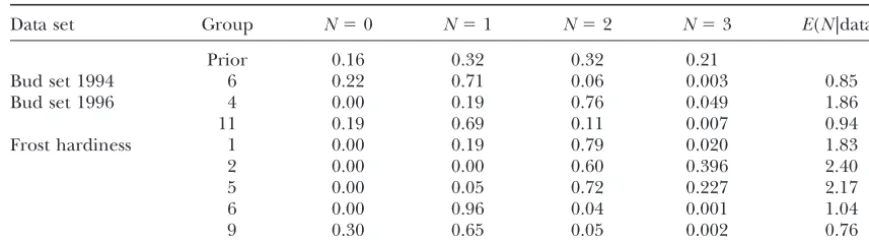
probability distributions for the number of QTL summa-rized potential QTL activity in each linkage group (Ta-ble 1). Here, the presence of one or more putative QTL in a linkage group was inferred, when the posterior probability for one or more QTL (Nⱖ 1) was at least two times the probability for the absence of a QTL (N⫽ 0). In this way, the estimated number of QTL per linkage group [E(N|data)] ranged between 0.76 and 2.40. The localization of the QTL was shown by the QTL intensity curves, where the relative frequency of QTL indications is visualized along each linkage group (Figure 3).
QTL activity for bud set in 1994 was found in linkage group (LG) 6 in the 1994 data, and in LGs 4 and 11 in 1996 (Table 1, Figure 3). In the combined data, QTL found in the separate data sets were also found, and additionally 1 putative QTL in LG 5 (Figure 3). The 1996 data indicated even the possibility of 2 QTL (poste-rior expectation 1.86 QTL) inside an area of 1.5 cM in LG 4, which may as well indicate 1 larger QTL.
QTL activity for frost hardiness was detected in link-age groups 1, 2, 5, 6, and 9, with two QTL in LGs 1, 2, and 5 (Table 1, Figure 3). The QTL in linkage groups 1 and 2 were clearly separated from each other, but close to each other in LG 5, possibly indicating a single QTL. Linkage groups 5 and 6 showed QTL activity for both bud set and frost hardiness. In LG 5 the QTL were clearly separated, but were close to each other in LG 6. No other genetic association between the traits was found, corresponding to the low phenotypic correlation (0.24).
Figure1.—(A) Frequency distributions of date of terminal
TABLE 1
Bayesian posterior probability distributions for the numbers of QTL
Data set Group N⫽0 N⫽1 N⫽2 N⫽3 E(N|data)
Prior 0.16 0.32 0.32 0.21
Bud set 1994 6 0.22 0.71 0.06 0.003 0.85
Bud set 1996 4 0.00 0.19 0.76 0.049 1.86
11 0.19 0.69 0.11 0.007 0.94
Frost hardiness 1 0.00 0.19 0.79 0.020 1.83
2 0.00 0.00 0.60 0.396 2.40
5 0.00 0.05 0.72 0.227 2.17
6 0.00 0.96 0.04 0.001 1.04
9 0.30 0.65 0.05 0.002 0.76
Groups with QTL activity are shown. Group refers to the linkage group,Nis the Bayesian posterior distribution of number of QTL, andE(N|data) the posterior expectation of number of QTL. Number of MCMC iterations was 2⫻106, and thinning of the chain was 10. The truncated Poisson prior distribution of number of QTL
is also shown.
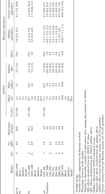
Single-marker analysis vs.Bayesian analysis:For bud With ANOVA the QTL effects calculated from R2
values ranged up to 12.7% for bud set and up to 11.1% set, all QTL supported by the Bayesian analysis were
also significant in the single-marker analysis. However, for frost hardiness, which were close to the estimates obtained from the ANOVA additive effects (Table 2). some additional marker areas were statistically
signifi-cant in the single-marker analysis. For instance, the QTL The estimates from the additive effects with the Bayesian method ranged up to 13.0% for bud set and up to 11.7% in LG 5 was found in single-locus analyses individually
in both the 1994 and 1996 data sets, but the Bayesian for frost hardiness. The largest QTL for bud set (effect 12.7% from ANOVA R2) was located in LG 4 in the analysis detected it only in the combined data set. Some
other cases of discrepancies are likely to have been false 1996 data. For frost hardiness, the largest QTL (11.1% from ANOVAR2) was located in LG 1 (Figure 3). The positives.
For frost hardiness, the methods performed differ- closely linked QTL for bud set and frost hardiness in LG 6 (distance of the peaksⵑ15 cM) had parallel effects ently. Single-locus analysis revealed only one significant
QTL in LG 1 (the one that proved to have the largest (positive signs; the later the bud set, the more frost damage). There may be two closely linked QTL or one effect on frost hardiness) and two marginally significant
QTL in LG 5 and LG 9. The Bayesian analyses found single pleiotropic QTL.
Altogether, based on the R2 values, the markers ex-two loci in LG 1 and several other QTL in other linkage
groups (see Table 1, Figure 3). In LG 1, the large plained 3.5 and 15.4% of the total phenotypic variation in the backcross bud set data from 1994 and 1996, re-amount of missing data in the flanking markers at the
other QTL may have led to low power and lack of sig- spectively. For frost hardiness, 24.9% of the variation was explained by the markers.
nificance in the single-marker analysis. The QTL in LGs
5 and 9 with the Bayesian analysis were at different Epistasis and genotype ⫻ environment interactions:
There was no evidence for epistasis. None of the interac-locations than indicated by the single-locus analysis.
QTL effects: The individual QTL effect estimates tions between marker pairs were significant in ANOVA
in any data set (data not shown). Nor did we find any were similar to the two methods based on ANOVA
(Ta-ble 2). The ANOVA estimates were also mostly similar genotype⫻ environment interactions at the QTL, but the tests had low power. However, the control popula-to the Bayesian estimates based on using additive effects.
A few larger differences occurred, however, in LG 6 in tions displayed significant population-by-year interac-tion (F⫽ 56.08d.f.⫽3,P⬍0.0001; see Figure 1). bud set data from 1994 and in frost hardiness.
Some individual QTL effects obtained from the ge-netic variances with the Bayesian method were very
dif-DISCUSSION
ferent from other estimates. The large credible regions
(quantiles) of the genetic variances resulted in inaccu- Size of factors underlying adaptive evolution in
natu-ral populations:As described in the Introduction, work
rate genetic variance estimates, and thus the QTL effect
sizes obtained from these estimates are not reported. byKimura(1983) andOrr(1998, 2000) has suggested
Figure2.—RAPD map of the F1tree (P315⫻E1101). Markers used as background control markers in the Bayesian analysis
that adaptation should be based on factors of larger size low proportion of the total phenotypic variation of the backcross in bud set date (15%) and frost hardiness than proposed byFisher(1930). Thus, during
adapta-tion, alleles with intermediate effects should be fixed (25%). However, our aim really was to compare the effects to genetic variation within and between popula-by natural selection. Fisher’s theory concerns especially
large continuous populations. On the basis of informa- tions, not to that of the backcross. The low proportion is accounted for by several reasons. First, there is much tion from neutral markers, Scots pine adaptation fits
this situation rather well. environmental variation in the backcross. Our earlier
quantitative genetics study gave within-population heri-We found two QTL in 1996 data, the effects of which
on bud set date were estimated as 4.5 and 3.1 days. tabilities of between 0.3 and 0.6 for southern and north-ern populations (Hurme1999). Further, we only knew These are the differences between the heterozygote and
the homozygote. As it is known from earlier studies that the marker results for the maternal parent and did not have any control over the paternal parent. Any variation there is little dominance (Mikola 1982; Hurmeet al.
1997 and references therein), the difference between contributed by the paternal parents will be included in the environmental variance. Last, the map did not have the two homozygotes at these loci would be 9 and 6
days, respectively. full genome coverage. Thus, some QTL likely have gone
undetected. These factors do not bias our estimates of We try to relate the size of these QTL to variation in
natural populations. Two of our four population sam- QTL effects. In fact, the single-locus estimates of QTL effects are more likely to be underestimates, because ples correspond to the populations of the grandparental
trees here, Salla and Kerima¨ki. The mean difference in recombination between the marker and the QTL will lower the effect estimates. Despite the limited power of bud set date between the two populations was 28 days.
Another quantitative genetics study, conducted with the experiment, the finding of relatively large effects compared to between-population differences or within-similar methods, in the same greenhouse, in the same
year, showed that the estimated additive genetic varia- population additive genetic variation will stand.
Comparison with QTL found in other organisms:In
tion in a southern population was 23.6 days2(based on
19 families with 40 progeny in each; Hurme 1999). comparison to most QTL mapping studies, there are three relevant aspects to this data set. First, we studied Thus, additive genetic standard deviation is 4.9. This is
the background against which we compare the sizes of natural populations, not influenced by human selec-tion. Second, we studied QTL responsible for within-the effects we found.
Fixation for alternative alleles in the north and south species differences. And most importantly, Scots pine is an outcrossing species. All of these factors could in-populations at these two loci alone (9 and 6 days) could
account for more than half the difference between the fluence our expectations of sizes of effects, but all of the factors could also influence the statistical power to grandparental populations. Note that the largest effect,
4.5 days, is close to the additive genetic standard devia- detect QTL. In outcrossers, background heterogeneity makes QTL detection more difficult, but if large differ-tion of the southern populadiffer-tion. Thus, effects at the
two individual loci could possibly account for a signifi- ences exist between parents, QTL can still be detected. There are only a few other studies on natural outcross-cant part of the between-population variation. Further,
the individual effects segregating between populations ing populations, where the differentiation was gener-ated by natural selection. In E. nitens, two QTL with (4.5 and 3.1 days) are rather large relative to the additive
genetic variance estimate within the southern popula- effects of 8 and 11% of the total phenotypic variation were found for frost tolerance (Byrne et al.1997). A tion. However, it is likely that we have not detected all
QTL even in this cross. In regions of the genome with direct comparison of the effects is not possible, as we do not know the heritabilities or differentiation between low coverage there may be loci with large effects, and
there will be smaller ones that we did not detect. Our parental populations. In Drosophila melanogaster, varia-tion in bristle number has been studied as a model trait conclusion is of course also limited because we only
analyzed one cross. However, in our view the important of quantitative variation, and alleles with large effects at a neurogenic locus,scabrous, govern variation within point is that we have demonstrated the existence of
alleles of relatively large effects at a few loci, even if we natural populations (Mackay and Langley 1990; Mackay1995). This locus explained 13 and 8% of the cannot estimate in what proportion of crosses such large
effects would be found. genetic variation in abdominal bristle number and
sternopleural bristle number, respectively,
demonstra-The proportion of variation in this backcross
ex-plained by the QTL:In all, the QTL accounted for a ting the segregation of alleles of large effect in natural
Figure3.—The approximate posterior QTL intensities represented as frequency polygons for bud set timing and for frost
populations (Lai et al. 1994; Long et al. 1995). Both 1998). In the greenhouse, this would mean different conditions between years due to ambient weather fluc-Drosophila and Scots pine are effectively outcrossing,
with very large effective population size, but compari- tuations or due to microenvironmental differences. The environmental variations clearly differed between years, sons are limited by different sampling (within vs.
be-tween population) and some differences in mating although there were no significant genotype⫻ environ-ment interactions. The control populations differed in system.
A priori, one could expect that breeders would have their reactions between years (P ⫽ 0.001), even if the ranking order of bud set was maintained. Other QTL efficiently selected for alleles with large effects and that
domesticated populations would differ by alleles with studies have provided evidence for G⫻ E interactions (e.g.,Jansenet al.1995).
larger effects than natural populations. Many QTL
stud-ies on crop plants do follow such a pattern (see refer- Evaluation of the Bayesian method: Sometimes in-bred line-cross (interval) methods are applied to out-ences inTanksley1993;LynchandWalsh1998). For
instance, in barley, frost tolerance loci accounted for bred data, even though many outbred methods (Haley et al.1994;MaliepaardandVan Ooijen1994;Jansen 31 or 79% of the variation in different years (Panet al.
1994). In the outcrossingBrassica rapa, smaller effects 1996;Knottet al.1997;Jansenet al.1998;Sillanpa¨a¨ andArjas1999) are available. This may lead to unrelia-have been found (Teutonico et al. 1995). Arora et
al.(1998) and Lim et al. (1998) suggested oligogenic ble results, since, in inbred methods, calculation of the QTL genotype probabilities is based on more restrictive inheritance for cold hardiness in cultivated blueberry
and Rhododendron. conditions for parental haplotypes. Interval methods
available for outbred half-sib designs (Georges et al. We could also expect to find larger effects in selfing
species rather than in outcrossers. In selfing populations 1995;Knottet al.1996) were not directly applicable to our design at the time we performed the analyses. Thus, with smaller effective population sizes, alleles with larger
effects (and more pleiotropic effects) could be fixed we analyzed the Scots pine data with the Bayesian out-bred method, which provided us a flexible multiple-due to drift. Indeed, in selfing A. thaliana, flowering
time differences between populations are largely due QTL model with background controls, where multiple testing problems could be avoided (Shoemaker et al. to one major gene and several minor ones (Clarkeet
al.1995;Mitchell-Olds1996;Kuittinenet al.1997). 1999). Therefore, the Bayesian method was considered to be most suitable for our data.
QTL fixed between species could be larger than
within species due to longer separation and possible The recently developed composite interval mapping method ofWu(1999) for megagametophytic informa-selection for reproductive isolation and QTL
differenti-ation. At the interspecific level, a cross between Populus tion could be applicable to our design. In Wu’s method the outcrossing rate and QTL genotype frequencies in species revealed five QTL influencing bud flush, which
explained 85% of the total variation (Bradshaw and the pollen pool are parameters to be estimated, whereas in our method these parameters were considered to be Stettler1995). For bud set,Frewenet al.(2000) found
four QTL with phenotypic effects between 6 and 12%, constants (homozygous pollen pool, outcrossing rate 100%). However, in Scots pine, empirical results in confirming these expectations.
Specific features of the study: The large size of the southern Finland suggest outcrossing rates ⵑ95–100%
(MuonaandHarju1989). backcross, ⵑ400 segregating progeny per year, was a
good starting point for an efficient study (see Mel- In our backcross, parental mating type (alwaysAa⫻ aa) and therefore marker informativeness are the same chingeret al. 1998). Considering the design, we had
two grandparents from different populations in the for all markers, which is similar to the inbred line cross case. Due to the same information content, different cross. Although the populations were differentiated,
they were each variable for bud set and frost hardiness chromosomal regions are treated equally in the analysis, and there is no tendency for QTL-intensity (or LOD-loci. Only part of this variation was introduced into the
cross, and only those loci heterozygous in the F1could score) graphs to be biased toward highly informative areas. For the same reason, the absolute values of a test be detected.
An important feature in the design was also the lack statistic from the single-marker analysis are also compa-rable between markers. However, incomplete marker of information on the paternal component. A constant
genetic effect from the father’s side was assumed in the coverage, unequal spacing, and missing genotypes may cause unbalance among chromosomal regions in the QTL analysis (fixed QTL in the pollen pool). We know,
however, that the pollen pool is variable, and this may analysis.
QTL effects with ANOVA and the Bayesian method:
decrease the power of the analysis.
The different bud set QTL found between years 1994 The estimates of largest QTL effects from ANOVA were congruent with the QTL effect size estimates from the and 1996 may have been due to environmental variance.
The interactions between QTL and the environment Bayesian method. In some other cases, the results ob-tained with the methods differed from each other (e.g., may influence the number and the size of QTL
Arora, R., L. J. Rowland, G. R. Panta, C.-C. Lim, J. S. Lehmanet
The two approaches, ANOVA and Bayesian
estima-al., 1998 Genetic control of cold hardiness in blueberry, pp.
tions, are not directly comparable. ANOVA estimations 99–106 inPlant Cold Hardiness:Molecular Biology, Biochemistry, and
Physiology, edited byP. H. LiandT. H. H. Chen.Plenum Press,
were performed by considering only the observed data
New York.
(omitting the missing data) and assuming that the QTL
Beuker, E.,1994 Long-term effects of temperature on the wood
resides at a marker locus. Due to these conditions, the production ofPinus sylvestrisL. andPicea abies(L.) Karst. in old
provenance experiments. Scand. J. For. Res.9:34–45.
standard errors were relatively small. Further, ANOVA
Bradshaw, H. D., Jr.,andR. F. Stettler,1995 Molecular genetics
estimates of QTL effects may be underestimates, since
of growth and development in Populus. IV. Mapping QTL with
the actual QTL location is usually at some distance from large effects on growth, form, and phenology traits in a forest
tree. Genetics139:963–973.
the marker. In the Bayesian estimation, on the other
Byrne, M., J. C. Murrel, J. V. Owen, E. R. Williams andG. F.
hand, uncertainty is incorporated by unknown positions
Moran,1997 Mapping of quantitative trait loci influencing frost
and unknown genotypes of QTL within the given tolerance inEucalyptus nitens.Theor. Appl. Genet.95:975–979.
Cannell, M. G. R.,andS. C. Willet,1975 Rates and times at which
marker regions, as well as by partly unknown maternal
needles are initiated in buds on differing provenances ofPinus
linkage phases. As a result, credible regions and
stan-contortaandPicea sitchensisin Scotland. Can. J. For. Res.5:367–
dard errors were different. In the Bayesian estimation, 380.
Chakravarti, A., L. K. LasherandJ. E. Reefer,1991 A maximum
it could also be seen that the second moments (such as
likelihood method for estimating genome length using genetic
variances) are not as well estimated as the first moments
linkage data. Genetics128:175–182.
(such as additive effects). The genetic variances from Chib, S.,andE. Greenberg,1995 Understanding the
Metropolis-Hastings algorithm. Am. Stat.49:327–335.
the Bayesian method did not fit well to the additive
Clarke, J. H., R. Mithen, J. K. M. BrownandC. Dean,1995 QTL
effects, but when these were estimated directly from
analysis of flowering time inArabidopsis thaliana.Mol. Gen. Genet.
the additive effect estimates, QTL-effect size estimates 248:278–286.
Darvasi, A.,andM. Soller,1992 Selective genotyping for
determi-similar to ANOVA effects were obtained.
nation of linkage between a marker locus and a quantitative trait
Some differences in the signs of the additive effects
locus. Theor. Appl. Genet.85:353–359.
obtained from ANOVA and Bayesian method were Eiche, V.,1966 Cold damage and plant mortality in experimental
provenance plantations with Scots pine in northern Sweden. Stud.
found. In most cases this can be explained by the small
For. Suec.36:1–218.
effects (additive effectsⵑ0). In bud set data from 1996,
Ekberg, I., G. Eriksson, G. Namkoong, C. NilssonandL. Norell,
the estimate of the sign of the additive effect (2.6) in 1994 Genetic correlations for growth rhythm and growth
capac-ity at ages 3–8 years in provenance hybrids ofPicea abies.Scand.
linkage group 11 with the Bayesian method depended
J. For. Res.9:25–33.
on which one of the flanking markers was assumed to
Eriksson, G., S. Andersson, V. Eiche, J. Ifver and A. Persson,
have a known linkage phase given by the RAPD marker 1980 Severity index and transfer effects on survival and volume
production of Pinus sylvestrisin Northern Sweden. Stud. For.
map. Comparison with the single-locus method
sup-Suec.156:1–31.
ported a positive effect.
Fisher, R. A.,1930 The Genetical Theory of Natural Selection.Oxford
The effects of some potential QTL found in the Bayes- University Press, Oxford.
Frewen, B. E., T. H. H. Chen, G. T. Howe, J. Davis,A. Rohdeet
ian mapping proved to be very small, ⬍1%. Yet these
al., 2000 Quantitative trait loci and candidate gene mapping
QTL were detected with Bayesian mapping. The main
of bud set and bud flush in Populus. Genetics154:837–845.
reason may be that different data sets (phenotypic ex- Georges, M., D. Nielsen, M. Mackinnon, A. Mishra, R. Okimoto
et al., 1995 Mapping quantitative trait loci controlling milk
pro-tremes in QTL mapping and random data sets in effect
duction in dairy cattle by exploiting progeny testing. Genetics
estimations) were used. These may have weighed the
139:907–920.
effects differently, possibly due to the pattern of distribu- Haley, C. S., S. A. KnottandJ.-M. Elsen,1994 Mapping
quantita-tive trait loci in crosses between outbred lines using least squares.
tion of missing data.
Genetics136:1195–1207.
We thank Teijo Nikkanen, Esko Oksa (The Finnish Forest Research Hurme, P.,1999 Genetic basis of adaptation: bud set date and frost Institute, Punkaharju Research Station), and Ville Pirttila¨ (Haapas- hardiness variation in Scots pine. Thesis, Acta Univ. Oul. A339. tensyrja¨ Tree Breeding Centre) for advice and help in obtaining the Oulu University Press, Oulu, Finland.
Hurme, P.,andO. Savolainen,1999 Comparison of homology and seed material and Jouko Lehto, Maija Rinkinen, and Sakari
Silven-linkage of random amplified polymorphic DNA (RAPD) markers noinen (The Finnish Forest Research Institute, Punkaharju Research
between individual trees of Scots pine (Pinus sylvestrisL.). Mol. Station) for their technical assistance. The Finnish Forest Research
Ecol.8:15–22. Institute, Punkaharju Research Station, and Haapastensyrja¨ Tree
Hurme, P., T. Repo, O. SavolainenandT. Pa¨a¨kko¨ nen,1997 Cli-Breeding Centre are acknowledged for supplying the seed material
matic adaptation of bud set and frost hardiness in Scots pine and the greenhouse facilities. We also thank Claus Vogl for theoretical (Pinus sylvestris). Can. J. For. Res.27:716–723.
discussions on relating QTL effects to variation between and within Hyva¨rinen, H.,1987 History of forests in northern Europe since natural populations. This study was financially supported by the Re- the last glaciation. Ann. Acad. Sci. Fenn. Ser. A III Geol.-Geogr. search Council for Agriculture and Forestry/Environment and Natu- 145:7–18.
Jansen, R. C.,1993 Interval mapping of multiple quantitative trait ral Resources, the Ministry of Education (Graduate School of
Evolu-loci. Genetics135:205–211. tionary Ecology), and the ComBi Graduate School.
Jansen, R. C.,1996 A General Monte Carlo method for mapping multiple quantitative trait loci. Genetics142:305–311.
Jansen, R. C.,andJ. Stam,1994 High resolution of quantitative traits into multiple loci via interval mapping. Genetics136:1447–1455. LITERATURE CITED
Jansen, R. C., J. W. Van Ooijen, P. Stam, C. ListerandC. Dean,
1995 Genotype-by-environment interaction in genetic mapping
Aho, M.-L., 1994 Autumn frost hardening of one-year-old Pinus
sylvestris(L.) seedlings: effect of origin and parent trees. Scand. of multiple quantitative trait loci. Theor. Appl. Genet.91:33–37.
mixture model approach to the mapping of quantitative trait loci tion of factors fixed during adaptive evolution. Evolution 52:
935–949. in complex populations with an application to multiple cattle
families. Genetics148:391–399. Orr, H. A.,2000 Adaptation and the cost of complexity. Evolution
54:13–20.
Janss, L. L., G. R. ThompsonandJ. A. M. Van Arendonk,1995
Ap-plication of Gibbs sampling for inference in a mixed major gene- Orr, H. A.,andJ. A. Coyne,1992 The genetics of adaptation: a reassessment. Am. Nat.140:725–742.
polygenic inheritance model in animal populations. Theor. Appl.
Genet.91:1137–1147. Pan, A., P. M. Hayes, F. Chen, T. H. H. Chen, T. Blakeet al., 1994
Genetic analysis of the components of winter hardiness in barley
Jensen, C. S.,andN. Sheehan,1998 Problems with determination
of noncommunicating classes for Monte Carlo Markov Chain (Hordeum vulgareL.). Theor. Appl. Genet.89:900–910.
Repo, T., M. I. N. Zhang, A. Ryyppo¨ , E. VapaavuoriandS. Sutinen,
applications in pedigree analysis. Biometrics54:416–425.
Karhu, A., P. Hurme, M. Karjalainen, P. Karvonen, K. Ka¨rkka¨inen 1994 Effects of freeze-thaw injury on parameters of distributed electrical circuits of stems and needles of Scots pine seedlings at
et al., 1996 Do molecular markers reflect patterns of
differentia-tion in adaptive traits of conifers? Theor. Appl. Genet.93:215– different stages of acclimation. J. Exp. Bot.45:823–833.
SAS,1987 SAS/STAT Guide for Personal Computers, Version 6.1 Edition.
221.
Kimura, M.,1983 The Neutral Theory of Molecular Evolution.Cam- SAS Institute, Cary, NC.
Savolainen, O.,andP. Hurme,1997 Conifers from the cold, pp. bridge University Press, Cambridge, UK.
Knott, S. A., J. M. ElsenandC. S. Haley,1996 Methods for multi- 43–62 in Stress, Adaptation and Evolution, edited byR. Bijlsma
andV. Loeschcke.Birkha¨user Verlag, Basel, Switzerland. ple-marker mapping of quantitative trait loci in half-sib
popula-tions. Theor. Appl. Genet.93:71–80. Sewell, M. M.,andD. B. Neale,1999 Mapping quantitative traits in forest trees, pp. 407–423 inMolecular Biology of Woody Plants,
Knott, S. A., D. B. Neale, M. M. SewellandC. S. Haley,1997
Multiple marker mapping of quantitative trait loci in an outbred edited byS. M. JainandS. C. Minocha.Kluwer Academic Publish-ers, The Netherlands.
pedigree of loblolly pine. Theor. Appl. Genet.94:810–820.
Koski, V.,1970 A study of pollen dispersal as a means of gene flow. Sheehan, N.,andA. Thomas,1993 On the irreducibility of a Markov chain defined on a space of genotype configurations by a sam-Commun. Inst. For. Fenn.70:1–78.
Kuittinen, H., M. J. Sillanpa¨a¨andO. Savolainen,1997 Genetic pling scheme. Biometrics49:163–175.
Shoemaker, J. S., I. PainterandB. S. Weir,1999 Bayesian statistics basis of adaptation: flowering time inArabidopsis thaliana.Theor.
Appl. Genet.95:573–583. in genetics: a guide for the uninitiated. Trends Genet.15:354–
358.
Lai, C., R. F. Lyman, A. D. Long, C. H. LangleyandT. F. C. Mackay,
1994 Naturally occurring variation in bristle number and DNA Sillanpa¨a¨, M. J.,andE. Arjas,1998 Bayesian mapping of multiple quantitative trait loci from incomplete inbred line cross data. polymorphisms at the scabrous locus ofDrosophila melanogaster.
Science266:1697–1702. Genetics148:1373–1388.
Sillanpa¨a¨, M. J.,andE. Arjas,1999 Bayesian mapping of multiple
Lande, R.,andR. Thompson,1990 Efficiency of marker assisted
selection in the improvement of quantitative traits. Genetics124: quantitative trait loci from incomplete outbred offspring data. Genetics151:1605–1619.
743–756.
Lander, E.,and D. Botstein, 1989 Mapping Mendelian factors Tanksley, S. D.,1993 Mapping polygenes. Annu. Rev. Genet.27:
205–233. underlying quantitative traits using RFLP linkage maps. Genetics
121:185–199. Teutonico, R. A., B. Yandell, J. M. Satagopan, M. E. Ferreira,
J. P. Paltaet al., 1995 Genetic analysis and mapping of genes
Lander, E., P. Green, J. Abrahamson, A. Barlow, M. Dalyet al.,
1987 MAPMAKER: An interactive computer package for con- controlling freezing tolerance in oilseedBrassica.Mol. Breed.1:
329–339. structing primary genetic linkage maps of experimental and
natu-ral populations. Genomics1:174–181. Toivonen, A., R. Rikala, T. RepoandH. Smolander,1991 Autumn coloration of first-yearPinus sylvestrisseedlings during frost
hard-Lim, C. C., R. AroraandS. L. Krebs,1998 Genetic study of freezing
tolerance in Rhododendron populations: implications for cold ening. Scand. J. For. Res.6:31–39.
Ununger, J., I. EkbergandH. Kang,1988 Genetic control and hardiness breeding. J. Am. Rhododendron Soc.52:143–148.
Long, A. D., S. L. Mullaney, L. A. Reid, J. D. Fry, C. H. Langley age-related changes of juvenile growth characters inPicea abies.
Scand. J. For. Res.3:55–66.
et al., 1995 High resolution mapping of genetic factors affecting
abdominal bristle number in Drosophila melanogaster. Genetics Wang, X.-R., A. E. SzmidtandD. Lindgren,1991 Allozyme differ-entiation among populations ofPinus sylvestris(L.) from Sweden
139:1273–1291.
Lynch, M. M.,andB. Walsh,1998 Genetics and Analysis of Quantita- and China. Hereditas114:219–226.
Wijsman, E. M.,1987 A deductive method of haplotype analysis in
tive Traits.Sinauer Associates, Sunderland, MA.
Mackay, T. F. C.,1995 The genetic basis of quantitative variation: pedigrees. Am. J. Hum. Genet.41:356–373.
Williams, J. G. K., A. R. Kubelik, K. J. Livak, J. A. Rafalskiand numbers of sensory bristles ofDrosophila melanogasteras a model
system. Trends Genet.11:464–470. S. V. Tingey,1990 DNA polymorphisms amplified by arbitrary
primers are useful as genetic markers. Nucleic Acids Res. 18:
Mackay, T. F. C.,andC. H. Langley,1990 Molecular and
pheno-typic variation in theachaete-scuteregion ofDrosophila melanogaster. 6531–6535.
Wu, R. L.,1999 Mapping quantitative trait loci by genotyping hap-Nature348:64–66.
Maliepaard, C.,andJ. W. Van Ooijen,1994 QTL mapping in a loid tissues. Genetics152:1741–1752.
Zeng, Z.-B.,1993 Theoretical basis of separation of multiple linked full-sib family of an outcrossing species, pp. 140–146 inBiometrics
in Plant Breeding: Applications of Molecular Markers, edited byJ. W. gene effects on mapping quantitative trait loci with the aid of genetic markers. Proc. Natl. Acad. Sci. USA90:10972–10976.
Van OoijenandJ. Jansen.CPRO-DLO, Wageningen, The
Neth-erlands. Zeng, Z.-B.,1994 Precision mapping of quantitative trait loci.
Genet-ics136:1457–1468.
Melchinger, A. E., H. F. UtzandC. C. Scho¨ n,1998 Quantitative trait locus (QTL) mapping using different testers and
indepen-Communicating editor:Z-B. Zeng
dent population samples in maize reveals low power of QTL detection and large bias in estimates of QTL effects. Genetics
149:383–403.
Mikola, J.,1982 Bud-set phenology as an indicator of climatic adap-tation of Scots pine in Finland. Silva Fenn.16:178–184.
APPENDIX
Mirov, N. T.,1967 The Genus Pinus.Ronald Press, New York.
Mitchell-Olds, T.,1996 Genetic constraints on life-history
evolu-Here we comment briefly on the order in which the
tion: quantitative-trait loci influencing growth and flowering in
Arabidopsis thaliana.Evolution50:140–145. updating of the MCMC algorithm takes place. There
Muona, O.,andA. Harju,1989 Effective population sizes, genetic are two strong dependency relations in the offspring variability and mating system in natural stands and seed orchards
data: the vertical dependency between parents and their
ofPinus sylvestris.Silvae Genet.38:221–228.
adja-cent loci in each individual. If single-site updating is way: With equal probabilities, the sampler does either a (1) family block update or an (2) individual update. applied, the sampler can easily get stuck in some part
of the sample space because of these dependencies
1. The family block update is similar as before, except (SheehanandThomas1993;Jansset al.1995;Jensen for step 2.5. In the new version, the grandparental andSheehan1998). To facilitate movement in the sam- origins are determined for offspring alleles having a ple space (mixing) of the MCMC sampler, especially in heterozygous parent, but are proposed directly from cases in which a large proportion of the data is missing the prior (Equation 4) for alleles inherited from and the markers are very close to each other, the follow- homozygotes. The acceptance ratio is then modified ing two-directional blocking scheme was implemented accordingly.
to the sampling algorithm of the Multimapper/OUT- 2. Individual update: Proposals covering the entire BRED program of Sillanpa¨a¨ andArjas (1999). This chromosome (all markers jointly) of each offspring modified program version is currently available on the are constructed (conditional on parents) similarly as web (http:/www.rni.helsinki.fi/ⵑmjs) and it was applied in step 2 ofSillanpa¨a¨andArjas(1999; Appendix
in all cases in this study. A), but their acceptance is tested separately for each
Step 2 in the sampling scheme ofSillanpa¨a¨andAr- haplotype proposal of each individual. The accep-tance ratio is again modified accordingly.