Statistical analysis of crossover interference using the chi-square model.

(1)

Copyright 0 1995 by the Genetics Society of America

Statistical

Analysis of

Crossover Interference

Using the Chi-square Model

Hongyu Zhao, Terence P. Speed and Mary

Sara

McPeek'

Department of Statistics, University of California, Berkeley, California 94720

Manuscript received December 17, 1993

Accepted for publication October 19, 1994

ABSTRACT

The chi-square model (also known as the gamma model with integer shape parameter) for the occurrence of crossovers along a chromosome was first proposed in the 1940's as a description of

interference that was mathematically tractable but without biological basis. Recently, the chi-square model has been reintroduced into the literature from a biological perspective. It arises as a result of certain hypothesized constraints on the resolution of randomly distributed crossover intermediates. In

this paper under the assumption of no chromatid interference, the probability for any single spore or tetrad joint recombination pattern is derived under the chi-square model. The method of maximum

likelihood is then used to estimate the chi-square parameter m and genetic distances among marker

loci. We discuss how to interpret the goodnessof-fit statistics appropriately when there are some recombination classes that have only a small number of observations. Finally, comparisons are made between the chi-square model and some other tractable models in the literature.

C

ROSSOVER interference has been observed in

almost all organisms studied, although there is little consistent evidence of chromatid interference even within the same organism (ZHAO et al. 1995)

.

In what follows we assume no chromatid interference (NCI)

.

Information on the distribution of crossovers along a chromosome generally comes from genetic experiments in which only recombinations, not crossovers, can actually be observed. In some organisms, such as Drosophila, the results of such experiments are in the form of single spore data, in which the products of a single meiosis are recovered separately. Other organisms, such as yeast, yield tetrad data, in which all four meiotic products are recovered together. It is easy to see that there are 2" distinct recombination patterns for single spore data involving n

+

1 markers. For tetrad data involving n

+

1 markers, n

>

1, there are more than 3" distinguishable tetrad patterns, but under the assumption of NCI, there are only 3 different probabilities among these patterns, i e . , some distinct tetrad patterns have the same probability of being observed. Each different probability corresponds to one of the types ( ilil * * i n ) , where ii = 0, 1, 2 corresponds to parental ditype, tetratype and nonparental ditype, respectively, between I] and li+l

.

Both single spore data and tetrad data record recombination events among a set of markers. As the underlying crossovers occurring during meiosis are not directly

Corresponding authm: Hongyu Zhao, Department of Statistics, Uni- versity of California, Berkeley, CA 94720.

E-mail: [email protected]

5734 University Ave., Chicago, IL 60637.

E-mail: [email protected]

'

Present address: Department of Statistics, University of Chicago,

Genetics 139 1045-10.56 (Febnrary, 1995)

observable from the data, any model about interference must relate the observable recombination or tetrad patterns to the underlying unobservable crossover events. Crossing over occurs among four strands after each homologous chromosome has duplicated. A model re- lating crossovers to recombination should specify the distribution of crossover points along the bundle of four chromatids and the choice of nonsister chromatids to be involved in each crossover.

The chi-square model for crossovers has a long history; see BAILEY (1961). MCPEEK and SPEED (1995) briefly review the history and fit a more general class of models, renewal processes with gamma interarrivals, which includes the class of chi-square models, to Dro- sophila data by maximum likelihood using a Monte Carlo method. Whereas it has generally been of interest due to its mathematical tractability, the chi-square model has also been suggested as a plausible biological model by Foss et al. (1993), motivated by observations from experiments on gene conversion. There the model is represented in the form

Cx(

Co) as follows: assume that crossover intermediates ( Cevents) are randomly distributed along the four-strand bundle, and every C event will either resolve in a crossover (

Cx)

or not ( Co)

.

When a C resolves as a Cx, the next m C's must resolve as Co events, and after rn Co's the next C must resolve as a

Cx,

i.e., the C's resolve in a sequence

-

* Cx( Co) Cx( Co) m -

-

. To make the process sta-

tionary given a set of C events, the leftmost C has an equal chance to be one of Cx( Co) m. In their paper Foss et al. estimate the parameter m in Cx( Co) from the observed ratio of Co to Cx. Here we perform a full maximum-likelihood estimation procedure to estimate

(2)

1046 H. Zhao, T. P. Speed and M. S. McPeek

ESTIMATION UNDER THE CHI-SQUARE MODEL

Given a set of markers l1,

. . .

,

I,,, along a chromosome, under the chi-square model Cx( Co) n

+

1 parameters need to be specified, namely, m and the genetic distances between each consecutive pair of markers, x l , x2,

. . .

, x,, so that the probability of each single spore or tetrad recombination pattern can be calculated. Suppose these parameters are given, let p = m

+

1, y, = 2pxj and let Dk ( y ) be the matrix whose i , jth entry is e-yypk+*-t/ ( p k

+

j

- i) !. Then the probability of

kj crossovers between . I, and . l i + l ,

j

= 1, * n , is (see APPENDIX, Lemma) :

1

- lDk, ( J I ) Dkp ( y 2

1

*

-

* Dk,,

( y n )

1 I , where

P

1 = ( 1 , 1 , .

. .

, l ) .

Note that when

P

= 1 , the above expression reduces to the Poisson case, i.e., the no-interference model of HALDANE (1919). Using the above formula, we can calculate the probability of any single spore or tetrad recombination pattern ( i l i p

-

* * in). We consider the two cases separately.

For single spore data, given two consecutive markers

l j and

1,+',

we can observe a recombination or nonre-

combination between them. If no crossovers occur between I, and

b+l,

no strand in the bundle will show any recombination between these markers. MATHER

(1935) proved that under the assumption of NCI, if there are k 2 1 crossovers between two markers, then the probability that these two markers recombine on any given single strand is Recall that for single spore data any recombination pattern can be represented as

( i l i 2 .

-

* i n ) , where i, = 0 or 1. Define

Nj = Do (yi)

+

' 1 2

C

Ds ( y j )

521

Rj

= ' / 2

C

Ds ( y j )

.

\> 1

Then the probability of recombination pattern ( ilie

-

- -

in) is (see APPENDIX, Theorem 1 )

1

P ( i l i 2 . * in) = - 1MIM2. ""1 I ,

P

where Mj = N j when

2;

= 0, and Mj = Rj when

2;

= 1. For tetrad data recall that there are three different possible tetrad patterns between two markers. We let

Po,

p ,

and

p,

denote the probabilities of parental ditype,

tetratype and nonparental ditype, respectively, between a fixed pair of markers. Given k 2 1 crossovers between two loci, under the assumption of NCI, the conditional probabilities

p g ) ,

p i k )

and

p i k )

of a tetrad being of parental ditype, tetratype and nonparental ditype, respectively, are given by MATHER (1935) :

pAk)

= l/3 ( l/2

+

( - l/2

1 p i k )

= z/:3(1 - ( - l / 2 ) k ,

p i k )

= l/3 ( l/2

+

( - ' / 2 )

.

We can calculate the probability of any tetrad pattern ( i l i 2 .

- -

i n ) , where il = 0, 1 or 2. Define

Pj = DO(y1)

+

C

' / 3 ( ' / 2

+

("/2)k)Ds(yl)

$ 2 2

Tj = Dl(rl)

+

'/:3(1 - ( - 1 / 2 ) k ) D s ( ~ l )

5 2 2

Nj ==

C

' / ' ~ ( ~ / ' z

+

( - ' / z ) k ) D s ( y j ) .

,=2

Then the probability of the tetrad pattern ( i l i 2 *

-

i,) can be written as (see APPENDIX, Theorem 2 )

1

P(iIi2. *

.

irL) = - 1M1M2. * * M n l ' ,

P

where Mj = P j if il = 0, Mj = Tj if il = 1, and Mj = Nj

if i, = 2.

Given a set of single spore or tetrad data and based upon the above formulae, the likelihood of the observations, up to a constant factor, can be calculated in terms of the parameters as

n

P ( i l i 2 . * * in)x'l'~i.".',,, where x i , z 2 . . is the observed frequency of single spores or tetrads with pattern ( i l i 2

- -

-

i,)

.

The maximum likelihood estimates of the parameters are those that max- imize the likelihood among all possible parameter values. The numerical method used to find the maximum likelihood estimates used in our analysis is the downhill simplex method, see PRESS et al. (1988). The standard error for each estimate is approximated using the fact that as n + m ,

&(eln

- 0,) + N ( O ,

[ m I ; ' L

where I ( 0 ) is the Fisher information matrix.

APPLICATIONS TO VARIOUS ORGANISMS

In this section the Cx( Co)" model is fitted to data from various organisms via the method of maximum likelihood. Data are of tetrad form except Drosophila melanogaster and human recombination data that are of single spore type.

Drosophila melanogaster: Many valuable recombina-

tion datasets for this organism have appeared in the literature since it was first studied by geneticists early in this century. Among these, two large, well-known datasets, namely WEINSTEIN (1936) and MORGAN et al.

(1935), have drawn much attention and have fre- quently been used as a basis upon which to compare different models.

Seven loci that cover most of the X-chromosome of

(3)

Chi-square Model

TABLE 1

Observed and expected counts under the cX( Co)" model

sc-e en,

0 0

1 0

0 1

0 0

1 1

1 0

0 1

0 0

1 1

1 0

0 1

0 0

1 1

cv-ct ct-u u-g gf

0 0 0 0

1 0 0 0

0 1 0 0

0 0 1 0

0 0 0 1

0 0 0 0

1 0 0 0

0 1 0 0

0 0 1 0

0 0 0 1

1 0 0 0

0 1 0 0

0 0 1 0

0 0 0 1

1 1 0 0

1 0 1 0

1 0 0 1

0 1 1 0

0 1 0 1

0 0 1 1

0 1 0 0

0 0 0 1

1 0 1 0

1 0 0 1

0 1 1 0

0 1 0 1

0 0 1 1

1 1 0 0

0 1 1 0

0 1 0 1

0 0 1 1

1 1 0 1

1 0 1 1

0 1 1 1

1 1 0 0

1 0 0 1

Expected Observed

12934 12776 1266 1407 1909 201 8

1831 1976 3420 3378 2454 2356 2119 2067

5 9

34 16

205 142

240 198

226 206

8 11

146 136

280 261 327 318

33 42

150 148

258 212

65 123

252 315

30 59

0 3

0 1

1 2

3 3

5 3

3 10

14 15

3 1

0 1

2 2

9 10

3 1

2 5

1 5

0 1

Cx( Co)' gives the best fit among Cz( Co) models. The estimated genetic distances and their standard errors between these markers are 7.13 2 0.14,9.55 -C 0.17,8.28 2 0.16, 14.75 ? 0.20, 11.45 2 0.18 and 11.47 2 0.19 cM. 0, no recombina-

tion; 1, recombination. The estimated P value is <0.001. Data

of WEINSTEIN (1936).

largest likelihood is achieved when the

Cx(

Co) model is used. The estimated genetic distances and their associated standard errors are given in Table 1. The optimal m = 4, estimated here by statistical analysis, is the same as that in F O ~ S et al. (1993), where they determine m from the observed proportion of gene conversions associated with crossovers.

MORGAN et uL's dataset also contains markers on the

X-chromosome of Drosophila. There are 16,136 observations on nine loci in this dataset, including six of the same loci as in WEINSTEIN ( 1936)

.

The Cx( C O ) ~ model

for Interference

TABLE 2

Estimated genetic distances with standard errors

under the cX( C O ) ~ model

1047

Distance

Interval ( C M ) SE

sc-e

en, cv-ct

ct-u

WS

S-f

f c a ca-b

5.13 9.83 7.49 13.29

8.42 15.55 7.47 4.42

0.17 0.23 0.20 0.26 0.21 0.28 0.20 0.16

Cx( C O ) ~ model gives the best f i t among Cx(Xo)= models. The estimated P value is <0.001. Data of MORGAN et al. (1935).

again gives the best fit to the data among the

Cx(

Co)" class. The results are given in Table 2. MCPEEK and SPEED (1995) fit a broader class of models, in which m is allowed to be noninteger, to the MORGAN et al. dataset and estimated m = 3.94, which agrees very well with the integer value m = 4.

Among the loci that appear in both datasets, the genetic distances estimated from the two different datasets appear rather similar, yet the differences are large com- pared to the standard errors. This difference probably reflects nonhomogeneity across Drosophila individuals. It is well known that recombination values are different for different individuals and can be affected by factors such as temperature ( PERKINS 1962)

.

However, in the

Cx(

Co) model we assume that the crossover process follows the same distribution across the whole popula- tion. Thus, it is not surprising that we underestimate the variation in genetic distances.

NeUrosjmra crmsa: PERKINS (1962) contains data in-

volving six markers on the right arm of linkage group I in N. uussu. PERKINS' data were gathered from six different experiments. This set of data was previously analyzed by COBBS ( 1978) and RISCH and LANCE (1983). In his paper PERKINS observes that there are significant differences between recombination values for offspring from different parents and from the same set of parents when the temperature is varied. We estimated the interference parameter m for each experiment separately and also for the data when all six experiments are combined. In all cases the best model is

Cx(

Co)" which has less crossover interference than

Cx ( Co) 4 . This suggests crossover interference is weaker

in Neurospora than in Drosophila. The results are given in Table 3.

There is another large multilocus Neurospora dataset

in STRICKLAND ( 1961 )

.

He accumulated data from four

(4)

1048 H. Zhao, T. P. Speed and M. S. McPeek

TABLE 3

Observed and expected counts under the Cx( Co)‘ model cr-th th-ni ni-uu au-ni ni-os Expected Observed

0 1 0 0 0 0 1 1 1 1 0 0 0 0 0 0 0 0 1 1 1 1 1 1 0 0 0 0 1 1 1 0 0 0 1 0 0 0 1 0 0 0 2 1 1 1 0 0 0 0 1 1 1 0 0 0 1 1 1 0 1 1 0 1 0 0 0 1 0 0 0 1 0 0 0 1 0 0 2 1 1 0 1 0 0 1 1 0 1 1 0 1 1 1 1 1 0 0 0 0 1 0 0 0 1 0 0 0 1 0 0 1 0 1 0 1 0 1 0 1 1 0 1 1 1 0 1 1 0 0 0 0 0 1 0 0 0 1 0 0 0 1 0 0 1 1 0 0 1 0 1 1 0 1 1 1 0 1 1 1

106 103

57 65

189 201

109 108

74 52

141 126

26 19

32 24

27 32

61 79

3 5

41 36

50 40

152 188

0 1

8 15

52 47

19 22

4 2

6 8

20 14

2 5

15 10

7 6

2 7

19 18

13 11

2 2

0 1

2 1

0 1

1 3

Cx( Co)’ gives the best fit among Cx( Co) models. The esti-

mated genetic distances with standard errors between these markers are 10.66 (0.59), 22.78 (0.82), 11.81 (0.60), 8.57 (0.55) and 21.69 (0.80) cM. 0, parental ditype; 1, tetratype; 2, nonparental ditype. The estimated P value is 0.69. Data of PERKINS (1962).

Cx ( Co) model to the data from each of the four experiments separately, and the Cx(

C O ) ~

model gives the highest likelihood in all cases. The results are summarized in Table

4.

As in the case of the Drosophila data, some of the estimated genetic distances are significantly different from one experiment to another.

BOLE-GOWDA et al. ( 1962) consider seven markers on linkage group I of Neurospora crassa, three on the left arm and four on the right arm. Altogether 2920 offspring were observed. When all markers are used in the analysis, the best model turns out to be

Cx,

i.e., m is estimated as zero. This estimate is inconsistent with the estimates from the data of PERKINS (1962) and STRICK- LAND (1961). This discrepancy might be due to the fact that no positive interference was observed across the centromere, and in that case the chi-square model may not be applicable to data which span the centromere.

The estimated m = 2 for Neurospora is consistent with the observation of the ratio of gene conversions to crossovers as described in Foss et al. ( 1993). Moreover, from the fact that

Cx(

C O ) ~

is the best

Cx(

Co) ” model for data from both linkage groups I and V, we might suspect that the degree of interference is similar within the entire Neurospora genome but with no interference across the centromere.

Saccharomyces cerevisiae: There are abundant two-

point cross data for S. cereuisiae, but, perhaps because of the high frequency of gene conversion, published multilocus tetrad data are rare. We analyze two-point cross data from a series of papers by MORTIMER and HAWTHORNE (1960, 1966,1968, 19’73). They were analyzed by SNOW (1979) using the model proposed by

BARRATT et al. ( 1954). In BARRATT’S model, there is

a parameter k that measures the degree of crossover interference, similar to the role m plays in the

Cx(

Co)

’’’

model. (For a full description, see BARRATT et al. 1954.)

k = 1 implies no interference, whereas k

>

1 and k

<

1 correspond to negative and positive interference, respectively. We say that there is positive (negative) interference if the probability of double recombinations in two intervals is less (bigger) than the product of the probabilities of recombination in each interval, ie., interference is defined through a quantity called S:3

by Foss et al. (1993)

.

SNOW fits BARRATT et al.’s model

to tetrad data involving 34 pairs of markers on 12 chromosomes in S. cueuisiae. SNOW’S results, along with our estimated optimal m , genetic distances and associated standard errors from the

Cx(

Co)” model, are given in Table 5.

Professor J. HABER kindly provided us with a multilo-

TABLE 4

Estimated genetic distances with standard errors and estimated P values

Experiment 1 Experiment 2 Experiment 3 Experiment 4

histl-inos 4.33 (0.33) 7.07 (0.40) 6.50 (0.35) 5.40 (0.29)

inos-bis 4.97 (0.36) 5.27 (0.35) 6.02 (0.36) 6.23 (0.32)

bis-pab2 10.1 (0.47) 9.18 (0.45) 10.7 (0.45) 10.6 (0.40)

P value 0.50 0.02 0.02 0.13

(5)

Chi-square Model for Interference

TABLE 5

Data of S. cereuiSiae analyzed in SNOW (1979)

Chromosome Gene pair m n x x 2 SE

P

X , k

1049 3 4 5 6 7

2 cyhl-gall

lys2-try1 SUP45-lyS2 gall-lys2 tryl-his7 SUP45-tyrl his4-mat1 h i s 4 - h 2 h 2 - m a t 1 matl-thr4 thr4-MAL2 SUP35-arol hid-trp2 ura3-hom3 SUP1 I-his2 trp5ade6 ade5-tyr3 try3-lys5 cyh2-trp5 h l - a d e 6 MAL 1 - d e 3

thrl-CUP1 CUPl-petl tql-cdc2

8 petl-CWl

9 his6lysl

10 SUP4-sw7

11 met1 4-met1

metl-MAL4 15 serl -ade2

ade2-qh4 pet1 7-ade2

17 met29ha2

pet2-pha2 1 2 3 5 2 0 2 1 1 1 2 5 1 2 5 1 0 1 0 3 2 1 3 3 3 1 2 1 1 4 1 2 2 1 146 383 335 127 104 105 278 521 48 1 434 286 101 205 215 206 105 106 166 162 160 507 138 232 486 240 41 1 179 109 133 210 236 232 146 151 19.9 52.7 34.8 42.2 25.7 17.4 39.8 17.4 35.8 21.3 29.2 46.1 18.2 24.5 34.7 22.0 82.1 73.3 8.0 44.8 34.3 52.0 46.7 24.4 36.0 47.1 53.1 46.2 28.0 27.4 33.9 48.8 36.8 50.7 2.6 3.5 1.9 3.5 3.1 3.4 2.8 1.2 2.2 1.6 2.2 7.5 2.1 2.2 2.3 3.2 4.9 1.7 3.9 1.8 6.4 3.4 1.3 2.6 3.3 5.4 6.1 3.4 2.0 3.0 3.9 3.5 5.9 10. 0.98 0.71 0.77 0.90 0.89 0.64 0.77 0.85 0.73 0.90 0.82 0.99 0.92 0.79 0.99 0.97 0.62 0.87 0.89 0.88 0.89 0.78 0.80 0.96 0.98 0.55 0.78 0.96 0.70 0.98 0.78 0.79 0.75 0.93 23.0 79.5 50.0 70.5 32.7 17.4 56.3 19.8 44.6 24.8 38.2 80.9 20.8 30.8 53.2 25.6 83.3 101. 0.80 70.5 46.7 68.5 74.7 31.8 52.4 61.1 80.1 59.7 33.5 37.5 41.9 72.8 50.6 66.4 0.337 0.488 0.245 0.194 0.258 1.817 0.294 0.370 0.429 0.404 0.294 0.204 0.284 0.277 0.115 0.386 1.333 0.764 2.355 0.265 0.271 0.495 0.271 0.112 0.210 0.461 0.498 0.545 0.633 0.098 0.397 0.367 0.386 0.551

m, estimated m in the Cx( C O ) ~ model; n, sample size; ~ 2 estimated genetic distance , from the Cx( Co)" model; SE, standard error for the estimated genetic distance;

p,

estimated Pvalue; x,, estimated genetic distance

in SNOW (1979); k, estimated k in BARRATT et aL's model in SNOW (1979).

cus S. cerevisiae dataset involving the five markers, metl3, qh2, t q 5 , q h 3 and leul on chromosome

VII.

The markers met13, qh2, t q 5 and leul were used in three of the 14 experiments, and metl3, t q 5 , q h 3 and leul were used in the other 11 experiments. We grouped the data across the experiments having the same set of markers and fitted chi-square models.

Cx( C O ) ~

gives the best fit

to the data from crosses involving metl3, qh2, t q 5 , q h 3

and leul; however, the best model for the other group is

CxCo.

The estimated Pvalues are 0.48 and 0.89, respectively.

Genetic experiments (Foss et al. 1993) have shown that in S. cerevisiae the ratio of gene conversions to crossovers is

-2,

so we might expect the model

Cx( Co)'

to fit best. From Table 5 and results for HABER'S data, we

can see that unlike Drosophila and Neurospora, where the optimal m does not change from one experiment to another, in Saccharomyces the optimal m varies for

different pairs of genes even within the same chromosome. With such a small sample size (usually -200), it may be that there is simply not sufficient information to clearly distinguish between different

Cx( Co)

models. In these Saccharomyces crosses the differences between the likelihoods under different

Cx

(

Co)

models are usually small. For example, for the second group

in IIABER's data, the -log( 1ikelihood)'s are rather

close for different m's: they are 125.6, 125.3, 125.1, 125.2 and 125.3 for m is

4,

5, 6,

7

and 8, respectively.

A high rate of conversions might also create a problem here. Instead of looking for the optimal m , we could take the

Cx( Co)'

model as our hypothesis and test if it is consistent with the data we have.

Schizosaccharonyces p m b e : We analyze data from two

(6)

1050 H. Zhao, T. P. Speed and M. S. McPeek

TABLE 6

Data of S. pombe analyzed in SNOW (1979)

Chromosome Gene pair m n X,P SE

_P

X, k

2

3

1 qhl-cdcl

CdCl-leu2 h i s l - h Z sup3-aro3 uraZ-ade2 ade2-ade4 lys3-ural ural-lys5 pro1 -ade3 ade3-pro2 ade7-ura5 ade7-his3 glul-his3 his3-mat1 ts124-mat1 leul-his5 his5-ku3 adel-his4 his4-trpl ade8-arg4 adel0-furl adel 0-ade6 furl-sin2 furl-min5

ade6-min5 tsl5-argl a r g l - a d d argl-aro4 trp3-aro4 add-wee1 1 1 0 0 0 0 0 0 0 0 1 0 0 1 0 0 0 0 0 0 0 0 0 0 0 5 1 0 0 0 142 124 102 170 364 290 692 131 100 589 556 392 212 728 45 1 371 100 498 128 185 142 202 206 199 337 48 157 67 126 67 58.0 51.7 11.5 75.1 35.8 19.9 38.4 49.6 96.9 12.3 69.5 66.8 80.1 96.2 28.2 62.1 42.5 31.3 17.6 31.8 25.4 22.4 4.5 5.16 6.14 122. 109. 56.3 19.7 69.1 7.5 7.0 2.7 3.1 1.4 5.5 8.1 8.5 1

.o

6.1 8.0 6.0 9.8 2.5 3.0 10. 20. 11. 23. 4.0 3.0 3.8 3.1 2.9 0.8 7.3 7.8 3.4 12. 15.

0.75 77.7 0.73 67.7 0.22 11.5 0.56 76.2 0.75 35.7 0.72 121. 0.17 19.9 0.63 32.8 0.92 49.7 0.94 96.7 0.94 13.4 0.72 69.8 0.81 66.5 0.49 111. 0.48 97.6 0.91 28.2 0.94 61.8 0.48 42.7 0.75 111. 0.87 31.2 0.70 17.5 0.98 31.7 0.90 25.3 0.85 22.4 0.05 4.4 0.98 42.3 0.99 82.7 0.34 58.0 0.90 19.6 0.85 68.5

0.545 0.698 4.691 1.350 0.888 0.869 1.771 0.716 1.087 0.985 0.229 1.117 0.91 1 0.837 1.261 0.951 0.921 1.249 1.227 0.894 0.581 0.974 0.892 1.177 7.693 0.302 0.645 2.523 1.151 0.850

Symbols in this table are the same as those of Table 5.

cross tetrad data on 30 pairs of markers from all three

S. pombe chromosomes were analyzed by SNOW. Here we fit the

Cx(

Co) model to all the data analyzed by

SNOW. The results are given in Table 6. Overall, among

the class of

Cx(

Co) models, the best fitting model is the

Cx

model (where m = 0 )

,

which is equivalent to the no-interference model of HALDANE (1919). This suggests that there is no positive crossover interference in S. pombe. Recall that in BARRAII”S model k

>

1 corresponds to negative interference so the fact that the estimated k in

BARRATT’S

model is sometimes >1 suggests that there may be negative crossover interference in

S. pornbe. Among the

Cx(

Co) models slight negative

interference may occur at large distances, but at near distances interference cannot be negative. However, the class of

Cx(

Co) models can be extended to allow for negative interference. Instead of assuming that the distance between two crossovers is a

x 2

distribution, one may assume it is a gamma distribution of which the

x*

is a special case. It is proved in KARLIN and LIBERMAN

( 1983) that when the gamma shape parameter is t l , the model thus proposed has negative interference. However, there is no explicit expression for any single

spore or tetrad recombination pattern unless the shape parameter is an integer. One way to overcome this difficulty would be to use the simulation method that is described by MCPEEK and SPEED (1995).

A multilocus S. pombe dataset was kindly provided by

Dr. P. MUNZ, who used seven markers (uru, his, tps, h,

leu, ude,

4 s )

in his experiment with sample size 458.

As

for the two-point cross data mentioned above, the Cx model, i e . , the no-interference model, fits the data best. The estimated Pvalue is 0.23. All the data suggest that there is no positive crossover interference in S. pornbe,

although there may be negative interference.

(7)

Chi-square Model for Interference 1051

TABLE 7

Observed and expected counts under the C x ( Co)' model

Expected Observed Expected Observed

Crossovers (male) (male) (female) (female)

0 206 196 123 130

1 115 131 102 93

2 11 4 20 20

3 0 1 1 3

When m is assumed to be the same for both male and

female, Cx( Go)' gives the best fit. Data of McINNIS et al. ( 1 993).

Humans: For humans there are not yet available data of the quality and large sample size one finds for experi- mental organisms. We have analyzed data from

Mc INNIS et al. ( 1993 ) consisting of the number of cross-

overs inferred over a region of -60 cM in each of 664 meioses. We estimate m = 2 overall, but when males and females are considered separately, we estimate m

= 1 for females and m = 4 for males. The results when male and female are assumed to have the same interference parameter m are given in Table

7.

THE INTERPRETATION OF GOODNESS-OF-FIT STATISTICS

As multiple recombination tends to be rare, there are many possible multilocus recombination events that each occur only a small number of times in the datasets considered here. As a result the asymptotic

x'

distribution of a test statistic such as Pearson's chi-square statistic or the likelihood ratio statistic may not be a good approximation to the actual distribution. There are two ways to get around with this difficulty: by using a Monte Carlo method to approximate the distribution or by grouping some classes with small expected counts together to form a bigger class. Suppose the sample size is N , the model is of the form f

(e,,

. . .

,

e,),

and the test statistic for the sample is T. A Monte Carlo approximation can be carried out as follows: ( 1 ) Estimate parameters

e,,

.

,

8,

in the model by the method of maximum likelihood, ( 2 ) generate N observations according to the distribution f

(a,,

. .

. ,

8,)

and calculate the test statistic t, for this sample and ( 3 ) repeat step 2 M times, then the P value of T can be estimated as the proportion of times when ti is bigger than T.

We did a simulation study to explore which test statistic should be used and whether grouping small cells gives a more powerful test when both the hypothesis and alternative are of the Cx( Co) form. The simulation is carried out as follows. Suppose there are five equally spaced markers on the chromosome with genetic distance 10 cM between each consecutive pair of markers. The null hypothesis is that the crossover process follows the Cx( Co) m model; the alternative is that

crossover process follows the Cx( Co) model, k # m. A sample of size 500 is generated from the alternative

TABLE 8

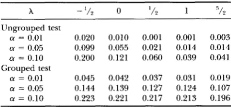
Power comparison between grouped and ungrouped tests

X - '/2 0 ' 1 2 1 5 / 2

Ungrouped test

a = 0.01 0.020 0.010 0.001 0.001 0.003

a = 0.05 0.099 0.055 0.021 0.014 0.014 a = 0.10 0.200 0.121 0.060 0.039 0.041

a = 0.01 0.045 0.042 0.037 0.031 0.019 a = 0.05 0.144 0.139 0.127 0.124 0.107 a = 0.10 0.223 0.221 0.217 0.213 0.196

Grouped test

Simulated data are generated from the Cx( C O ) ~ model then

tested against the hypothesis that the data are from the Cx( Co)' model. Different X's correspond to different test statistics in power divergence family. a is the significance level at which the test is carried out.

model. The hypothesis model is used to fit the simulated data, and the Pvalue of the test statistic is calculated by the Monte Carlo approximation as described above. Two thousand such samples are generated, and the Pvalues are calculated. For a levela test we reject the null hypothesis if the calculated Pvalue is <a. The power of the test thus can be approximated by the per- centage of times that the null hypothesis is rejected. For each dataset several test statistics from the so-called

power divergence family

( R E A D

and CRESSIE 1988) are used. The test statistics in this family have the form

This family includes several well-known test statistics. For example, X = 1 gives Pearson's chi-square statistic, and X = 0 gives the log-likelihood ratio test statistic. For each sample each test is applied on both ungrouped and grouped classes. Grouping is done in such a way that all offspring types with more than three recombinations are put together to form a larger class, whereas the other types are kept separate. Two pairs of null and alternative hypotheses are considered. In both cases the null hypothesis is set to be the model Cx( Co)'. The alternative is Cx( Co) in the first pair and CxCo in the second pair. The results are summarized in Table 8 and Table 9.

(8)

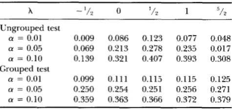
1052 H. Zhao, T. P. Speed

TABLE 9

Power comparison between grouped and ungrouped tests

x

0 l/2 1 :’/2

Ungrouped test

a = 0.01 0.009 0.086 0.123 0.077 0.048 a = 0.05 0.069 0.213 0.278 0.235 0.017

a = 0.10 0.139 0.321 0.407 0.393 0.308

a = 0.01 0.099 0.111 0.115 0.115 0.125 a = 0.05 0.250 0.254 0.251 0.256 0.271 a = 0.10 0.359 0.363 0.366 0.372 0.379

Simulated data are generated from the CxCo model then tested against the hypothesis that the data are from the

Cx( Co)‘ model. Grouped test

COMPARISON WITH THE MODEL OF GOLDGAR AND FAIN

A thorough comparison of different models is made by MCPEEK and SPEED ( 1995)

.

In this section we focus on the comparison of the C x ( Co) model with a model proposed by GOLDGAR and FAIN ( 1988). In that model, which is similar to the count-location model (KARLIN and LIBERMAN 1979 and RISCH and LANGE 1979), GOLDGAR and FAIN ( 1988) assume that the number of crossovers follows a distribution that has to be estimated from the data. Their model differs from the count-location model in two respects: (1) given the number of crossovers, their locations are not independent, but they follow a specified joint distribution in which some parameters have to be estimated; ( 2 ) instead of putting the distribution on the four-strand bundle, these distributions are put on the single meiotic product, i.e., it is a two-strand model. In fact, it is not possible to construct a four-strand NCI model that is consistent with their model on a single meiotic product (see D. GOLDSTEIN, H. ZHAO and T. P. SPEED unpublished results). In their paper GOLDGAR and FAIN show that their model fits data much better than the count-location model and several two-strand models based on map functions. Esti- mates of genetic distances among markers from WEINSTEIN’S and MORGAN’S data by their model

( GOLDGAR and FAIN 1988)

,

as well as the estimates based on the C x ( Co) model, are given in Table 10 and Table 11.

Besides genetic distances the parameters used by

TABLE

md M. S. McPeek

GOLDGAR and FAIN are as follows: d j , i = 0, 1, 2 and 3, the probabilities of 0 , 1 , 2 and 3 crossovers, respectively;

k , which measures the degree of interference, and q,,

the genetic distance between the centromere and the marker closest to it. So when n

+

1 markers are involved in the experiment, a total of n

+

5 parameters have to be estimated. On the other hand for the

Cx(

Co) ’”

model, n

+

1 parameters are used, including n genetic distances between each pair of consecutive markers and the parameter m that measures interference. Thus, in general, four fewer parameters are needed for the

C x ( Co)

‘‘

model than for GOI.DGAR and FAIN’S model. For some organisms it is reasonable to assume there are no more than three crossovers. For example, among 28,239 offspring in MORGAN’S D. melunoguster data, only two offspring showed recombination in four intervals at the same time, and no such individual was recorded in WEINSTEIN’S data. On the other hand for those organisms that have a large number of crossovers during meiosis, e.g., S . pombe, probabilities of 4, 5 or even more crossovers on the four-strand bundle must be estimated when GOLDGAR and FAIN’S model is used. One should also specify the joint distribution of these crossover locations. In this case the model loses its simplicity and credibility when many joint distributions must be assumed based on empirical observations.

A good model should both fit the data and be biologically reasonable. Recall that crossovers occur among four-chromatid strands, so under the assumption of no chromatid interference, we can relate the probabilities of crossover patterns on the four-strand bundle and those on a single strand. Under GOLDGAR and FAIN’S model when the probabilities of crossover patterns on a single strand are specified, some crossover patterns on the four-strand bundle will have negative probabilities under the assumption of NCI. Thus, the model they describe is incompatible with the assumption of NCI. We tried a variation of GOLDGAR and FAIN’S model in which we put the distribution on the four-strand bundle instead of on a single strand. Under the assumption of NCI, we derived the probability of each recombination pattern for single spore data. This slightly modified version of GOLDGAR and FAIN’S model fits the Drosophila data as well as the original one.

Coincidence curves: The traditional measure of in-

terference is coincidence ( STUKTEVANT 1915; MULLER

10

Comparison with GOLDGAR and FAIN’S model (WEINSTEIN’S data)

~

Interval sc-ec ec-cL, cv-ct ct-v v-g R-f LR

GOLDGAR and FAIN 7.2 9.9 8.6 15.0 11.4 11.4 132.4

C.x( Co) 7.1 9.6 8.3 14.8 11.5 11.5 219.1

(9)

TABLE 11

Comparison with GOLDGAR and FAIN’S model (MORGAN’S data)

Interval sc-ec ec-cv cv-ct ct-u V-S s-f f-ca ca-b LR

GOLDGAR and FAIN 5.2 10.1 7.8 13.5 8.3 15.7 7.3 4.5 159.5

Cx( CO) 5.1 9.8 7.5 13.3 8.4 15.6 7.5 4.4 174.8

Estimated genetic distances based on GOLDGAR and FAIN’S model and the CX(CO)~ model, together with likelihood ratio

statistics (LR).

1916), which is expressed as a ratio. The numerator is the chance of simultaneous recombination across both of two disjoint intervals on the chromosome. The de- nominator is the product of the marginal probabilities of recombination across the intervals.

TI 1

S =

( q n

+ ~ 1 1 )

’

where S is the coincidence and rq is the chance of i recombinations across the first interval and j recombinations across the second interval. The coincidence curve for a model is a plot of the coincidence against the genetic distance between two intervals, where the widths of the two intervals are taken to be infinitesimal. (Foss et al. call this quantity S4.) Foss et al. (1993) compare the coincidence curves ( S) for the Cx( Co) model with empirical coincidence curves estimated from data. They find that the theoretical curves are very close to the empirical ones. Similarly, we draw the S

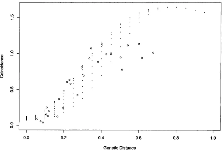
curves based on the modified version of GOLDGAR and FAIN’S model (Figure 1 )

.

In GOLDGAR and FAIN’S model

S is not only a function of the genetic distance between the two regions under study but also depends on how far these regions are from the centromere, so the S

curve cannot be uniquely drawn on the graph. Instead, for a given genetic distance between two regions, S can vary according to the distance to the centromere. It is clear from the graph that GOLDGAR and FAIN’S model predicts that Swill be >1.5 when the distance between the two regions is bigger than 60 cM, no matter where they are located on the chromosome. But this predic- tion is not consistent with the empirical results in which

S is always smaller than 1.2.

DISCUSSION

Based on the derived probabilities for each single spore or tetrad recombination pattern, we use the method of maximum likelihood to fit the

Cx(

Co) model to a variety of organisms. The estimated m’s

based on statistical analyses of D. melanogaster and N.

CTUSSU data agree with those given by Foss et al. ( 1993) ,

where m was estimated by the ratio of gene conversions

I I I I I - ~ T

0.0 0.2 0.4 0.6 0.8 1 .o

Genetic Distance

FIGURE 1.-Comparison between predicted and observed Svalues for GOLDGAR and FAIN’S model. The dots above any given

genetic distance represent the range of possible predicted S values, which vary according to location on the chromosome. 0,

(10)

1054 H. Zhao, T. P. Speed and M. S. McPeek

to crossovers in genetic experiments. In humans we are currently able to provide only a preliminary estimate of m , although we hope that more extensive human datasets will soon become available. Whereas some amount of positive interference is shown in the above organisms, it is not present in two other organisms we analyzed, S. pombe and A . nidulans.

The m estimated from different experiments using genes on different chromosomes within the same organism turn out to be rather similar. This implies that as a measure of interference, m does not change across different chromosomes, thus, the degree of interference might be determined by factors specific to each organism.

We have discussed how to interpret the goodnessof- fit test statistic appropriately after fitting a model to a multilocus dataset. In multilocus data because many single spore or tetrad recombination patterns have rather small expected numbers of observations, even in an experiment of moderate size, the

x'

approximation to goodness-of-fit statistics often fails. Two ways of avoiding this difficulty are proposed: ( 1 ) simulating the distribution of the test statistic by a Monte Carlo method or

( 2 )

grouping small classes into a larger class. Our simulation study shows that the tests based on grouped classes usually have larger power than the tests based on ungrouped classes.

Among the four-strand models considered here, the four-strand version of the model of GOLDGAR and FAIN

(1988) gave the smallest likelihood ratio statistics (see Table 10 and Table 11 ) , but considering that this model has four more parameters than the chi-square model, the difference in likelihood ratio statistics is not impres sive. The count-location model has two parameters more than the chi-square model, yet it performed worse. In comparing the

Cx(

Co) '' model with the count-location model and GOLDGAR and FAIN'S model, we consider that a good model should not only yield a small test statistic but should also be parsimonious ( i . e . , have few parameters), biologically reasonable and generalizable to many organisms. In these respects the

Cx(

Co) model seems superior. It has a biological basis and is computationally tractable. Because of its simple structure, it can be applied to a broad range of organisms.

Although the Cx ( Co) '' model discussed in this paper applies well to data of different organisms and gives some insight into the underlying crossover process, there is a lot of room left for improvement. First of all, the parameter m need not be restricted to be an integer, but when m is not an integer, there are no explicit expressions for the probabilities of single spore or tetrad recombination patterns. In this case M. S. MCPEEK

and T. P. SPEED (unpublished results) use a simulation method to estimate the parameters. Second, we might suspect that the amount of interference varies in different regions within the same chromosome. A local m

rather than a global m might be fitted in the model. Finally, for some organisms with a high proportion of

conversion data observed, we need to develop a model to include both gene conversions and crossovers. A

good model of this kind should help us understand more about the crossing-over process.

The no-interference model is widely used in human genome mapping. Although it has been shown by SPEED et al. ( 1992) that the no-interference model is asymptot- ically robust for gene ordering, we do lose some efficiency in ordering and in excluding a test locus when there is interference in the underlying crossover process. D. GOLDSTEIN, H. ZHAO and T. P. SPEED (unpublished results) study the loss in efficiency using the no- interference model when the actual crossover process follows the

Cx

( Co) model. They find that the number of gametes required for these tasks is 10-50% smaller for the Cx( Co) '" model than for the no interference model, depending on the degree of interference and the distances between the markers.

We thank Professor JAMES HAWK and Dr. PEI'ER MUNZ for kindly supplying the data. This work was supported by National Science Foundation grant DMS-9113527.

LITERATURE CITED

BAILEY, N. T. J., 1961 Introduction to the Muthematzcal lhemy of C h e t i c

Linkage. Oxford University Press, London.

BARRATT, R. W., D. NEWMEYER, D. D. PERKINS and L. GARNJOBST, 1954

Map construction in Neurospora rrmsa. Adv. Genet. 6: 1-93,

BOI.E-GOWDA, B. N.,D. D. PERKINsand W. N. STRICKIANI), I962 Cross- ing-over and interference in the centromere region of linkage group I of Neurospora. Genetics 47: 1243-1252.

COBBS, G., 1978 Renewal process approach to the theory of genetic linkage: case of no chromatid interference. Genetics 89: 563-

581.

Foss, E., R. LANm, F. W. STAHI. and C. M. STF.INREK(;, 1993 Chiasma interference as a fhction ofgenetic distance. Genetics 133: 681 -

691.

G o I . I x ; ~ , D. E., and P. R. FAIN, 1988 Models of multilocus recombination: nonrandomness in chiasma number and crossover posi- tions. Am. J. Hum. Genet. 43: 38-45.

HAI.DANE, J. B. S., 1919 The combination of linkage values, and the calculation of distances behveen the loci of linked factors. J .

Genet. 8: 299-309.

HAWIIORNE, D. C., and R. K. MORTIMEK, 1960 Chromosome mapping in Saccharomyces: centromere-linked genes. Genetics 45:

1085-1110.

HAWHORNE, D. C., and R. K. MORTIMER, 1968 Genetic mapping of nonsense suppressors in yeast. Genetics 60: 735-742.

KARLIN, S., and U. LIBERMAN, 1979 A natural class of multilocus recombination processes and related measure of crossover interference. Adv. Appl. Probdb. 11: 479-501.

KARI.IN, S., and U. LIBERMAN, 1983 Measuring interference in the chiasma renewal formation process. Adv. Appl. Prohab. 15: 471 -

487.

KOHIJ, J., H. HOTTIN(;ER, P. MUNZ, A. STMUSS and P. THURIAIIX,

1977 Genetic mapping in Schizosacchuromyces pombt by mitotic and meiotic analysis and induced haploidizdtion. Genetics 87:

471-489.

MATHER, R, 1935 Reduction and equational separation of the chromosomes in bivalent5 and multivalents. J. Genet. 30: 53-78.

MCINNIS, M. G., A. CHAKRAVARTI, J. BIASC:HAK, M. B. PETERSEN, V.

SHW rt aL, 1993 A linkage map of human chromosome 21: 43 PCR markers at average intenrals of 2.5 cM. Germmics 16:

562-571.

MCPEEK, M. S., and T. P. SPEED, 1995 Modeling interference in

genetic recombination. Genetics 139: 000-000.

(11)

investigations on the constitution of the germinal material in relation to heredity. Carnegie Instit. Washington 34: 284- 291.

MORTIMER, R. R, and D. C. HAWTHORNE, 1966 Genetic mapping in Saccharomyces. Genetics 53: 165-173.

MORTIMER, R. K , and D. C. HAWTHORNE, 1973 Genetic mapping in Saccharomyces N. Mapping of temperature-sensitive genes and use of disomic strains in localizing genes. Genetics 7 4 33- 54.

MLJI.I.ER, H. J., 1916 The mechanism of crossinguver. Am. Nat. 50:

193-434.

PERKINS, D. D., 1962 Crossing-over and interference in a multiply marked chromosome arm of Neurospora. Genetics 47: 1253-

1274.

PRESS, W. H., B. P. FLANNERY, S. A. TEUKoLsKYand W. T. VE'ITERLING,

1988 Numm'cal Recipes in C. Cambridge University Press, Cam-

bridge, UK

READ, T. R. C., and N. A. C. CRESSIE, 1988 Goodnessafrfit Statisticsfor Discrete Multivariate Data. Springer-Verlag, New York.

RISCFT, N., and K. LANCE, 1979 An alternative model of recombina-

tion and interference. Ann. Hum. Genet. 43: 61-70.

RISCH, N., and K LANGE, 1983 Statistical analysis of multilocus recombination. Biometrics 39: 949-963.

SNOW, R., 1979 Maximum likelihood estimation of linkage and interference from tetrad data. Genetics 92: 231-245.

SPEED, T. P., M. S. MCPEEK and S. N. EVANS, 1992 Robustness of

the no-interference model for ordering genetic markers. Proc. Natl. Acad. Sci. USA 89: 3103-3106.

STRICKIAND, W. N., 1958 An analysis of interference in Aspergillus nidulans. Proc. R. Soc. Lond. Ser. B 149: 82-101.

STRICKLAND, W. N., 1961 Tetrad analysis of short chromosome regions of Neurospora crussa. Genetics 46: 1125-1141.

STURTEVANT, A. H., 1915 The behavior of the chromosomes as stnd- ied through linkage. 2. Indukt. Abstammungs-Vererhngsgsl. 13: 234- 287.

WEINSTEIN, A,, 1936 The theory of multiple-strand crossing over.

Genetics 21: 155-199.

ZHAO, H., M. S. MCPEEK and T. P. SPEED, 1995 Statistical analysis of chromatid interference. Genetics 139: 1057-1065.

Communicating editor: B. S. WEIR

APPENDIX

Lemma: Under the Cx( Co) model the probability of kj crossovers between Jj and . I,,,

,

j = 1,

. . .

, n is

1

P

- l D k , ( y l ) D k ~ ( ~ ) . " D ~ ( ~ , ) l ' ,

where

p

= m

+

1, y, =

2p3

and D k ( y ) has i, j t h entry

Proof: We start with the simplest case when there are

only two markers. Because the C events are randomly distributed on the four-strand bundle and the number of C's follows the Poisson distribution with parameter, say y, the chance of s C's is e-yy'/ s!. 1 /pof these C's will resolve as crossover event, and under the assumption of no chromatid interference, each strand has chance

'/2 of being involved in each crossover. So on average

each strand has ~/2pcrossovers, given s Cevents. Recall that the genetic distance is defined to be the expected number of crossovers on a single strand, so the genetic distance x and the Poisson parameter y are related by x =

y / 2 p ,

i.e., y = 2px.

In the following discussion suppose markers fl, . J 2 ,

. . .

, I, are laid out from left to right, and the Cevents occur also from left to right. The Cx( Co) model as-

e-YyPk+l-z

/

( p k

+

j - 2) !.

sumes that the crossover intermediate ( C) events resolve in sequence like CxCoCo- * * CoCxCo-

- -

and that the process is stationary, so the first Cevent to the right of has an equal chance of resolving as any of the m

+

1 elements of Cx( Co) m . The occurrence of k cross-

overs between JI and J2 might be the result of

p'

possible situations, depending on the number of Co's before the first Cx to right of . Il and the number of Co's between . J2 and the nearest Cx left to it. The number can vary from 0 to

p

- 1. Therefore, the chance of

kl Cx's between l1 and J2 can be computed as

The case i = 1 corresponds to the situation where the leftmost C between . J1 and 1' is a Cx, and the rightmost C could be either one Cx

(pkl

-

p

+

1 C's altogether between II and J 2 ) , the first Co after a Cx (

pkl

-

p

+

2 C's) or the second Co after a Cx, etc. i - 1 corresponds to the number of Co's between l1 and the first Cx.

We can write the sum in a matrix product form:

Each element in the first column of the matrix corresponds to the last C event between I , and l2 being a Cx; the second column corresponds to the last C being the first Co after the k,th

Cx,

the j t h column to the j t h Cafter the klth Cx. Therefore, the sum of the j t h ( j

>

0 ) column multiplied by

l / p

is the probability that there are kl crossovers between . II and J p , and the last

C event is the ( j - 1 ) th Co after the k , th Cx. Therefore if we define

then

pi,

is the probability that the last C between I , and l2 is the ( j - 1 ) th Co after the k , th Cx with the exception that

$I:,

is the probability of the last C being the klth Cx.

Now we consider the case for three markers . I ] , l2 and . Is. Given that the first Cto the right of l2 is the lth Co after a Cx, the probability of h2 crossovers between J,

and J3 is

(12)

1056 H. Zhao, T. P. Speed and M. S. McPeek

which is

p$,"'.

Therefore the chance of k1 crossovers between 1 1 , .,f2, and

k2

crossovers between l2 and

13 is

Rewriting the above relation in matrix form, we get

Recall that

(Pil

92,

*

- -

Pg,)

= ( 1 1 * * 1 )

Dk, ( y l )

,

thus the probability of kl crossovers between

f l and . fB, k2 crossovers between . l2 and . f3 is

l D k ~ ( y l ) D l c ~ ( y Z ) l ' .

The general result involving ?z intervals can be proved

Theorem 1: Define by the same method.

Nj = Do(.~j)

+

' / 2

C

Ds(y1) 7

7 2 1

Rj ==

'12

C

Ds(yj) 9

s z 1

then the probability of recombination pattern ( i l i 2 . * in) is

1

P ( i l i 2 .

.

* i n ) = - 1MLM2. * .M,,l',

P

where Mj = Nj when

4

= 0 , and Mj =

Rj

when

4

= 1. Proof: It is well known that given k 2 1 crossovers

between two markers, the chance of a recombination on a single strand is 1/2, and there can be no recombination if no crossovers occur. We can write

Phk)

for the probability of no recombination and $I$') for the probability of recombination given k crossovers occurring. So

pho)

= 1,

p i o )

= 0 and

p j k )

=

$ik)

= when k 2 1. Write P'(~;$:..injk~~) for the probability of observing recombination pattern ( i l i 2

- -

* in) when there are

kj

crossovers in the jth interval, j = 1, 2,

.

, n. Then we have

x

Dk2(p>) a ' p!,".'Dk,(yn) 1 '

k,

1

P

= - lMlM2. .Mnl I .

Theorem

2:

Define

Pj = D O ( J ~ )

+

C

' / 3 ( ' / 2

+

( - 1 / 2 ) k ) D s ( ~ J ) S 2 2

Tj = Dl(rj)

+

C

' / 3 ( 1 - (-1/2)k)Ds(ylJi)

5 2 2

Nj =

C

' / ~ ( ~ / 2

+

( - ' / ~ ) ~ ) D s ( y j ) .

,= 2

Then the probability of tetrad pattern ( i l i 2

-

*

-

2 % )

can be written as

1

P ( i l i 2 ' * i n ) = - 1MIM2. * M n l ' ,

P

where Mj = Pj if il = 0 , Mj = Tj if zi = 1, and Mj = Nj

if

4

= 2.

Proof: Notice that given k 2 1 crossovers between two markers, the probabilities of parental ditype, tetratype and nonparental ditype are '/3 ( ' / 2

+

( - '1'2) ') ,

*/3 ( 1 - ( - ') and ( 1/2

+

( - 1/2) k ) , respectively.