A Tabu Search Approach to Multiple Sequence Alignment

ABSTRACT

LIGHTNER, CARIN ANN. A Tabu Search Approach to Multiple Sequence Alignment.

(Under the direction of Dr. Shu-Cherng Fang.)

Sequence alignment methods are used to detect and quantify similarities between

different DNA and protein sequences that may have evolved from a common ancestor.

Effective sequence alignment methodologies also provide insight into the structure\

function of a sequence and are the first step in constructing evolutionary trees. In this

dissertation, we use a tabu search approach to multiple sequence alignment. A tabu

search is a heuristic approach that uses adaptive memory features to align multiple

sequences. The adaptive memory feature, a tabu list, helps the search process avoid local

optimal solutions and explores the solution space in an efficient manner. We develop two

main tabu searches that progressively align sequences. A randomly generated bifurcating

tree guides the alignment. The objective is to optimize the alignment score using either

the sum of pairs or parsimony scoring function. The use of a parsimony scoring function

provides insight into the homology between sequences in the alignment. We also explore

iterative refinement techniques such as a hidden Markov model and an intensification

heuristic to further improve the alignment. Moreover, a new approach to multiple

A Tabu Search Approach to Multiple Sequence Alignment

by

Carin Ann Lightner

A dissertation submitted to the Graduate Faculty of

North Carolina State University

in partial fulfillment of the

requirements for the Degree of

Doctor of Philosophy

Operations Research

Raleigh, North Carolina

2008

APPROVED BY:

______________________________ ______________________________

Dr. Shu-Cherng Fang Dr. Henry L. W. Nuttle

Chair of Advisory Committee

______________________________ ______________________________

Dr. Elmor Peterson Dr. Simon M. Hsiang

Dedication

This dissertation is dedicated to my mother, Patricia Ann Lightner. Although she is only

still here with us in spirit, so much of who I am has been shaped by her love,

encouragement, understanding, support and selflessness. She was given the arduous task

of raising three young women. With grace, poise and determination, she showed me how

to be a better person and what it truly means to sacrifice everything for someone else’s

benefit. So, I would like to express my sincere gratitude for everything she has instilled

in me and dedicate this dissertation to her loving memory.

Biography

Carin Ann Lightner was born April 25, 1977 in Cleveland, Ohio to her parents

Patricia and Ardie Lightner. She is the youngest of her two siblings, Constance and

Cynthia. In 1995, Carin graduated from Hathaway Brown School in Shaker Heights,

Ohio.

Carin began her collegiate studies at Norfolk State University (NSU) as a

Dozoretz National Institute for Mathematics and Applied Sciences (DNIMAS) scholar in

the summer of 1995. After 3 ½ years in the Mathematics department at NSU, she

transferred to North Carolina Central University, where she obtained a B. S. degree in

Mathematics in December 1999.

Carin began her graduate studies in the Operations Research program at North

Carolina State University (NCSU) as a David and Lucille Packard Fellow in the spring of

2000. She obtained an M.O.R. degree in August 2002 and continued in the graduate

program as a Ph. D. student. She began working with Dr. Shu-Cherng Fang as her Ph. D.

thesis advisor and pursued her research interests in the area of Bioinformatics and Soft

Computing. After years of rigorous studies, she looks forward to future endeavors and

pursing a career in academia.

Acknowledgments

I would like to thank my two sisters, Constance and Cynthia Lightner. As the

youngest, I have often walked in their footsteps and have been guided at various

junctures of my life by their words of encouragement and advice. I am so appreciative

that they opened up many doors for me and helped make my path a little easier.

I would like to express my gratitude and sincere thanks to Dr. Shu-Cherng Fang.

I have learned a great deal from him that extends far beyond the realms of academia. He

has been extremely patient and understanding, throughout a long yet rewarding journey

through NCSU. For his knowledge and wisdom, he has truly been an outstanding advisor

and mentor.

A special thanks to Dr. Nuttle, Dr. Peterson and Dr. Hsiang for being on my

advisory committee. I have benefited from their time, revisions and expertise.

The faculty at NCSU has been integral in my maturation as a student. I am

appreciative of their instruction and superb guidance.

I am grateful to have been a part of the FANGroup. I would like to thank

everyone for their help and encouragement throughout my studies.

Table of

Contents

List of Tables . . . viii

List of Figures . . . x

1 Introduction . . . 1

1.1 Basics about Nucleic Acids and Genetic Sequencing . . . 1

1.1.1 Nucleic Acids . . . 1

1.1.2 DNA Sequencing . . . 2

1.1.3 Dynamic Programming Approach . . . 3

1.2 Multiple Sequence Alignment . . . 9

1.2.1 General Approach . . . 9

1.2.2 Scoring an MSA . . . 11

2 Literature Review . . . 14

3 New Approach to Multiple Sequence Alignment . . . 23

3.1 Overview . . . 23

3.2 Use of Tabu Search vs. Other Sequence Alignment Algorithms . . . 24

3.4 Tabu Search A and B . . . 27

3.5 Hidden Markov Model for Local Improvement of MSA . . . 31 3.5.1 Basics Components of HMM . . . 31

3.5.2 Forward and Backward Algorithms . . . 33 3.5.3 Viterbi Algorithm . . . 34

3.5.4 Expectation Maximization Method . . . 36

3.6 Modified Tabu Search: Tabu A’ . . . 38

3.7 Summary . . . 40

4 Computational Experiments for Tabu A, B and A’ . . . 42

4.1 Overview . . . 42

4.2 Sequence Generation and Experimental Cases . . . 42

4.3 Tabu B vs. Other MSA Programs . . . 44

4.3.1 Alignment Score . . . 44

4.3.2 CPU Time . . . 47

4.3.3 Tabu B with HMM Local Improvement Algorithm vs. SAGA . . . 49

4.4 Tabu A vs. Tabu B . . . 55

4.5 Tabu A vs. Tabu A’ . . . 57

4.6 Summary . . . 60

5 Improved Tabu Search: Tabu C . . . 64

5.1 Overview . . . 64

5.2 Components of Tabu C . . . 64

5.2.1 Solution Representation . . . 64

5.2.3 Intensification/ Diversification Components . . . 70

5.2.4 Scoring an MSA . . . 71

5.3 Modifications to the DP Algorithm . . . 73 5.4 Summary . . . 76

6 Computational Experiments for Tabu B, C and A’ . . . 77

6.1 Overview . . . 77 6.2 Sequence Generation and Experimental Cases . . . 77

6.3 SP Scoring Method . . . 78

6.3.1 Tabu B, C, A’ vs. Other MSA Programs . . . 78 6.4 Parsimony Scoring Method . . . 85

6.5 CPU Time . . . 85

6.6 Summary . . . 89

List of Tables

Table 4.1 Details about thefirst four experimental cases . . . 44

Table 4.2 SP alignment scores from ClustalW, SAGA, PRALINE and Tabu B . 46

Table 4.3 Measures for the 10 tabu search runs per group using Tabu B . . . 47

Table 4.4 Average CPU times from ClustalW, SAGA, PRALINE and Tabu B . 50

Table 4.5 CPU time measures for Tabu B . . . . 51

Table 4.6 Improvement in MSA score for Tabu B with HMM . . . 54

Table 4.7 MSA scores for the Tabu B with HMM and SAGA . . . 54

Table 4.8 Measures for the 10 tabu search runs per group using Tabu B + HMM 55

Table 4.9 Percentage Improvement in CPU times between Tabu A andTabu B . 59

Table 4.10 SP scores from Tabu A and Tabu A’ . . . 61

Table 4.11 Measures for 10 tabu search runs per group using Tabu Aor Tabu A . 62

Table 6.1 Details about experimental cases 5 and 6 . . . 78

Table 6.2 SP scores from ClustalW, KALIGN, PRALINE and PRRN . . . 80

Table 6.3 SP scores from SAGA, Tabu B, Tabu C and Tabu A’ . . . 81

Table 6.4 Measures for the 10 tabu search runs per group using Tabu B, Tabu C

Table 6.5 Measures for the 10 tabu search runs per group using Tabu B, Tabu C

and Tabu A’ (Groups with 40-80 sequences) . . . . . . . .. 83

Table 6.6 Parsimony scores for ClustalW and Tabu C . . . 86

Table 6.7 Measures for the 10 tabu search runs per group using Tabu C . . . . 87

Table 6.8 CPU time from ClustalW, KALIGN, PRALINE and PRRN . . . 90

Table 6.9 CPU time from SAGA, Tabu B, Tabu C and Tabu A’ . . . 91

Table 6.10 CPU time measures for Tabu B, Tabu C and Tabu A’ (Groups contain

10-40 sequences ) . . . . 92

Table 6.11 CPU time measures for Tabu B, Tabu C and Tabu A’ (Groups

List of Figures

Figure 1-1 Sequences evolve through a combination of mutations . . . 3

Figure 1-2 Pairwise and multiple sequence alignment . . . 4

Figure 1-3 Basic idea behind DP approach . . . 4

Figure 1-4 A sequence alignment can end in one of three ways . . . 5

Figure 1-5 Illustration of Needleman and Wunsch’s DP approach . . . 6

Figure 1-6 Example of Gotoh’s DP algorithm . . . 8

Figure 1-7 An example of multiple sequence alignment . . . 10

Figure 1-8 Calculation of SP score . . . 11

Figure 3-1 Illustration of neighbor selection in a tabu search . . . 25

Figure 3-2 Procedure for basic tabu search . . . 26

Figure 3-3 Illustration of pairwise and block moves . . . 28

Figure 3-4 An example of a solution for Tabu A. . . 30

Figure 3-5 Hidden markov model for multiple sequence alignment . . . 32

Figure 3-6 An example of calculations from the foward and Viterbi algorithms . . 35

Figure 4-1 CPU time vs. Sequence length in MSAs with 20 sequences . . . 51

Figure 4-3 CPU time vs. Number of sequences in an MSA (with 18-21 BP) . . . 52

Figure 4-4 CPU time vs. Number of sequences in an MSA(with 150-201 BP) . . 53

Figure 4-5 Time complexity for DP algorithms . . . 56

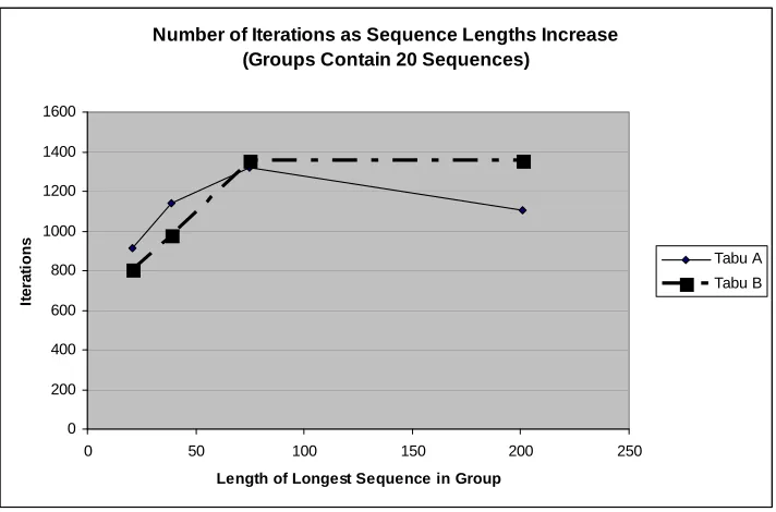
Figure 4-6 Iterations vs. Sequence lengths in MSAs with 20 sequences . . . 57

Figure 4-7 Iterations vs. Sequence lengths in MSAs with 200 sequences . . . 58

Figure 4-8 Iterations vs. Number of sequences in an MSA (with 18-21 BP) . . . . 58

Figure 4-9 Iterations vs. Number.of sequences in an MSA (with 150-201 BP) . . 59

Figure 5-1 Process of generating bifurcating tree and solution representation . . . 67

Figure 5-2 Possible moves to create a neighbor from an initial solution . . . 68

Figure 5-3 Additional moves to create neighbor from initial solution . . . 69

Figure 5-4 Parsimony score calculations using Fitch’s algorithm . . . 74

Figure 5-5 SP calculations for two MSAs with the same parsimony score. . . 75

Figure 6-1 Comparison of MSA scores for ClustalW, SAGA and Tabu C . . . 84

Figure 6-2 Comparison of MSA scores for Tabu B, Tabu C and Tabu A’ . . . 84

Chapter 1

Introduction

1.1

Basics about Nucleic Acids and Genetic Sequencing

1.1.1

Nucleic Acids

damaged [1]. The genetic information stored by DNA is transferred to RNA for protein synthesis. Protein synthesis is important because it accomplishes most of the functions of living cells such as catalyzing chemical reactions, providing structural support and helping protect the immune system. An organism’s genome contains its complete set of DNA. The arrangement of bases within the genome spells out specific instructions about an organism. These instructions spell out the way an organism looks, the organs it has, as well as all its biological components. In 2003, the human genome was sequenced with 3 billion base pairs. However, although the sequencing is known, there is still uncertainty with regard to the exact instructions spelled out for various subsequences within the human genome. To clear up some of the uncertainty about the genetic information within the human genome, researchers have used DNA sequencing. Researchers have discovered that DNA sequences of different organisms are often related. Also, similar genes are often conserved across divergent species and commonly perform similar or even identical functions. Thus, through sequence alignment of genes from various species, sequence patterns may be analyzed [27]. In general, DNA sequencing provides insight into the physical characteristics of an organism, the functions of proteins, the origins of diseases and possible cures for ailments.

1.1.2

DNA Sequencing

ances-A T C T C G ances-A G A T C - C C G A G A T C C G A G A T C C C G A G

Substitution Ancestral Sequence

Insertion Deletion

Figure 1-1: Sequences evolve through a combination of mutations

tor. Sequence alignment gives insight into the structure and function of a sequence, shows a common ancestry or homology between sequences, detects mutations in DNA that lead to genetic disease and is the first step in constructing phylogenetic or evolutionary trees.

Sequence alignment (SA) is an optimal way of inserting dashes into sequences in order to minimize (or maximize) a specified scoring function [1, 38]. Generally, genetic sequencing can be classified as a pairwise sequence alignment or a multiple sequence alignment (MSA). As displayed in Figure 1-2, MSA is simply an extension of pairwise alignments that align 3 or more sequences. Both MSA and pairwise SA can further be categorized as global or local methods. Where as global methods attempt to align entire sequences, local methods only align conserved regions of similarity.

1.1.3

Dynamic Programming Approach

S1 A T C T C G A G A S1 A T - C T C - G A G A

S2 A T C C - G A G A S2 A T - C C - G - A G A

S3 A T G T C G A C - G A

S4 A T G T C G A C A G A

S5 A T - - T C A A C G A

S1 A T C T - C G A G A S1 A T - C T C - - G A G A

S2 A T C C - G - A G A S2 A T - C C - G - - A G A

S3 A T - G T C G A - C G A

S4 A T - G T C G A C A G A

S5 A T - - T C A A - C G A

Infeasible Alignment Feasible Alignment

Infeasible Alignment

Feasible Alignment

Multiple Sequence Alignment Pairwise Sequence Alignment

Figure 1-2: Pairwise and multiple sequence alignment

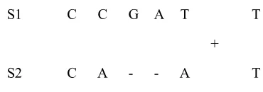
pair alone. Thus, if the scoring system is additive, the score for this alignment is the sum of the scores of thefirst five bases plus the score for aligning the last pair of bases.

In a pairwise sequence alignment, Figure 1-4 illustrates that for the ith _{base of sequence}

one,xi, and thejthbase of sequence 2,yj, there are only three waysxi andyj can be aligned;

eitherxiis aligned with yj, which gives a match or mismatch, xi is aligned with a gap oryj

is aligned with a gap [38]. In order to calculate the optimal cumulative score, S(i, j), we

S T A -A C S2 T + T A G C C S1

Sequence alignment broken into two parts T A -A C S2 T + T A G C C S1

xi xi xi

S1 C C G A T T S1 C C G A T T S1 C C G A T T

-S2 C A - - A T S2 C A - A T - S2 C A - - - A T

yj yj yj

aligned with a gap aligned with a gap

a.) Two bases aligned b.) Base in sequence 1 is c.) Base in sequence 2 is

Figure 1-4: A sequence alignment can end in one of three ways

must rely on the recursive and additive nature of the DP approach. The optimal cumulative score at bases xi and yj is:

S(i, j) = max

⎧ ⎪ ⎪ ⎪ ⎪ ⎪ ⎪ ⎪ ⎨ ⎪ ⎪ ⎪ ⎪ ⎪ ⎪ ⎪ ⎩

S(i₋1, j₋1) +s(xi, yj)

S(i₋1, j)₋d S(i, j₋1)₋d

where s(xi, yj) is the score for matching symbols xi and yj and d is the penalty for

introducing a gap.

Calculating the optimal cumulative score for the DP approach is best illustrated using an example adapted from Needleman and Wunsch’s paper. We calculate the optimal score using the array displayed in Figure 1-5a). Specifically, tofind an optimal sequence alignment of sequences CCGATT and CAAT, we can create an array, displayed in Figure 1-5b), with

five rows and seven columns. In this example, let the gap penalty, d, the match score and mismatch score equal 5, 1 and 0, respectively. For thefirst row, assign a score equal to(₋id)

for each cell(i,0). Similarly, for thefirst column, assign a score equal to(₋jd)for each cell

Figure 1-5: Illustration of Needleman and Wunsch’s DP approach

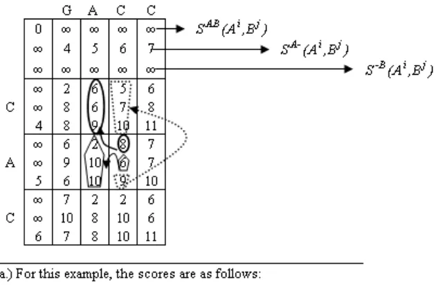
The example above has a scoring scheme that does not take into account differing penal-ties for opening a gap and extending a gap. When examining the evolution of sequences, opening up a gap is much more costly than extending an existing one. Gotoh’s algorithm [16] is a DP algorithm for global pairwise alignment that uses a linear gap penalty. A gap of lengthkis penalizeda+bk, whereais the gap open penalty and bis the gap continuation penalty. An array representation similar to the one presented above for the Needleman and Wunsch DP approach can be used for Gotoh’s algorithm. The difference is that Gotoh’s algorithm has three entries per cell instead of just one. For this approach, let thefirst entry in a cell,SAB(Ai, Bj),be the penalty associated with the best alignment between sequences

Ai _{and B}j _{that ends by pairing bases A}

i and Bj; let the second entry, SA−(Ai, Bj), be

the penalty associated with the best alignment between sequences Ai and Bj that ends by pairingAi with a gap;finally, let the third cell entry,S−B(Ai, Bj),be the penalty associated

with the best alignment between Ai and Bj that ends by pairingBj with a gap. Also, let

s(Ai, Bj)be the cost/score for aligning basesAi andBj. Recursive formulas forSAB(Ai, Bj),

SAB(Ai, Bj) = min_{SAB(Ai−1, Bj−1),SA−(Ai−1, Bj−1),S−B(Ai−1, Bj−1)_} +s(Ai, Bj)

SA−_(Ai_{, B}j_{) = min{S}AB_(Ai−1_{, B}j_{) +a,S}A−_(Ai−1_{, B}j_),S−B_(Ai−1_{, B}j_+a)}+b

S−B(Ai, Bj) = min_{SAB(Ai, Bj−1) +a,SA−(Ai, Bj−1) +a,S−B(Ai, Bj−1)_}+b

The score of the best alignment is the minimum of SAB(Ai, Bj), SA−(Ai, Bj) and

S−B(Ai, Bj) or simply the minimum of the values in the cell that is in the bottom right corner. The same trace back procedure in Needleman and Wunsch’s DP algorithm can be used here to recover the optimal alignment.

Sequences GACC and CAC are aligned in Figure 1-6a) using Gotoh’s algorithm[43] . In this example, the match, mismatch, gap open and gap extension scores are 0, 2, 3 and 1, respectively. The three values in cell (3,4),8,6, and9, are calculated using the surrounding cells in Figure 1-6a). The first entry, 8,is calculated using cell (2,3) and more specifically,

8=min_{6,6,9_}+ 2. The second entry, 6, is calculated using cell (3,3) and specifically,

6=min_{2 + 4,10 + 1,10 + 4_}. Finally, the third entry, 9, is calculated using cell (2,4) and specifically, 9=min_{5 + 4,7 + 4,10 + 1_}. In this alignment, the optimal score of 6 is found by taking the minimum value of the entries in cell (4,5). There are two optimal sequence alignments displayed in Figure 1-6b).

1.2

Multiple Sequence Alignment

1.2.1

General Approach

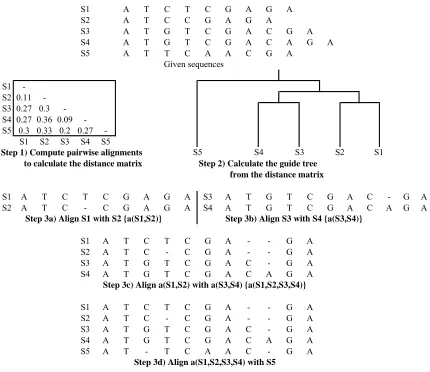
Multiple sequence alignments are often classified as progressive or iterative. Typically progressive alignments involve three steps. In the first step, each pair of sequences are aligned using the DP approach. Then, the scores from the pairwise alignments in step one are used to construct a tree. Finally, the tree from step two is used to progressively align the sequences and calculate an alignment score. In progressive algorithms, once a gap is introduced in the early stages of an MSA it is always present; thus one major drawback is that an error in an initial subalignment will be propagated throughout the entire MSA [27]. To avoid these problems, iterative techniques are used and initial alignments are constantly modified. An example of a progressive MSA is shown in Figure 1-7 [19]. The array in step one has all ten pairwise distance scores. A guide tree is constructed in step two following the distance matrix. In steps 3a)and 3b), sequences one andtwo are aligned, then sequences three and four are aligned. Next, the two subalignments from steps 3a)and 3b) are aligned. In the last step, sequencefive is aligned with the other four sequences and thefinal multiple sequence alignment is given.

S1 A T C T C G A G A

S2 A T C C G A G A

S3 A T G T C G A C G A

S4 A T G T C G A C A G A

S5 A T T C A A C G A

S1

-S2 0.11

-S3 0.27 0.3

-S4 0.27 0.36 0.09

-S5 0.3 0.33 0.2 0.27

-S1 S2 S3 S4 S5

S1 A T C T C G A G A S3 A T G T C G A C - G A

S2 A T C - C G A G A S4 A T G T C G A C A G A

S1 A T C T C G A - - G A

S2 A T C - C G A - - G A

S3 A T G T C G A C - G A

S4 A T G T C G A C A G A

S1 A T C T C G A - - G A

S2 A T C - C G A - - G A

S3 A T G T C G A C - G A

S4 A T G T C G A C A G A

S5 A T - T C A A C - G A

Step 3c) Align a(S1,S2) with a(S3,S4) {a(S1,S2,S3,S4)}

Step 3d) Align a(S1,S2,S3,S4) with S5

Step 3b) Align S3 with S4 {a(S3,S4)}

Given sequences

Step 1) Compute pairwise alignments to calculate the distance matrix

S5 S4 S3 S1

Step 2) Calculate the guide tree from the distance matrix

Step 3a) Align S1 with S2 {a(S1,S2)}

S2

Figure 1-7: An example of multiple sequence alignment

Figure 1-8: Calculation of SP score

1.2.2

Scoring an MSA

The sum of pairs (SP) method,first introduced by Carrillo and Lipman [6], is the simplest way to score an alignment. The SP score for an MSA with N sequences is defined as the sum of the scores of the N(N-1)/2 pairwise alignments For each column, this scoring scheme sums up the cost for every pair of bases as well as each gap and base pair. Then all column costs are summed to give the score for the alignment. The SP score is calculated for a multiple sequence alignment in Figure 1-8. Although the SP score is commonly used to score an MSA, there is not a biological or probabilistic justification for using this scoring scheme [9]. Also, this method tends to overestimate evolutionary events as the number of sequences increases [38, 2]. The sequences are scored as if they are not homologous and descendants of a common ancestor. Instead each sequence is scored as if it is a descendant of the others. To balance the overestimation problem, a weighted sum of pairs score is often used [9].

problem between sequences p and q in the SP score. Also, s(mpj, mqj) is the substitution

scoring function that gives the score for aligning nucleotides pj and qj in column j. The

formulation of the weighted SP score for an MSA is as follows:

w(M SA) = P

1≤p<q≤k

Ã

αp,q∗ L

P

j=1

s(mpj, mqj)

!

There are various weighting schemes and substitution scoring functions that are used to calculate a weighted SP score. Other scoring methods include a star phylogeny, information content and graph based trace methods [27]. In general, because there is not a standard scoring scheme for multiple sequence alignments, different scoring schemes will affect and alter the final alignment. Many of the existing MSA programs use a variety of scoring functions. In Chapter 2, there is a review of commonly used MSA programs and the corresponding scoring functions.

In Chapter3, we introduce a tabu search approach to multiple sequence alignment. Three tabu searches are implemented that attempt to maximize the SP scoring function. We start with an initial tabu search, Tabu A. The initial tabu is modified by implementing two subsequent tabu searches, Tabu B and Tabu A’, to improve either the CPU time or SP score of Tabu A.

In Chapter 4, we present the computational results from using Tabu A, Tabu B and Tabu A’ to align multiple sequences. We examine the MSAs, SP scores and CPU times generated from each of the tabu searches for several groups of sequences. ClustalW, PRALINE and SAGA are used to align the same groups of sequences. The results from these other MSA programs are compared with the results from the tabu searches.

parsimony score is used to evaluate the alignments. Additional components are also added to Tabu C to help locally improve the MSAs.

In Chapter 6, we present the computational results from Tabu B, Tabu C and Tabu A’ to align multiple sequence. The alignment scores and CPU times from the three tabu searches are compared with the results from ClustalW, KALIGN, PRALINE, SAGA and PRRN.

Chapter 2

Literature Review

ClustalW is a commonly used multiple sequence alignment program [20, 42, 21]. As with any other heuristic, ClustalW does not guarantee an optimal solution. It progressively aligns sequences and exploits the fact that similar sequences are evolutionarily related. First, ClustalW aligns and scores all possible pairs of sequences to determine their distance score. Then a guide tree is constructed using the edit distances and a neighbor joining algorithm. Finally, the guide tree is used to progressively align the sequences. Although an optimal solution is not guaranteed, ClustalW usually provides a good starting point for other

select-ing the parameters, ClustalW is most useful when sequences are known to be evolutionarily related.

Notredame and Higgins [30] have the best known genetic algorithm, Sequence Alignment by Genetic Algorithm (SAGA), for multiple sequence alignment. Similar to other genetic algorithms (GA), SAGA uses the principles of evolution to find the optimal alignment for multiple sequences. This method generates many different alignments by rearrangements that simulate gap insertion and recombination events to generate higher and higher scores for the MSA [27]. In this GA, the population consists of alignments that were formed from a complex set of twenty two different crossover and mutation operations. To determine the

fitness of an alignment, SAGA uses a weighted sum of pairs approach in which each pair of sequences is aligned and scored; then the scores from all the pairwise alignments are summed to produce an alignment score. As with any heuristic approach, SAGA may not generate an optimal MSA. Although it has been shown that SAGA does produce quality alignments, the time complexity involved in the weighted sum of pairsfitness function is a major drawback to this approach.

an optimal consensus sequence. This consensus sequence is simply a compact formulation representing all possible alignments for virtually any given number of sequences. With this GA, the total number of iterations needed tofind an optimal solution is independent of the number of sequences being aligned but dependent on the length of the sequences.

Riaz et al. [34] propose a tabu search algorithm for multiple sequence alignment. The algorithm implements the adaptive memory features typical of tabu searches to align multiple sequences. Both aligned and unaligned initial alignments/solutions are used as starting points for this algorithm. Aligned initial solutions are generated using Feng and Doolittle’s progressive alignment algorithm [11]. Unaligned initial solutions are formed by inserting a fixed number of gaps into sequences at regular intervals. The quality of an alignment is measured by the COFFEE objective function [31]. In order to move from one solution to another, the algorithm moves gaps around within a single sequence and performs block moves. This tabu search uses a recency-based memory structure. Thus, after gaps are moved, the tabu list is updated to avoid cycling and getting trapped in a local solution. This tabu search has two parts. Thefirst part of the algorithm implements a typical tabu search procedure, outlined in the next chapter, until the solution or an alignment is stabilized. Then the second part of the algorithm uses a intensification and diversification procedure, which focuses on poorly aligned regions. Finally, the algorithm terminates when no more poorly aligned regions are identifiable and the alignment quality cannot be improved. As with any heuristic approach, an optimal solution is not guaranteed; however generally, this tabu search produces comparable results to ClustalW and various other alignment programs. Lukashinet al. [25] propose a simulated annealing (SA) approach to multiple sequence alignment. This procedure is based on the Metropolis-Monte Carlo algorithm. The

function. The multiple sequence alignment problem for N sequences attempts to find the alignment that maximizes the cost function or matching score

M(s) =PL

k+1

N_P−1

i=1

N

P

j=i+1

Comp(Si(k), Sj(k))− N

P

i=1

P(Si)

where L is the new length of the aligned sequence, iand j represent the sequence num-ber, k represents the base position, P(Si) is the gap penalty function and the function

Comp(Si(k), Sj(k)) compares two bases from different sequences and reflects the degree of

similarity.

In general, the simulating annealing procedure starts offat a high temperature that allows many moves to alignments that have both better and worse scores. This feature, that allows moves to a worse scoring alignment, helps SA procedures avoid local optimal solutions. A cooling scheme is introduced to gradually decrease the temperature, the number of overall moves and the moves to worse scoring alignments. Eventually a global minimum is reached at the limit of zero-temperature. This algorithm was tested on E. Coli sequences and a consensus sequence of the aligned set was developed. One drawback of this algorithm is that the running time can vary tremendously depending on the selection of the cooling scheme and cost function.

rearrange-ment events. SLAGAN includes rearrangerearrange-ment events because DNA is known to mutate by simple edits, rearrangements such as translocations (a subsegment is removed and inserted in a different location but with the same orientation), inversions (a subsegment is removed from the sequence and then reinserted in the same location but with the opposite orientation) and duplications (a copy of a subsegment is inserted into the sequence and the original sub-sequence remains unchanged) or any combination of these simple edits. SLAGAN quickly aligns long sequences. In this technique, a penalty is incurred for the set of operations that include insertions, deletions, point mutations, inversions, translocations and duplications. This approach minimizes the sum of these penalties (edit distance). SLAGAN has three distinct stages. The first stage consists of finding local alignments using the CHAOS tool. The second stage picks the maximal scoring subset of the local alignments under certain gap penalties to form a 1-monotonic conservation map. Whereas standard global alignments are non-decreasing in both sequences, the structure of the 1-monotonic conservation map is non-decreasing in one sequence and without restrictions in the second sequence. Relaxing this assumption in the second sequence, allows the algorithm to detect rearrangements. The inclusion of rearrangement events is one of the features that makes this algorithm different than typical global alignment approaches. In the final stage of SLAGAN, the conservation map of local alignments is joined to form maximal consistent subsegments that are aligned using the LAGAN global aligner. One drawback of the SLAGAN algorithm is that it is not symmetric in the sequence order, so it frequently misses duplications in the sequences.

tree, called a suffix tree, that only stores the suffixes of a given sequence. The second stage

finds maximum unique matches between the sequences by traversing the suffix tree. A maximum unique match cannot be a subsequence of any longer such sequence and it must occur only once in both sequences. The third stage uses a variation of the longest increasing subsequence algorithm by putting the matches in the same order with respect to both se-quences. Thefinal stage uses a dynamic program to extract all locally optimal alignments in the non-matching regions and completes the global alignment. This algorithmfinds a near-optimal global alignment quickly. Also, this global pairwise method can be used in typical multiple sequence alignments to perform the initial pairwise comparisons. One drawback of this algorithm is that it only uses simple edits and does not permit rearrangements.

the three highest scoring diagonals quantifies the sequence similarity. This method is much faster than performing all pairwise alignments. Based upon this sequence similarity score, the UPGMA clustering method [40] is used to construct a guide tree. KALIGN follows the guide tree to progressively align the sequences using a dynamic programming algorithm.

PRRN is a global multiple sequence alignment program proposed by Gotoh [17]. PRRN is a best-first search iterative refinement strategy with tree-dependent partitioning for multiple sequence alignment. The main feature of the strategy is the iterative refinement stage. To make the alignment, phylogenetic tree and pair weights mutually consistent, a doubly-nested randomized iterative (DNR) method is used. The iterative refinement is based on a group-to-group sequence alignment (GSA) algorithm that uses an affine gap cost. In order to incorporate the piecewise linear gap cost into the GSA algorithm, the gap lengths are calculated. The true optimum may not be attained using the GSA algorithm since it is a hill-climbing heuristic. PRRN is most effective when refining an alignment that was obtained by an alternative progressive alignment method.

be done efficiently using the Pearch and Kelly online topological ordering algorithm (2004). Use of the Pearch and Kelly algorithm allows for rapidly constructed global multiple align-ments. In general, sequence annealing has the advantage that the intermediate alignments produced during the annealing process help identify locally conserved regions of similarity in the alignment.

BLAST [3] and variations of this algorithm are some of the most commonly used heuristic local alignment programs. These programs compare DNA/ protein sequences to DNA/protein databases in order tofind patches of regional similarity. Gapped BLAST attempts to opti-mize a similarity measure by searching the database in two phases. First, it uses a two-hit method that requires the existence of two non-overlapping segments, on the same diagonal within a specified distance. If these two word pairs each have an aligned score that is at least above a threshold parameter, T, then gap BLAST extends these subsequences. Finally, the algorithm uses dynamic programming to extend these two subsequences and only examines alignments that drop in score no more than a specified amount below the best score yet seen. Selecting the threshold parameter can be difficult because there is a trade-offbetween speed and sensitivity. While a higher value of T speeds up the search, it also has a lower probability of finding weak regional similarities. Generally, BLAST is most useful when there are compact highly conserved regions of similarity with sequence alignments.

Chapter 3

New Approach to Multiple

Sequence Alignment

3.1

Overview

HMM is only used to align 50 sequences or less. Thus, to improve the MSA score for larger groups of sequences, we implement Tabu A’. Tabu A’ is also a modified version of Tabu A.

3.2

Use of Tabu Search vs. Other Sequence Alignment

Algo-rithms

ClustalW, SAGA and most other MSA algorithms use a tree to guide the alignments. The guide tree is most commonly formed using both the distance scores and a neighbor joining algorithm. Sequences that are similar are clustered together in groups while dissimilar sequences are spread apart. The tree is used to form the MSA; then, both the tree and the MSA are used to determine phylogenetic relationships. The disadvantage to determining an MSA and predicting phylogenetic relationships based upon this type of guide tree is that tree does not attempt to minimize (or maximize) the most important measure of an MSA, the alignment score. Also, an incorrect guide tree might bias the results of an evolutionary tree used to predict phylogenetic relationships. Thus, we implement a tabu search approach based upon optimizing the sum of pairs scoring function of an MSA.

3.3

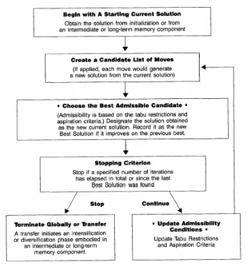
Basic Components of a Tabu Search

Some current solution

Generate neighboring solutions

Find best neighboring solution

Check if neighbor is accessible If not, select next best

neighbor

If yes, move to it and replace the current solution

Figure 3-1: Illustration of neighbor selection in a tabu search

solution. Accessible solutions are either not on the tabu list or are on the tabu list but satisfy conditions which allow exceptions to the tabu [10]. Generally, the steps displayed in Figure 3-1 are repeated, until some termination criteria is met.

3.4

Tabu Search A and B

We initially develop and implement two tabu search algorithms, Tabu A and Tabu B. The basic components of a tabu search algorithm outlined in the previous section are used in these algorithms. A solution consists of arrays that contain the sequence order and the positions of the gaps in the corresponding MSA. The actual MSA is not stored in memory. The optimality criterion attempts to maximize the most important measure of an MSA -the alignment score. Thus, the quality of an alignment is measured using the final alignment score. Finally, the algorithm terminates after the current best solution has not improved for a specified number of iterations.

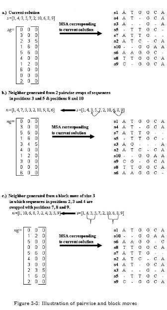
There are three types of move strategies that will generate a neighbor from a current solution. Using the solution representation from Tabu A, Figure 3-3 displays the first two types of moves. The first type of move is made by swapping pairs of sequences. In Figure 3-3a) the current solution, is composed of two arrays, s and sg, that contain the sequence order of the MSA and the gap locations, respectively. A possible neighbor, displayed in Figure 3-3b), is generated by swapping the sequences in positions 3 and 5 as well as the sequences in positions 8 and 10. For this neighbor, the arrays containing the sequence order and gap location are different from the arrays in the current solution. The second type of move is made by swapping blocks (two or more consecutive sequences) of sequences in particular positions. For example in Figure 3-3c), a possible neighbor of the current solution is generated by swapping sequences in positions 2, 3 and 4 with sequences in positions 7, 8 and 9. The third type of move is made by changing the gap positions within a sequence. So, the array containing the sequence order would remain the same and only the array with the gap positions would change.

both algorithms have similar components, the difference lies in there basic structure. Tabu A, simply progressively aligns allN sequences together in the order specified by a solution. For the MSA in Figure 3-3a),s1is aligned withs4to compose the subalignment,a(s1, s4). Next,

s3is aligned with the subalignmenta(s1, s4)to compose the subalignment,a(s1, s4, s3). This progressive alignment continues until the entire MSA,a(s1, s4, s3, s5, s7, s2, s10, s6, s8, s9),is composed. One difference between the two tabu searches is that the solution representation of Tabu A consists of two parts, while that of Tabu B consists of g+ 1 parts,whereg is the number of equal-sized ordered groups that theN sequences are divided into. In thefirst step of Tabu B, the array, s, containing the sequence order is divided into g equal-sized groups. Each of the ordered groups is progressively aligned (separately) and the gap locations for the g subalignments are stored in arrays sG1, ..., sGg. Then, all of the subalignments are

progressively aligned to make up the MSA, a(sG1, sG2, ..., sGg). Figure 3-4 displays the

3.5

Hidden Markov Model for Local Improvement of MSA

3.5.1

Basics Components of HMM

A hidden Markov model (HMM) is a doubly stochastic process in which the states are not directly observable (i.e. hidden). However, by using a Markov model of other states that are observable, the hidden states can be indirectly and probabilistically observed. Generally, a hidden Markov model is defined by the vector of initial state probabilities, the state transition matrix and the emission probability matrix. HMMs can be used to align multiple sequences. An advantage of using an HMM is that penalty values for opening a gap, extending a gap, scoring matches and mismatches are not used. Thus, the variability and sensitivity of alignments due to these cost parameters is not an issue with this type of model. The HMM is deeply rooted in statistics and it considers all possible combinations of matches, mismatches and gaps to generate an alignment of multiple sequences [27]. This model aligns sequences locally and is directly influenced by the initial alignment. Therefore, if this model is used in conjunction with a heuristic that initially aligns the set of sequences globally, an improved multiple sequence alignment may be determined.

match state insert state delete state transition probability

D1 D2 D3 D4 D5 D6 D7

I0 I1 I2 I3 I4 I5 I6 I7

BEG _{M1 M2 M3 M4 M5 M6 M7} END

Figure 3-5: Hidden markov model for multiple sequence alignment

aligned column. Each arc represents a transition probability between hidden states. Any path through this model that starts with the BEG state and ends with the END state, has a probability associated with it. Analysis of these probabilities and the relationship between the hidden states and aligned sequences allows three basic questions to be answered. The

first question is with what probability does a given HMM produce a given sequence? The next question is what path through the hidden states has the highest probability or is most probable? The final question is what are the parameters of an HMM that most probably underlie a given set of sequences. Each of these three questions can be answered using the forward-backward, Viterbi and EM algorithms which will be described in latter sections.

Given an observation sequence, O = (o1, o2,...,oT), and N hidden states, an HMM is

commonly defined by the following three parameters adapted from Rabiner and Juang[33]:

Π= (πi) vector of initial state probabilities

A= (aij) state transition matrix

E= (ej(ot)) emission (observation) probability matrix

probabilities of going from one hidden state to another and the emission probability matrix contains the probability that a base will actually be emitted, or shown, in a particular position in an alignment. The emission and state transition matrices do not change in time as the system evolves [33].

3.5.2

Forward and Backward Algorithms

The forward algorithm is a recursive algorithm that determines the probability that a given HMM emits a particular sequence. The forward algorithm sums up the probability of every possible path through the hidden states. The basic idea behind the forward algorithm is as follows:

Let

ft(i) = Pr(observation |hidden state isi)∗Pr(all paths to state iat timet)

= Pr(o1, o2,...,ot |hidden state isi)∗Pr(all paths to state iat time t)

Initialize at t= 1

f1(i) =ei(o)∗πi i∈[1...N]

Repeat recursion for hidden states t= 2tot=T₋1

ft+1(j) =ej(ot+1)∗

(

N

P

i=1

ft(i)aij

)

i, j_∈[1..N], t_∈[1, ..., T₋1]

Finally, the sum of all partial probabilities gives the probability that a given observation sequence produces a given HMM or

Pr(O_|HMM) = PN

i=1

fT(i)

An example of forward algorithm calculations for a portion of an HMM is displayed in Figure 3-6a). In this example, the observation sequence, O, is GTCG. The calculations for

ft+1(j)are only displayed for states IO , M1, D1 and I1.

forward algorithm computes probabilities from the initial column in an observation sequence to a certain time, t, the backward algorithm computes probabilities from a certain time, t, to the final column in an observation sequence. For the backward algorithm, we have the following structure:

Let

bt(i) = Pr(ot+1, ot+2,...,oT |hidden state isi)∗Pr(all paths to state iat timet)

Initialize at t=T

bT(i) = 1 i∈[1...N]

Repeat recursion for hidden states with t=T₋1tot= 1

bt(i) = N

P

j=1

aij∗ej(ot+1)∗bt+1(j) i, j∈[1...N], t∈[1, ..., T −1]

3.5.3

Viterbi Algorithm

The Viterbi algorithm [33, 45] determines the best path through the hidden states. The Viterbi and forward algorithms are very similar. Whereas the Viterbi algorithm finds the partial best path into each state by taking the path with the maximum probability, the forward algorithm sums up the probability of all paths into each state. The partial best path is defined as the sequence of hidden states which achieves the maximum probability. For the Viterbi algorithm, define δt(i) as the maximum probability of all paths ending at

state iat time t, and ψ_t(i) as the previous state on the partial best path. The basic idea behind the Viterbi algorithm is as follows:

Initialize at t= 1

δ1(i) =ei(o1)∗πi

ψ₁(i) = 0

= 0 .0 5

= 0 .0 0 4 5

=0 .0 5 ψ 1(IO )= 0

=0 .0 0 4 5 ψ 2(M 1 )= IO

= 0 .0 0 5 ψ 2(D 1 )= IO

= 0 .0 0 0 3 7 5 ψ 3(I1 )= D 1 = 0 .2 5 *m a x { 0 .0 0 4 5 * 0 .2 7 ,0 .0 0 5 * 0 .3 }

= 0 .2 5 *m a x{0 .0 0 1 2 1 5 ,0 .0 0 1 5 }

δ 3(I1 )= eI1(C )*m a x { δ2(M 1 )*αM 1 I1 ,δ2(D 1)*αD 1 I1} = 0 .2 5 * 0 .2

δ 2(M 1 )= eM 1(T )*m a x{ δ1(b e g)*αb e g M 1, δ1(IO )*αIO M 1} = 0 .1 *m a x{ 0 * 0 .7 , 0 .0 5 * 0 .9 ]

= 0 .0 0 0 6 7 8

=m a x{ 0 * 0 .1 ,0 .0 5 * 0 .1 }

δ 2(D 1 )=m a x{ δ1(b e g )*αb e g D 1 ,δ1(IO )*αIO D 1}

a .) C a lc u la tio n s u sin g fo r w a r d a lg o r ith m

= 0 .2 5 * 0 .2

= 0 .1 [0 * 0 .7 + 0 .0 5 * 0 .9 ]

f2(M 1 )= eM 1(T )[ f1(b e g)*αb e g M 1 + f1(IO )*αIO M 1]

b .) C a lc u la tio n s u sin g V ite r b i a lg o r ith m δ 0(b eg )=1

δ 1(IO )= eI0(G )* πIO f0(b eg )=1

f1(IO )= eI0(G )* πIO

f2(D 1 )= [ f1(b e g)*αb e g D 1+f1(IO )*αIO D 1] = [0 * 0 .1 + 0 .0 5 * 0 .1 ]

f3(I1 )= eI1(C )[ f2(M 1 )*αM 1 I1+f2(D 1)*αD 1 I1] = 0 .2 5 [0 .0 0 4 5 * 0 .2 7 + 0 .0 0 5 * 0 .3 ]

= 0 .0 0 5

D1 D2

I0 I1 I2

BEG M1 M2

0.1 0 .2 0. 1 0.7 0.4 0.9 0 .3 0.2 7 0.33 0 .5 _0.3 0.7

o1=G

o2=T

o₃=C

o4=G

eM1(A)=0.1

eM1(C)=0.3

e_M1(G)=0.4

eM1(T)=0.2

e_IK(o_t)=0.25 K ∀

δt(i) = max

1≤i≤N {δt−1(i)aij}∗ej(ot)

ψ_t(i) = arg max

1≤i≤N {δt−1(i)aij}

Finally, the best path probability and the last state in the best path determined at

t=T is

P r(best path)= max

1≤i≤N {δT(i)}

and

ψBEST_T = arg max

1≤i≤N {δT(i)}

In order determine the actual sequence of hidden states in the best path, use ψ_t(i) to

find the state which led to ψBEST_T and continue to follow it backwards in a similar manner until t= 1

An example of Viterbi algorithm calculations is displayed in Figure 3-6b).

3.5.4

Expectation Maximization Method

rela-tively unchanged from one iteration to the next. Usually, this process converges within 10 iterations. Finally, after training the HMM, the Viterbi algorithm is used to find the most likely path for each sequence. These most likely paths for each sequence are then used to construct an MSA.

More specifically, the procedure for the EM method is as follows:

1.) Determine the length of the HMM directly by using an initial alignment or through averaging the length of all sequences.

2.) Initialize the transition and emission probabilities by using prior information from an initial alignment.

3.) Train the model with a subset of the data sequences.

a.) Calculate ft(i) and bt(i) for each hidden state using the forward and backward

algorithms.

b.) Use the forward algorithm to calculatePr(O_|HMM).

c.) Expectation step

i.) Calculate the expected number of times an observation, Ot,is emitted

from state i

Ei(ot) = _Pr(ft_O(i_|)_{HM M}∗bt(i)₎

and

Ei = T

P

t=1

Ei(ot)

ii.) Calculate the expected number of times there is a transition from stateito statej

At(i, j) = ft(i)∗a_Pr(ij∗e_Oj_|(_{HM M}ot+1)∗₎bt+1(i)

and

A(i, j) =TP−1

t=1

P

j

d.) Maximization step

i.) Calculate maximum likelihood estimates using calculations from c.)

ei(ot=k) = T

P

t=1

Ei(ot=k) Ei

ii.) Calculate maximum likelihood estimates using calculations from d.)

aij = T_P−1

t=1

At(i,j) A(i,j)

e.) Use the estimates from d.) to produce a new version of the HMM.

f.) Repeat steps a)-e) until convergence of the maximum likelihood estimates is reached.

4.) Use the Viterbi algorithm to align all sequences not in the training set. 5.) Build the MSA from the most likely paths of each sequence.

3.6

Modi

fi

ed Tabu Search: Tabu A’

Tabu A’ is a modified version of Tabu A. One major difference is that Tabu A’ aligns three sequences in the DP algorithm instead of using a pairwise DP algorithm. An extension of Needleman and Wunsch’s pairwise DP algorithm was used to align three sequences. The search space for this DP algorithm is reduced by the Carrillo Lipman bound [41, 28, 6].

The mathematical derivation of the Carrillo-Lipman bound is as follows: Let,

s1...sk- given sequences

A- any alignment,

Ao-an optimal alignment

Ah_{- a heuristic alignment}

c(Ao)-cost for an optimal alignment

c(Ah_{)-cost function for a heuristic alignment}

c(Ao_|i,j)-cost of the(i, j)projection of the optimal alignment

c(Ah_|i,j)-cost of the(i, j)projection of the heuristic alignment

d(si, sj)-cost of the pairwise optimal alignment

So, for any fixed pair of sequences,(p, q),a bound on c(Ao_|p,q), in terms of all other d(si, sj)’s andc(Ah_|i,j)’s can be found by

P

(i,j),i<j

[c(Ah_|i,j)₋c(Ao_|i,j)]_≥0

The equation can be rearranged to read

{ P

(i,j),i<j

(i,j)˜=(p,q)

[c(Ah

|i,j)−c(Ao|i,j)]}+c(Ah|p,q)−c(Ao|p,q)≥0

or

{ P

(i,j),i<j

(i,j)˜=(p,q)

[c(Ah_|i,j)₋c(Ao_|i,j)]_}+c(Ah_|p,q)_≥c(Ao_|p,q)

By the optimality of d(si, sj),

c(Ao_|i,j)_≥d(si, sj), for any i, j

Using this inequality,

{ P

(i,j),i<j

(i,j)˜=(p,q)

[c(Ah_|i,j)₋d(si, sj)]}+c(Ah_|p,q)≥c(Ao_|p,q) for anyp, q

Define the upper and lower bound as U= P

(i,j),i<j

(c(Ah_|i,j)

L= P

(i,j),i<j

d(si, sj)

The Carrillo-Lipman bound becomes Finally,

3.7

Summary

In this chapter, we outlined the components for each of the three tabu searches. Tabu A was the first tabu search. It was designed to determine an initial MSA using the SP score. An MSA for Tabu A was determined by initially aligning the first two sequences using DP. Then, sequences were added one by one until the entire MSA was obtained. Whenever the tabu search moved to a new solution, the entire MSA was determined using DP and progressively adding on each sequence. Tabu A used the DP procedure to align portions of the MSA that were and were not affected by the move to a new solution. Based upon these results, there was a need to make Tabu A run more efficiently.

to improve the overall SP score of Tabu A.

Tabu A’ was the third tabu search. This tabu was a modified version of Tabu A that used the DP procedure to align either two or three sequences simultaneously. An MSA for Tabu A’ was determined by initially aligning the first three sequences using DP. Subgroups of three sequences were each aligned separately. Then, all the subgroups with three sequences were progressively aligned together to form an MSA.

Chapter 4

Computational Experiments for

Tabu A, B and A’

4.1

Overview

In this chapter, we generate the groups of sequences used in our MSAs. These groups vary with regard to the number of sequences and the sequence lengths. We use the SP scoring function to determine the best alignments. Also, we examine the alignment scores and CPU times for Tabu A, Tabu B, Tabu A’, ClustalW, SAGA and PRALINE.

4.2

Sequence Generation and Experimental Cases

po-sition is just as likely to change again [27]. This model assumes that each nucleotide will eventually have the same frequency in DNA sequences. The only parameter in the Jukes-Cantor model,α, represents the instantaneous rate of change for all nucleotide substitutions. More generally, this model is given by

P_(ii)(t) = ₄1 +3₄e−4αt and

P_(ij)(t) = ₄1 ₋1₄e−4αt

Table 4.1: Details about thefirst four experimental cases

Cases MSA Progs Sc

Fun

No of Grps

No Seq

Seq Len

No of Runs

Measures

1 TabB, Clus, PRA, SAG

SP 16 20-200 18-201 BP 10 SP score, CPU time

2 TabB+HMM, SAG

SP 8 20-50 18-201 BP 10 SP score

3 TabA, TabB SP 16 20-200 18-201BP 10 CPU time, No of it

4 TabA, TabA’ SP 24 10-200 9-102 BP 10 SP score

nucleotide sequences composed of DNA base pairs. ClustalW generates MSAs for protein or nucleotide sequences. Tabu A, B and A’ only generate MSAs for nucleotide sequences. PRALINE and SAGA only generate MSAs for protein sequences.

In this chapter, there are four different experimental cases. Initially, the Jukes-Cantor model is used to generate 16 groups of sequences. Each group contained 20-200 sequences. These sequences varied in lengths that ranged from 18-201 base pairs. All 16 groups are used in experimental cases 1 and 3. Only the 8 groups with 50 or fewer sequences are used in experimental case 2. The Jukes-Cantor model is used again to generate 24 new groups of sequences for experimental case 4. For each group of sequences, the tabu search algorithms are run 10 times each. Table 4.1 shows the MSA programs, scoring function, total number of groups, number of sequences per group, sequence lengths, number of runs and the measures of evaluation used for each of the experimental cases.

4.3

Tabu B vs. Other MSA Programs

4.3.1

Alignment Score

ClustalW, and PRALINE. Also in Table 4.2, the alignment scores are ranked according to the SP alignment score. A 1 represents the best alignment and 4 represents the worst alignment. As a result of using the sum of pairs scoring function, generally, as the number of sequences or base pairs (BP) increases, the alignment score decreases. This decrease in the SP alignment score is the direct result of more gaps with negative gap penalties being introduced into larger MSAs.

MSAs from ClustalW, the most popular commercial alignment program, are used to measure the quality of the alignments from other programs. Quality is measured in terms of the alignment score. Thus, it is assumed that higher alignment scores will yield a higher quality MSA. For all 16 groups, ClustalW yielded MSAs with the highest alignment score. Conversely, in most instances, PRALINE yielded the lowest alignment score. Generally, the Tabu B scores were between the scores from ClustalW and PRALINE. The MSA scores for SAGA were higher than Tabu B for each of the 16 groups. Tabu B scores were better than PRALINE in 12 of 16 groups. There were only 2 instances in which the tabu search produced the worst alignment of all the MSA programs. In a subsequent section, we will show results in which Tabu B combined with an HMM produces comparable results to SAGA.

Table 4.2: SP alignment scores from ClustalW, SAGA, PRALINE and Tabu B

No Seq, Len SP Score No Seq, Len SP Score

Clus 20 ,18-21 -7.150E+03 1 50,18-21 -1.067E+04 1

SAG 20 ,18-21 -7.150E+03 1 50,18-21 -1.069E+04 2

PRA 20 ,18-21 -7.512E+03 3 50,18-21 -1.074E+04 3

TabB 20 ,18-21 -7.401E+03 2 50,18-21 -1.088E+04 4

Clus 20, 39-51 -1.500E+04 1 50, 39-51 -3.193E+04 1

SAG 20, 39-51 -1.500E+04 1 50, 39-51 -3.196E+04 2

PRA 20, 39-51 -1.773E+04 3 50, 39-51 -3.298E+04 4

TabB 20, 39-51 -1.692E+04 2 50, 39-51 -3.215E+04 3

Clus 20, 75-102 -3.776E+04 1 50, 75-102 -2.040E+04 1

SAG 20, 75-102 -3.786E+04 2 50, 75-102 -2.128E+04 2

PRA 20, 75-102 -3.942E+04 3 50, 75-102 -2.279E+04 4

TabB 20, 75-102 -3.943E+04 4 50, 75-102 -2.278E+04 3

Clus 20, 150-201 -5.901E+04 1 50, 150-201 -7.028E+04 1

SAG 20, 150-201 -5.901E+04 1 50, 150-201 -7.167E+04 2

PRA 20, 150-201 -5.991E+04 3 50, 150-201 -7.391E+04 4

TabB 20, 150-201 -5.947E+04 2 50, 150-201 -7.385E+04 3

Clus 100, 18-21 -1.563E+04 1 200, 18-21 -5.479E+04 1

SAG 100,18-21 -1.564E+04 2 200, 18-21 -5.526E+04 2

PRA 100,18-21 -1.594E+04 4 200, 18-21 -5.701E+04 4

TabB 100,18-21 -1.579E+04 3 200, 18-21 -5.602E+04 3

Clus 100, 39-51 -1.693E+05 1 200, 39-51 -7.428E+05 1

SAG 100, 39-51 -1.736E+05 2 200, 39-51 -7.434E+05 2

PRA 100, 39-51 -1.785E+05 4 200, 39-51 -7.482E+05 4

TabB 100, 39-51 -1.776E+05 3 200, 39-51 -7.474E+05 3

Clus 100, 75-102 -5.919E+05 1 200, 75-102 -1.929E+06 1

SAG 100, 75-102 -5.956E+05 2 200, 75-102 -1.802E+06 2

PRA 100, 75-102 -6.192E+05 4 200, 75-102 -1.809E+06 3

TabB 100, 75-102 -6.179E+05 3 200, 75-102 -1.809E+06 3

Clus 100,150-201 -9.853E+05 1 200, 150-201 -5.240E+06 1

SAG 100,150-201 -9.869E+05 2 200, 150-201 -5.241E+06 2

PRA 100,150-201 -9.920E+05 4 200, 150-201 -5.242E+07 3

Table 4.3: Measures for the 10 tabu search runs per group using Tabu B

Tabu B

No seq, Len Min SP Max SP Avg SP St Dev %Max

20, 18-21 -7.52E+03 -7.40E+03 -7.46E+03 8.70E+01 50 20, 39-51 -1.80E+04 -1.69E+04 -1.75E+04 7.79E+02 40 20, 75-102 -4.14E+04 -3.94E+04 -4.04E+04 1.40E+03 40 20, 150-201 -6.14E+04 -5.95E+04 -6.05E+04 1.39E+03 30 50, 18-21 -1.96E+04 -1.09E+04 -1.52E+04 6.16E+03 30 50, 39-51 -4.12E+04 -3.22E+04 -3.67E+04 6.37E+03 30 50, 75-102 -3.01E+04 -2.28E+04 -2.65E+04 5.19E+03 20 50, 150-201 -8.19E+04 -7.38E+04 -7.79E+04 5.73E+03 20 100, 18-21 -2.31E+04 -1.58E+04 -1.94E+04 5.13E+03 30 100, 39-51 -2.83E+05 -1.78E+05 -2.30E+05 7.43E+04 30 100, 75-102 -6.97E+05 -6.18E+05 -6.58E+05 5.63E+04 40 100, 150-201 -1.44E+06 -9.91E+05 -1.22E+06 3.21E+05 10 200, 18-21 -6.00E+05 -5.60E+04 -3.28E+05 3.85E+05 20 200, 39-51 -9.02E+05 -7.47E+05 -8.25E+05 1.09E+05 20 200, 75-102 -2.75E+06 -1.81E+06 -2.28E+06 6.67E+05 30 200, 150-201 -5.61E+07 -5.24E+07 -5.43E+07 2.60E+06 20

B from cycling back into local optimal solutions.

4.3.2

CPU Time

The average CPU times (in seconds) for ClustalW, PRALINE, SAGA and Tabu B are shown in Table 4.4. Experimental case 1 is used to obtain the results in this section. Tabu A and B were coded in C++. Tabu A’ was coded in Matlab. The source code for SAGA was down-loaded from http://www.tcoffee.org/Projects_home_page/saga_home_page.html_saga. As for ClustalW and PRALINE, the sequences were entered directly on the webpages http://www. ebi.ac.uk/Tools/clustalw2/index.html/ and http://zeus.cs.vu.nl/programs/pralinewww/, re-spectively. All MSA programs were run on a 440 MHz SUN Ultra10 machine.

quality of an MSA and CPU time. PRALINE is much faster than Tabu B; however, the MSAs produced by PRALINE are generally not as good. Also, when at least 100 sequences are aligned, SAGA uses the most CPU time but consistently produces high quality align-ments (second to only ClustalW). For the 8 groups that contain 20 or 50 sequences, Tabu B takes the most CPU time of all the four alignment programs. Additionally, for the 8 groups that contain 100 or 200 sequences, SAGA takes the most CPU time of all the four alignment programs. Both ClustalW and PRALINE were expected to have a relatively small processing time since these are both commercial packages. Thus, if the actual source code for ClustalW and PRALINE were run on the same machine as the tabu searches, this would be a more adequate way to assess the speed of the programs relative to SAGA and Tabu A, B, A’.

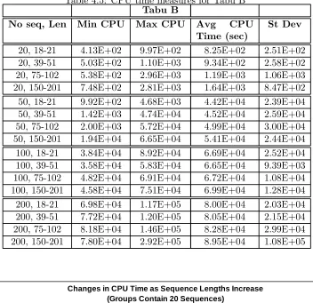
Table 4.5 displays the minimum, maximum, average and standard deviation of the CPU times for the 10 runs of Tabu B. The CPU time is affected by increases in the sequence length and number of sequences in an alignment. Additionally, the starting solution of a tabu search has an impact on the variability of the CPU time. If the tabu search randomly starts at a good solution, then it would take less time for the algorithm to stabilize as compared with a poor starting solution.

hours for both of these MSA programs. However, for both of these algorithms, the average CPU time for an MSA with 20 sequences that vary in length from 18-21 base pairs is only around 9-13 minutes.

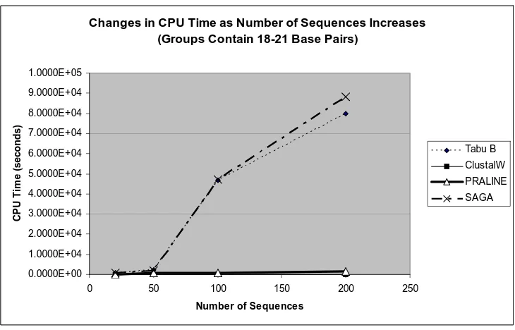
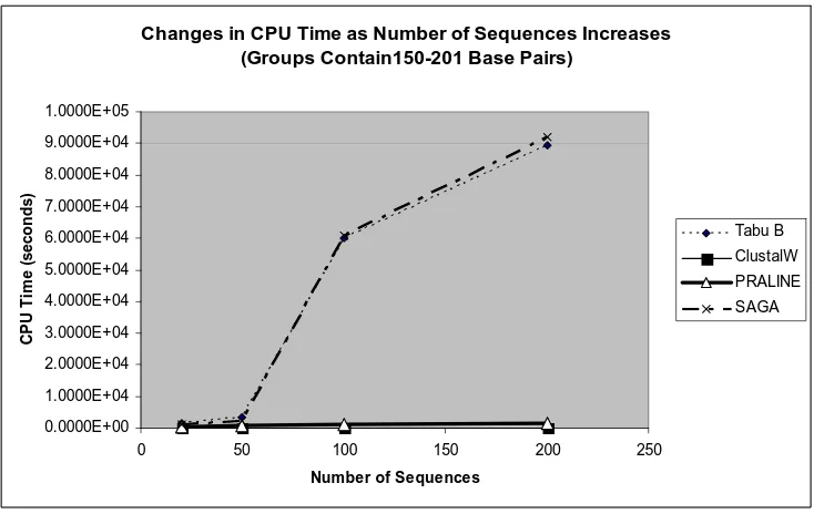
An increase in the sequence lengths, slightly increases the CPU time for each of the alignment programs. Figures 4-1 and 4-2 display the changes in the CPU time as the lengths of the sequences increase. For the group containing 20 sequences that vary in length from 18-21 base pairs, the Tabu B CPU time is 9.9 minutes. Where as, the Tabu B CPU time is 27.3 minutes for the group containing 20 sequences that vary in length from 150-201 base pairs. The CPU time for ClustalW and PRALINE are not significantly affected by changes in the number of sequences or the sequence lengths in an MSA. Each of the four algorithms would be efficient for aligning sequences with more than 200 base pairs. Because the CPU time for SAGA and Tabu B is extremely sensitive to an increase in the number of sequences in an MSA, these algorithms should ideally be used to align fewer that 200 sequences.

4.3.3

Tabu B with HMM Local Improvement Algorithm vs. SAGA

Table 4.4: Average CPU times from ClustalW, SAGA, PRALINE and Tabu B

No Seq, Len CPU Time

(sec)

No Seq, Len CPU Time

(sec)

Clus 20, 18-21 1.6560E+01 100, 18-21 2.1130E+01

SAG 20, 18-21 5.9469E+02 100, 18-21 6.7138E+04

PRA 20, 18-21 5.2282E+01 100, 18-21 9.1547E+02

TabB 20, 18-21 8.2471E+02 100, 18-21 6.6921E+04

Clus 20, 39-51 1.6760E+01 100, 39-51 2.1870E+01

SAG 20, 39-51 6.1379E+02 100, 39-51 6.6908E+04

PRA 20, 39-51 1.9252E+02 100, 39-51 9.4259E+03

TabB 20, 39-51 9.3405E+02 100, 39-51 6.6485E+04

Clus 20, 75-102 1.7480E+01 100, 75-102 2.2100E+01

SAG 20, 75-102 9.2731E+02 100, 75-102 6.9336E+04

PRA 20, 75-102 2.0379E+02 100, 75-102 1.0370E+03

TabB 20, 75-102 1.1917E+03 100, 75-102 6.7170E+04

Clus 20, 150-201 1.7710E+01 100, 150-201 2.4420E+01

SAG 20, 150-201 1.0796E+03 100, 150-201 7.1002E+04

PRA 20, 150-201 3.2482E+02 100, 150-201 1.1045E+03

TabB 20, 150-201 1.6351E+03 100, 150-201 6.9893E+04

Clus 50, 18-21 2.0200E+01 200, 18-21 2.2730E+01

SAG 50, 18-21 1.9524E+03 200, 18-21 8.8215E+04

PRA 50, 18-21 6.1844E+02 200, 18-21 1.3908E+03

TabB 50, 18-21 4.4159E+04 200, 18-21 7.9964E+04

Clus 50, 39-51 2.0230E+01 200, 39-51 2.3150E+01

SAG 50, 39-51 2.0148E+03 200, 39-51 8.3958E+04

PRA 50, 39-51 6.0957E+02 200, 39-51 1.4103E+03

TabB 50, 39-51 4.5236E+04 200, 39-51 8.0453E+04

Clus 50, 75-102 2.0340E+01 200, 75-102 2.5430E+01

SAG 50, 75-102 2.1775E+03 200, 75-102 9.0125E+04

PRA 50, 75-102 7.1381E+02 200, 75-102 1.4947E+03

TabB 50, 75-102 4.9929E+04 200, 75-102 8.2833E+04

Clus 50, 150-201 2.1160E+01 200, 150-201 6.7890E+01

SAG 50, 150-201 2.3025E+03 200, 150-201 9.1833E+04

PRA 50, 150-201 7.1665E+02 200, 150-201 1.6056E+03

Table 4.5: CPU time measures for Tabu B

Tabu B

No seq, Len Min CPU Max CPU Avg CPU

Time (sec)

St Dev

20, 18-21 4.13E+02 9.97E+02 8.25E+02 2.51E+02 20, 39-51 5.03E+02 1.10E+03 9.34E+02 2.58E+02 20, 75-102 5.38E+02 2.96E+03 1.19E+03 1.06E+03 20, 150-201 7.48E+02 2.81E+03 1.64E+03 8.47E+02 50, 18-21 9.92E+02 4.68E+03 4.42E+04 2.39E+04 50, 39-51 1.42E+03 4.74E+04 4.52E+04 2.59E+04 50, 75-102 2.00E+03 5.72E+04 4.99E+04 3.00E+04 50, 150-201 1.94E+04 6.65E+04 5.41E+04 2.44E+04 100, 18-21 3.84E+04 8.92E+04 6.69E+04 2.52E+04 100, 39-51 3.58E+04 5.83E+04 6.65E+04 9.39E+03 100, 75-102 4.82E+04 6.91E+04 6.72E+04 1.08E+04 100, 150-201 4.58E+04 7.51E+04 6.99E+04 1.28E+04 200, 18-21 6.98E+04 1.17E+05 8.00E+04 2.03E+04 200, 39-51 7.72E+04 1.20E+05 8.05E+04 2.15E+04 200, 75-102 8.18E+04 1.46E+05 8.28E+04 2.99E+04 200, 150-201 7.80E+04 2.92E+05 8.95E+04 1.08E+05

Changes in CPU Time as Sequence Lengths Increase (Groups Contain 20 Sequences)

0.0000E+00 2.0000E+02 4.0000E+02 6.0000E+02 8.0000E+02 1.0000E+03 1.2000E+03 1.4000E+03 1.6000E+03 1.8000E+03

0 50 100 150 200 250

Length of Longest Sequence in Group

C P U Ti m e ( s e c on ds ) Tabu B ClustalW PRALINE SAGA

Changes in CPU Time as Sequence Lengths Increase (Groups Contain 200 Sequences)

0.0000E+00 1.0000E+04 2.0000E+04 3.0000E+04 4.0000E+04 5.0000E+04 6.0000E+04 7.0000E+04 8.0000E+04 9.0000E+04 1.0000E+05

0 50 100 150 200 250

Length of Longest Sequence in Group

C P U Ti m e ( s e c on ds ) Tabu B Clustal W PRALINE SAGA

Figure 4-2: CPU time vs. Sequence length in MSAs with 200 sequences

Changes in CPU Time as Number of Sequences Increases (Groups Contain 18-21 Base Pairs)

0.0000E+00 1.0000E+04 2.0000E+04 3.0000E+04 4.0000E+04 5.0000E+04 6.0000E+04 7.0000E+04 8.0000E+04 9.0000E+04 1.0000E+05

0 50 100 150 200 250

Number of Sequences

C P U T im e ( s eco n d s) Tabu B ClustalW PRALINE SAGA

Changes in CPU Time as Number of Sequences Increases (Groups Contain150-201 Base Pairs)

0.0000E+00 1.0000E+04 2.0000E+04 3.0000E+04 4.0000E+04 5.0000E+04 6.0000E+04 7.0000E+04 8.0000E+04 9.0000E+04 1.0000E+05

0 50 100 150 200 250

Number of Sequences

C P U T im e ( s eco n d s) Tabu B ClustalW PRALINE SAGA

Figure 4-4: CPU time vs. Number of sequences in an MSA(with 150-201 BP) of an MSA containing fewer than 50 sequences.

Table 4.6: Improvement in MSA score for Tabu B with HMM

No Seq, Len % Improvement in SP Score

20, 18-21 0.986 20, 39-51 5.869 20, 75-102 2.483 20, 150-201 0.3665 50, 18-21 1.961 50, 39-51 0.6532 50, 75-102 7.659 50, 150-201 3.025

Table 4.7: MSA scores for the Tabu B with HMM and SAGA

No Seq, Len Tabu B + HMM SAGA Score