Data and Task Scheduling
in Distributed Computing Environments
Magdalena Szmajduch
Department of Computer Science, Cracow University of Technology, Cracow, Poland
Abstract—Data-aware scheduling in today’s large-scale het-erogeneous environments has become a major research and engineering issue. Data Grids (DGs), Data Clouds (DCs) and Data Centers are designed for supporting the process-ing and analysis of massive data, which can be generated by distributed users, devices and computing centers. Data scheduling must be considered jointly with the application scheduling process. It generates a wide family of global opti-mization problems with the new scheduling criteria including data transmission time, data access and processing times, re-liability of the data servers, security in the data processing and data access processes. In this paper, a new version of the Expected Time to Compute Matrix (ETC Matrix) model is defined for independent batch scheduling in physical net-work in DG and DC environments. In this model, the com-pletion times of the computing nodes are estimated based on the standard ETC Matrix and data transmission times. The proposed model has been empirically evaluated on the static grid scheduling benchmark by using the simple genetic-based schedulers. A simple comparison of the achieved results for two basic scheduling metrics, namely makespan and average flowtime, with the results generated in the case of ignoring the data scheduling phase show the significant impact of the data processing model on the schedule execution times.
Keywords—data cloud, data grid, data processing, data schedul-ing, ETC Matrix.
1. Introduction
In the recent decade, we witness an explosive growth in the volume, velocity, and variety of the data available on the Internet. Pethabythes of data were created on a daily basis. The data is generated by the highly distributed users and various types sources like the mobile devices, sensors, individual archives, social networks, Internet of Things de-vices, enterprise, cameras, software logs, etc. Such data explosions has led to one of the most challenging research issues of the current Information and Communication Tech-nology (ICT) era: how to effectively and optimally manage and schedule such large data for unlocking information? Scheduling problems in the distributed computing envi-ronments are mainly defined based on the task processing CPU-related criteria, namely makespan, flowtime, resource utilization, energy consumption and many others [1]. In such cases, all data-related criteria, like the data transmis-sion time, data access rights, data availability (replication) and security in data access issues are mostly ignored. Usu-ally it is assumed, that transmission is very fast, data ac-cess rights are granted, due to the single domain of LANs
and clusters (even if the whole infrastructure is highly dis-tributed), so there is no need for special data access man-agement. Obviously, the situation is very different in cur-rent large scale setting, where data sources needed for task completion can be located at different sites under different administrative domains.
Data-aware scheduling has been explored already in many research in cluster, grid and recently cloud comput-ing [2], [3]. Most of the current efforts are focused on the data processing optimization, storage (loads of the data servers) in the data centers or scheduling of data trans-mission and data location [4] for efficient resource/storage utilization or energy-effective scheduling in large-scale data centers [5], [6]. A recent example is that of GridBatch [7] for large scale data-intensive problems on cloud infrastruc-tures. However, the large amount of data to be efficiently processed remains a real research challenge, especially in the recent Big Data era. One of the key issues contributing to the massive processing efficiency is the scheduling with data transmission requirements.
In this paper, a new data-aware Expected Time to Compute Matrix (ETC Matrix) scheduling model is defined for com-putational grids and physical layers of the cloud systems, which takes into account new criteria such as data trans-mission and decoupling of data from processing [8]–[10]. The main aim of this work is to integrate the above cri-teria into a multi-objective optimization model in a sim-ilar way that it has been provided for computational grid scheduling with ETC Matrix [11]. However, the grid sched-ulers in presented model must take into account the features of both Computational Grid (CG) and Data Grid (DG) in order to achieve desired performance of grid-enabled ap-plications [12], [13]. Therefore, in this paper a general data-aware independent batch task scheduling problem is considered.
The remainder of the paper is structured as follows. The data-aware ECT Matix model for independent batch scheduling and main scheduling criteria are defined in Section 2. The empirical results are analyzed in Section 3. The paper is summarized in Section 4.
2. Data-aware Expected Time to
Compute (ETC) Matrix Model
Let’s consider a simple batch scheduling problem in com-putational physical infrastructure (big distributed cluster, grid or physical layer of the cloud system), where the tasksU1 U2 Un CC Cloud cluster Cloud cluster CC CC
Cluster cloud manager Cloud local scheduler
CH CH CH CH DH DH DH DH DH DH DH DH DH DH Data center
Data host Computational host
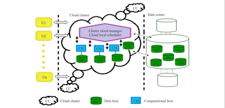
Fig. 1. Data-aware meta-task grid scheduling problem.
are processed independently and require multiple data sets from different heterogeneous data hosts. These data sets may be replicated at various locations and can be trans-ferred to the computational grid through the networks of various capabilities. A possible variant of this scenario is presented in Fig. 1.
The components of the whole system, task and data struc-tures in such scenario can be defined as follows:
– a batch of tasksN={t1, . . . ,tn}is defined as a meta-task structure,
– a set of computing grid nodes M ={m1, . . . ,mm} available for a given batch;
– a set of data-files F ={f1, . . . ,fr} needed for the batch execution,
– a set of data-hostsD={dh1, . . . ,dhs} dedicated for the data storage purposes, having the necessary data services capabilities.
The computational load of the meta-task is defined as atasks workload vectorW Lbatch= [wl1, . . . ,wln], wherewlj is the estimated computational load of tasktj(expressed in millions of instructions (MI). Each tasktjrequires for its ex-ecution the following set of data filesFj={f(1,j), . . . ,f(r,j)} (Fj⊆Fbatch), which is replicated and allocated at the fol-lowing data serversDHj.1
The computing capacity of computational servers available for a given batch is defined by acomputing capacity vector CCbatch= [cc1, . . . ,ccm], wherecci denotes the computing
1DH
jis a subset ofDH. Each filef(p,j)∈Fj(p∈ {1,... ,r}) is replicated on the servers fromDHj. It is assumed that each data host can serve multiple data files at a time and data replication is a priori defined as a separate replication process.
capacity of the server i expressed in million instructions per second (MIPS). The estimation of the prior load of each machine from Mbatch can be represented by a ready times vector ready times(batch)= [ready1, . . . ,readym]. An Expected Time to Compute (ETC) matrix model [11] is used for estimation of the completion times of tasks as-signed to a given computational server. Usually, the ele-ments of the ETC matrix can be computed as the ratio of the coordinates ofW LandCCvectors, namely:
ETC[i][j] =wlj
cci
. (1)
The values ofETC[j][i]for each pair machinemi and task tjin Eq. (1) depend mainly on the processing speeds of the machines, but need also express the heterogeneity of tasks and resources in the system. Therefore, in this approach the Gaussian distribution for generating the coordinates of both W L andCC vectors is used. Additionally, in data-aware scheduling, there is a need to estimate the data transfer time. For each data file fc j∈F (c∈ {1, . . . ,r}) necessary for the execution of the task tj, the time required to transfer this file from the data hostdhd∈Dto the servermi is denoted T Ti j[c][d]and can be calculated in the following way:
T Ti j[c][d] =RES[c][d] +
Size[fc j]
B[dhd,i], (2)
whereRES[c][d]is a response time of the data serverdhd and is defined as a difference between the request time to dhd and the time when the first byte of the data file fc is received at the computational server mi for computing the task tj (note, that the values of i and j are fixed here). The Size[fc,j] denotes the size (in Mbits) of the data file fc needed for execution of the tasktj, and byB[dhd,i]the
bandwidth of logical link (in Mbits/time unit) betweendhd andmi.
RES[c][d] are the elements of the Data Response Times MatrixRESs×r. In presented approach, the Gamma distri-bution [14] for generating those data response times is used. This method is widely used for estimation of the data trans-fer times [15]. It is similar to the Coefficient-of-Variation (CVB) [16] method used for generating the stochastic ma-trices with highly distributed two-dimensional random vari-ables. It may be used also for generation ETC matrices [1]. The key parameters for this method are defined as follows: – the cumulative estimated response times of all data servers while transferring an “average” data file, resave,
– the variance in the response times of data server, svardh,
– the variance in the heterogeneity of data files,rvarf. The parameters resave and svardh are used for estimating the response times RES[cˆ][d] of the data servers for the file fcˆwith the “average” data server speed in the systems. The times RES[cˆ][d] are generated by using the gamma distribution with the shape and scale parameters denoted byαs andβs respectively. That is:
RES[cˆ][d] =Gamma(αs,βs), (3) where: αs= 1 svardh2 , (4) βs= resave αs . (5)
The generated vector of RES[cˆ][d] parameters (dhd∈D) defines one row (indexed bycˆ) of the RES matrix. Each element of this row is then used for generating one column of the RES matrix, that is:
RES[c][d] =Gamma(αr,βr), (6) where: αr= 1 rvar2 f , (7) βr= RES[cˆ][d] αr . (8) and fc∈F,c6=cˆ.
The resources completion times are the main scheduling parameters in the ETC matrix model. It is denoted by
completion[j][i] estimated completion time for the task tj
on machinemi. It is defined as the wall-clock time taken for the task from its submission till completion. In data-aware scheduling, it depends on computing and transmis-sion times specified in Eqs. (1) and (2). The impact of the data transfer time on the task completion time depends on
Tf(k,j) Tf(k,j) Tf(2 ),j T f(2 ),j Tf(1 ),j T f(1 ),j Tf(3 ),j ETC[i][j] ETC[i][j] (a) (b) Time Time
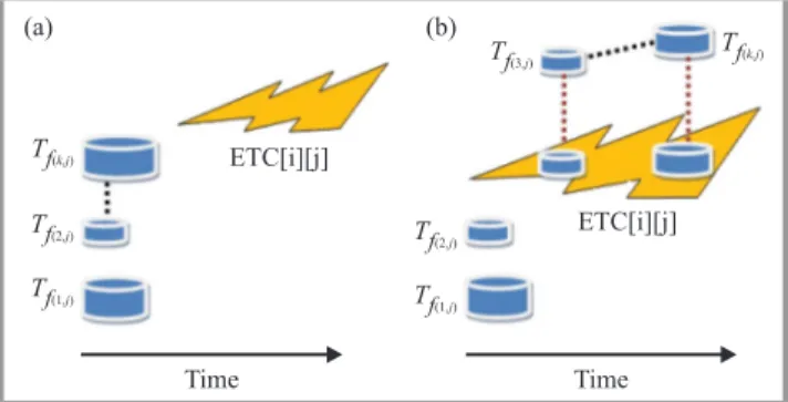
Fig. 2. Two variants of task completion times estimation assigned to the machinemiwithkdata files needed for the task execution.
the mode, in which the data files are processed by the task. Figure 2 presents two such scenarios (see also [17]). In the “a” scenario, data files needed for the execution of task tj are transferred to the computational server before the calculation of all tasks assigned to this server, includ-ing task tj. The number of simultaneous data transfers determines the bandwidth available for each transfer. The completion time of the tasktj on machine mi in this case is defined as follows:
completiona[i][j] = max
fc j∈F;dhd∈D
T Ti j[[c][d] +ETC[i][j]. (9)
In the “b” scenario, some of the data files are transferred as in scenario “a”, but the major data needed for the execu-tion of each task assigned to the servermi (also tasktj) is transferred during the execution of the tasks. In this case, the transfer times of the streamed data files are masked by the computation times of the tasks. The completion time of the task tj on machinemi in this scenario is defined in the following way:
completionb[i][j] = max fc j∈Fbj T Ti j[c][d] +
∑
fl j∈[F\Fbj] (T Ti j[l][d] +ETC[i][j]) (10)where Fbj denotes a set of data files which are transferred prior the execution of the task tj and in fact all tasks as-signed to this server.
In this paper the data hosts as the data storage centers are considered, which are separated from the computing re-sources.
2.1. Scheduling Criteria
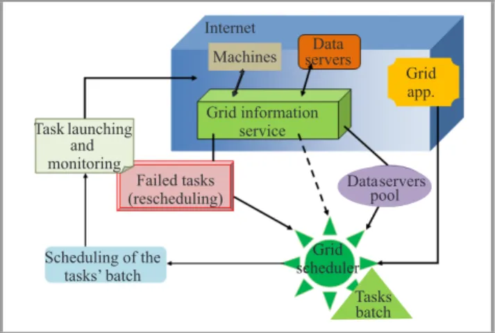
A general data-aware batch scheduling process is realized in the following steps:
• get the information on available resources, • get the information on pending tasks,
• get the information on data hosts where data files for tasks completion are required,
• prepare a batch of tasks and compute a schedule for that batch on available machines and data hosts, • allocate tasks,
• monitor (failed tasks are re-scheduled).
These steps can be graphically represented as in Fig. 3.
Grid app. Grid scheduler Scheduling of the tasks’ batch Failed tasks (rescheduling) Task launching and monitoring Grid information service Data servers Tasks batch Dataservers pool Machines Internet
Fig. 3. Phases of the data-aware batch scheduler.
The main objectives in data-aware scheduling are similar to the objectives formulated for conventional scheduling in distributed computational systems without data files [1] and include minimization of completion time, makespan and average flowtime, namely:
• Minimizing completion time of the task batch defined in the following way:
completionbatch=
∑
tj∈Nbatch;mi∈Mbatch
completion[i][j], (11)
wherecompletion[i][j]is defined as in Eq. 9 or Eq. 10 depending on considered data transfer scenario; • Minimizing makespanCmax:
Cmax= max
mi∈Mbatch
completion[i], (12)
wherecompletion[i]is computed as the sum of com-pletion times of tasks assigned to machinemi calcu-lated by using Eq. 9 or Eq. 10;
• Minimizing average flowtimeF˜. A flowtime for a ma-chinemican be calculated as a workflow of the tasks sequence on a given machinemi, that is to say:
F[i] =completion[i]. (13)
The cumulative flowtime in the whole system is de-fined as the sum ofF[i]parameters, that is:
F=
∑
i∈M
F[i]. (14)
Finally, the scheduling objective is to minimize the average flowtime F˜ for one machine defined as fol-lows:
˜
F=F
m. (15)
In the above equations the ETC matrix model is used which is very useful for the formal definition of all main scheduling criteria. Thecompletion[i]parameters are the coordinates of the completion vector completion=
[completion[1], . . .,completion[m]]T. The extended list of
the scheduling criteria defined in terms of completion times and by using the ETC matrix model can be found in [1].
3. Experiments
The main aim of the experiments is to illustrate the impact of the data transfer times on the completion times of the physical resources in the system. The values of makespan and average flowtime calculated by using Eqs. 12 and 15 are compared with the case of conventional scheduling, where data transfer times are ignored. In such a case it is assumed that all necessary data is stored at computa-tional nodes and ready for use, which is unrealistic. For the analysis both data transfer scenarios specified in Sec-tion 2, namely scenario “a” and scenario “b” are considered. Therefore, the completion times in Eq. 12 are estimated by using Eq. 9 in the first scenario, and Eq. 10 in the second scenario.
The experiments were provided with simple genetic-based scheduler defined in Subsection 3.2, which has been used already as grid batch scheduler by many researchers in the domain (see [18], [19] and [20]). There are many other genetic grid and cloud schedulers that are more effective in the optimization of the makespan and flowtime crite-ria [1]. However, such effectiveness is not the main aim of this analysis. All those schedulers are also quite complex methods from the implementation and scaling perspectives. Therefore, a simple scheduler was used to show, how much the data transfer may delay the execution of schedules.
3.1. Data Grid Simulator
For the experiments the Sim-G-Batch simulator defined in [1] is used. The basic set of the input data for the simulator includes:
– the workload vector of tasks,
– the computing capacity vector of machines, – the vector of prior loads of machines, and
– the ETC matrix of estimated execution times of tasks on machines.
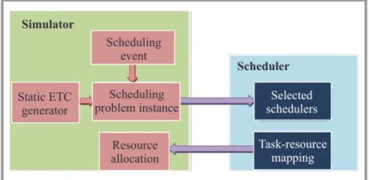
The Sim-G-Batch simulator is highly parametrized to re-flect the various realistic scheduling scenarios. In this
paper, the author limited the experiments to the static batch scheduling benchmarks. Fig. 4 presents the selected modules of Sim-G-Batch, which are active in performed experiments. Simulator Scheduler Static ETC generator Scheduling event Scheduling problem instance Resource allocation Selected schedulers Task-resource mapping
Fig. 4. Selected components of Sim-G-Batch simulator for the experiments on static benchmarks.
The benchmark for small static grid was generated by the Static ETC Generator module of the simulator. The in-stances in this benchmark are classified into 12 types of ETC matrix, according to task heterogeneity, machine het-erogeneity and consistency of computing. These instances are labeled by the following parameters [1]:
Gauss xx yyzz.0 (16)
where:
– Gaussis the Gaussian distributions used in
generat-ing theW LandCCvectors,
– xx denotes the type of consistency of ETC matrix (cˆ – consistent, i˜ˆ– inconsistent, and sˆ– semi-con-sistent),
– yyindicates the heterogeneity of tasks (hi– high het-erogeneity, andlo– low heterogeneity),
– zzexpresses the heterogeneity of the resources (hi– high, andlo– low).
The ETC matrix is consistent if for each pair of the re-sourcesmi and mˆi the following condition is satisfied: if the completion time of some tasktj is shorter at resource mi than at resourcemiˆ, then all tasks can be executed (and finalized) faster atmi than atmˆi. The inconsistency of the matrixETCmeans that there no consistency relation among resources. Semi-consistentETC matrices are inconsistent matrices having a consistent sub-matrix.
The following probability distributions have been used in the experiments: N(1000; 175) for resources and
N(250000000; 43750000)for tasks, whereN(α,σ)denotes
the Gaussian distribution with meanα and standard devi-ation σ. The computing cluster network is composed of 64 nodes (machines) and there are 1024 tasks submitted for scheduling. In addition, 32 data servers and 2048 data files for a given batch is assumed. The data hosts response times are generated by using the Gamma distribution
ac-cording to the description in Section 2 with the following parameters resave=10, and 0.1≤svardh , rvarf ≤0.35. The sizes of data files and the bandwidth are generated by the uniform distributions defined for the following intervals
[2; 1600]and[10; 100]respectively.
3.2. Genetic-based Scheduler
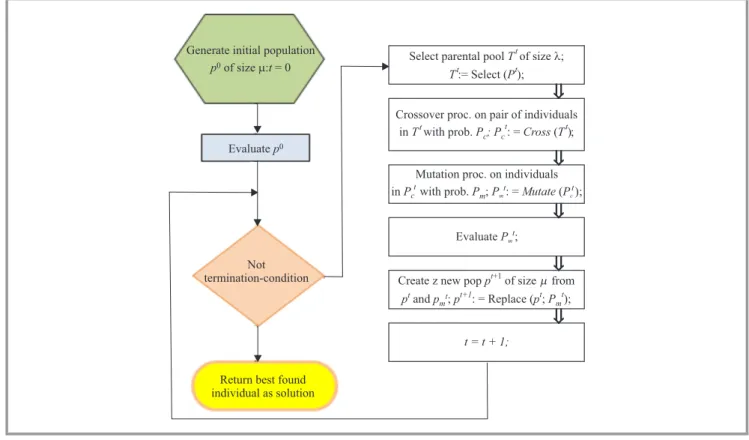
Genetic-based meta-heuristics have shown great potential to solve multi-criteria grid or cloud scheduling problems by trading-off various preferences and goals of the system users and managers [21], [22]. Simple single-population genetic schedulers can be promoted as the effective meth-ods for solving small-scale static scheduling problems. In the experiments a simple (µ+λ)-like evolutionary sched-uler is used similar to those used for solving classical com-binatorial optimization problems [23]. The general schema of this scheduler is presented in Fig. 5.
In the implementation of the scheduler two schedules’ representations are used, namely direct representation and permutation-based encoding. In the direct represen-tation, each schedule is defined as the schedule vector x= [x1, . . . ,xn]T, where xi∈ {1, . . . ,m} are the labels of the computational resources, to which the particular tasks labeled by1, . . . ,nare assigned. In permutation-based rep-resentation, for each resource a sequence of tasks assigned to that resource is defined. The tasks in the sequence are increasingly sorted with respect to their completion times. In this representation, some additional information about the numbers of tasks assigned to each machine is required. In this work the direct representation for the encoding of the individuals in the base populations denoted by Pt and Pt+1in Fig. 5 is used. The permutation-based representa-tion is necessary for the implementarepresenta-tion of the specialized genetic operators. Based on the results of tuning process provided in [18], [20] and [21], the optimal configuration of genetic operators for considered scheduler is defined as follows:
– selection – Linear Ranking, – crossover – Cycle Crossover, – mutation – Rebalancing, – replacement – Steady State.
All those genetic operators are commonly used in solving the large-scale combinatorial problems [23]. The main idea of the Cycle Crossover (CX) is identification of the cycle of alleles (positions). The existing cycles (of tasks) are kept unchanged. The remaining fragments in the parental strings are exchanged, and the resulting permutation strings are repaired if some task labels are duplicated. In rebal-ancing mutation, first the most overloaded machine mi is selected. Then two taskstj andtjˆare identified as follows: tˆj is assigned to another machinemˆi ,tj is assigned tomi andETC[iˆ][jˆ]≤ETC[i][j]. Then the assignments for tasks tj and tjˆ are interchanged. In Steady State replacement
Generate initial population of size : = 0 p0 mt Evaluatep0 Not termination-condition
Return best found individual as solution
Select parental poolTtof size ;l
:= Select ( ); Tt Pt
Crossover proc. on pair of individuals inTtwith prob.P ; Pc ct: =Cross T( );t
Mutation proc. on individuals inPcwith prob.Pm;P : =Mutate P( );
t t t
m c
EvaluatePm;
t
Create z new poppt+1of size from and ; : = Replace ( ; ); pt p t pt+1 p Pt t
m m
t = t + 1;
Fig. 5. General template of the GA-scheduler implementation.
method, the set of the highest quality offsprings replaces the similar set (of the same cardinality) of the solutions of the worst quality in the old base population.
Table 1
Key parameters of the GA-scheduler (n– the number of tasks in the batch)
Parameter Value µ 4·(log2n−1) λ µ/3 mut prob 0.15 cross prob 0.9 nb of epochs 20·n
max time to spend 25s
The values of the control parameters for the genetic sched-uler are presented in Table 1. The number of individuals in base populations shown asPt andPt+1in Fig. 5 is denoted byµ,λ is the number of individuals in offspring popula-tionsTt,Pt
candPmt. The parameterscross prob,mut prob are used for the notation of of the crossover and muta-tion probabilities. Thenb o f epochs denotes the maximal number of main loop executions of the algorithm. Each loop execution is interpreted as genetic epoch. The maxi-mal number of such epochs is defined as the main global stopping criterion for the scheduler. However, if the execu-tion of those epochs will take much time, the algorithm is stopped after 25 s (max time to spend).
3.2.1. Results
Tables 2 and 3 present the average values of makespan and average flowtime achieved in the scenarios “a” and “b” (see Section 2) and No data transfer case. Each experiment has been executed 30 times under the same configuration of all input parameters and data for simulator and sched-uler. Both tables present the results averaged over 30 in-dependent runs of the simulator with [±s.d.]s.d-standard deviation values.
Both makespan and average flowtime are expressed in ar-bitrary (but not concrete) time units.
In makespan optimization, scenario “b” is the case, where most of the achieved results are better than for the prior load of all data files before the task execution (scenario “a”). In the case of average flowtime optimization, the impact of the consistency of ETC matrix on the mode of the data transfer is even better illustrated. In all cases for consistent and semi-consistent matrices and for inconsistent matrices with high heterogeneity of computing resources, it is better to request just necessary data files during the computation (scenario “b”). The differences in the flowtime values in scenario “a” and scenario “b” are more significant than in the makespan case. However, in both makespan and flow-time optimizations, it is observed that the flowflow-time values are much higher in the case of additional data transfer times, than in the “data transfer-free” scheduling. In the case of inconsistent and semi-consistent ETC matrices, it is almost doubled.
Table 2
Makespan values in three scheduling scenarios
Instance Scenario “a” Scenario “b” No data transfer
Gauss c hihi 10020355.256 9621178.557 7506387.215 [±801234.852] [±998911.259] [±631202.153] Gauss c hilo 226250.310 213490.536 139974.423 [±19936.993] [±19343.184] [±10846.362] Gauss c lohi 459987.880 468466.775 238839.338 [±19323.273] [±22765.627] [±18892.634] Gauss c lolo 6761.231 6926.864 5109.783 [±770.132] [±240.019] [±258.635] Gauss i hihi 6093651.564 5866694.694 3069945.734 [±702187.019] [±1191799.837] [±877534.287] Gauss i hilo 146705.432 145813.231 75588.928 [±4451.987] [±4062.978] [±3184.872] Gauss i lohi 198611.123 187170.435 109343.652 [±20873.994] [±19351.412] [±25636.425] Gauss i lolo 5194.763 5117.546 2616.643 [±122.543] [±138.321] [±156.792] Gauss s hihi 8085209.000 7961402.628 4254421.785 [±578839.375] [±663325.239] [±853673.523] Gauss s hilo 186281.400 167445.544 99009.537 [±14746.582] [±10831.231] [±8763.471] Gauss s lohi 215692.530 220844.573 126822.639 [±64353.500] [±53473.637] [±98723.537] Gauss s lolo 6856.982 6554.654 3498.623 [±453.321] [±643.308] [±764.364]
4. Conclusions and Research
Directions
In this paper the new version of ETC Matrix model for batch scheduling in the physical clusters was defined, where separate computing and data servers are located. In this model, the completion times of all tasks assigned to the computing nodes of the network have included the data transmission times. Two data transmission scenarios were considered with prior load of all files necessary for the ex-ecution of assigned tasks, and with the ad-hoc delivery of just requested (necessary) data files during the task execu-tion. The results of the performed experiments show that omitting the data transfer phase in the scheduling process may lead to the bad estimations of the scheduling times, and more general scheduling costs.
The performed analysis in its early stage. The author plans to extend it to the virtual resources and databases and the extended cloud infrastructures, where the mobile devices (smartphones, tablets, laptops, etc.) are considered as the computational nodes of the physical cloud layer and can additionally store and generate the data. This will allow to validate proposed model in much more realistic cloud scheduling scenarios, but also will increase the complexity of the scheduling problem.
References
[1] J. Kołodziej,Evolutionary Hierarchical Multi-Criteria
Metaheuris-tics for Scheduling in Large-Scale Grid Systems. Studies in
Com-putational Intelligence Serie, vol. 419. Berlin-Heidelberg: Springer,
2012.
[2] H. Casanova, G. Obertelli, F. Berman, and R. Wolski, “The AppLeS parameter sweep template: user-level middleware for the grid”, in
Proc. 2000 ACM/IEEE Conf. on Supercomputing SC 2000), Dallas,
TX, USA, 2000.
[3] R. Buyya, M. Murshed, D. Abramson, and S. Venugopal, “Schedul-ing parameter sweep applications on global Grids: a deadline and budget constrained cost-time optimization algorithm”,Softw. Pract.
Exper., vol. 35, no. 5, pp. 491–512, 2005.
[4] T. Kosar and M. Balman, “A new paradigm: Data-aware schedul-ing in grid computschedul-ing”,Future Gener. Comp. Syst., vol. 25, no. 4, pp. 406–413, 2009.
[5] J. Kołodziej, S. U. Khan, and F. Xhafa, “Genetic algorithms for energy-aware scheduling in computational grids”, inProc. 6th IEEE
Int. Conf. P2P, Parallel, Grid, Cloud, and Internet Comput. 3PGCIC,
Barcelona, Spain, 2011, pp. 17–24.
[6] G. L. Valentiniet al., “An overview of energy efficiency techniques in cluster computing systems”, Cluster Comput., vol. 16, no. 1, pp. 3–15, 2011.
[7] H. Liu and D. Orban, “GridBatch: Cloud Computing for Large-Scale Data-Intensive Batch Applications”, in Proc. 8th IEEE Int.
Symp. Cluster Comput. and the Grid CCGRID 2008, Lyon, France,
2008, pp. 295–305.
[8] J. Kołodziej and F. Xhafa, “A game-theoretic and hybrid genetic meta-heuristic model for security-assured scheduling of independent jobs in computational grids”, inProc. Int. Conf. Complex, Intell.
Table 3
Flowtime values in three scheduling scenarios
Instance Scenario “a” Scenario “b” No data transfer
Gauss c hihi 1865377511.523 1739118543.763 1039888902.5391 [±62551800.572] [±108789000.698] [±87276600.974] Gauss c hilo 38856381.645 37530920.723 26758471.974 [±1855790.927] [±1572700.673] [±1761150.029] Gauss c lohi 45736995.532 44536681.673 33480185.582 [±1662420.635] [±4060500.216] [±4362160.982] Gauss c lolo 130462.627 1233817.453 891295.864 [±51414.523] [±56050.981] [±34862.735] Gauss i hihi 629477886.653 578364926.537 349268315.516 [±121534968.473] [±2075608399.845] [±147994960.873] Gauss i hilo 23654208.787 23615230.173 12427872.618 [±894854.731] [±749330.642] [±680981.333] Gauss i lohi 23344908.394 23417596.793 12718274.271 [±2909746.766] [±3324080.433] [±4395729.934] Gauss i lolo 826185.831 829731.985 450123.843 [±25385.445] [±34978.732] [±32745.674] Gauss s hihi 1048266515.861 994973664.431 522894137.524 [±103674264.922] [±90143000.322] [±107532000.119] Gauss s hilo 29959243.952 28415261.227 16871684.228 [±1173072.427] [±1556320.435] [±2152640.536] Gauss s lohi 22655131.553 21648611.228 14923174.777 [±4981350.195] [±6657510.587] [±7907100.555] Gauss s lolo 1005375.388 998332.695 582565.111 [±66981.229] [±67459.762] [±44452.203]
[9] L. Wang and S. U. Khan, “Review of performance metrics for green data centers: a taxonomy study”, J. Supercomput., vol. 63, no. 3, pp. 639–656, 2013.
[10] S. Zeadally, S. U. Khan, and N. Chilamkurti, “Energy-efficient net-working: past, present, and future”, J. Supercomput., vol. 62, no. 3, pp. 1093–1118, 2012.
[11] S. Ali, H. J. Siegel, M. Maheswaran, and D. Hensgen, “Task execu-tion time modeling for heterogeneous computing systems”, inProc.
9th Heterogen. Comput. Worksh. HCW 2000, Cancun, Mexico, 2000,
pp. 185–199.
[12] J. Kołodziej and F. Xhafa, “Meeting security and user behaviour requirements in grid scheduling”, Simul. Model. Pract. Theory, vol. 19, no. 1, pp. 213–226, 2011.
[13] J. Kołodziej and F. Xhafa, “Integration of task abortion and security requirements in GA-based meta-heuristics for independent batch grid scheduling”, Comp. Mathem. Appl., vol. 63, no. 2, pp. 350–364, 2011.
[14] L. L. Lapin, Probability and Statistics for Modern Engineering, 2nd ed. Long Grove, USA: Waveland Pr. Inc., 1998.
[15] A. Deshpande, Z. G. Ives, and V. Raman, “Adaptive query process-ing”,Foundation and Trends in Databases, vol. 1, no. 1, pp. 1–140, 2007.
[16] S. Ali, H. J. Siegel, M. Maheswaran, and D. Hensgen, “Represent-ing task and machine heterogeneities for heterogeneous comput“Represent-ing systems”,Tamkang J. Sci. Engin., vol. 3, no. 3, pp. 195–207, 2000. [17] S. Venugopal and R. Buyya, “An SCP-based heuristic approach for scheduling distributed data-intensive applications on global grids”,
J. Parallel Distrib. Comp., vol. 68, pp. 471–487, 2008.
[18] F. Xhafa, L. Barolli, and A. Durresi, “Batch mode schedulers for grid systems”,Int. J. Web and Grid Serv., vol. 3, no. 1, pp. 19–37, 2007.
[19] F. Pinel, J. E. Pecero, P. Bouvry, and S. U. Khan, “A two-phase heuristic for the scheduling of independent tasks on computational grids”, inProc. of ACM/IEEE/IFIP Int. Conf. High Perform. Comput.
Simul. HPCS 2011, Istanbul, Turkey, 2011, pp. 471–477.
[20] J. Kołodziej and F. Xhafa, “Enhancing the genetic-based schedul-ing in computational grids by a structured hierarchical population”,
Future Gener. Comp. Syst., vol. 27, pp. 1035–1046, 2011.
[21] F. Xhafa and A. Abraham, “Computational models and heuristic methods for grid scheduling problems”,Future Gener. Comp. Syst., vol. 26, pp. 608–621, 2010.
[22] J. Kołodziej and S. U. Khan, “Multi-level hierarchic genetic-based scheduling of independent jobs in dynamic heterogeneous grid en-vironment”,Inform. Sci., vol. 214, pp. 1–19, 2012.
[23] Z. Michalewicz,Genetic Algorithms + Data Structures = Evolution
Programs. Berlin: Springer, 1992.
Magdalena Szmajduch is a
Ph.D. student of computer sci-ence in the Interdisciplinary Ph.D. Programme managed jointly by the Jagiellonian University in Cracow, Polish Academy of Science in Warsaw and Cracow University of Tech-nology. She is also the assistant professor at the Department of Computer Science of Cracow University of Technology. The main topic of her interest is data processing in large scale distributed dynamic systems. E-mail: [email protected]
Department of Computer Science Cracow University of Technology Warszawska st 24