ADN_Modelica: An Open Source Sequence-Phase Coupled Frame Program for Active Distribution Network Steady State Analysis

(1)

Article

ADN_Modelica: An Open Source Sequence-Phase

Coupled Frame Program for Active Distribution

Network Steady State Analysis

Yuntao Ju 1,_{*, Fuchao Ge}1_{, Yi Lin}2_{and Jing Wang}3

1_{College of Information and Electrical Engineering, China Agricultural University, Beijing 100083, China;} [email protected]

2 _{Electric Power Research Institute of Fujian Electric Power Limited Company, Fuzhou 350007, China;} [email protected]

3 _{China Electric Power Research Institute, Beijing 100192, China; [email protected]} * Correspondence: [email protected]; Tel.: +86-189-1124-1286

Abstract: Open source software such as OpenDSS has given a lot of help to distribution network researchers and educators. With high penetration of distributed renewable energy resources into distribution network, tradition distribution steady state analysis software such as OpenDSS is faced with difficulty in handling distributed generators. Three-phase distributed generators are often modeled in sequence frame while unbalanced distribution network are usually modeled in phase frame. So a load flow in sequence-phase coupled frame is proposed to handle models described in both frames. Voltage controlled DGs which are difficult to cope with in OpenDSS are handled in proposed program. The steady state analysis platform is programmed with open source Modelica language and the main aim of this paper is to introduce an open source platform for active distribution network steady analysis include load flow and short circuit analysis which can be easily adopted and improved by other educators and researchers.

Keywords: steady state analysis; Modelica; active distribution network

1. Introduction

Open source software has given a lot of help to power system researchers. As commercial software is closed source, algorithms of which are not easily to be improved for research. From the point of education, commercial software does not show clear flowchart of power system analysis such as load flow, transient simulation etc.

Power System Analysis Toolbox [1] presented by Federico Milano has provides a huge support to students and researchers of electrical engineering. This software is mainly used for transmission network while unbalanced distribution network analysis is not supported.

Matpower [2] proposed by Ray Daniel Zimmerman provides quick algorithm of load flow with the help of fast matrix and vector computation ability of Matlab.

OpenDSS [3] presented by Roger C. Dugan helps a lot on unbalanced distribution network analysis. As fixed point iteration method is deployed in OpenDSS, constant power distributed generators can be well coped with while voltage controlled distributed generators (DGs) may encounter severe convergence problem [4]. Load flow algorithm of Gridlab-D[5] encounters the similar problem. So fixed point iteration is not a suitable method to handle voltage controlled DGs, a newton approach proposed is presented in [6] to cope with this. Other open source work [7] has given a introduction on using Modelica language to analyze AC circuits while it can not cope with unbalanced distribution system.

(2)

can handle sequence-phase frame models simultaneously compared with other commercial distribution analysis software.

Open source software gives a lot of help to power system analysis. The main aim of this paper is to provide an open source platform which can be easily modified by other researchers.

2. Three-phase Modeling of Distribution Network

There are mainly two kinds of constraints to describe electric network. KCL and KVL belong to topology constraints and other constraints such as ohm’s constraints, PQ constraints belong to branch constraints. Firstly, KVL and KCL can be written as

b,re = n,re,

U AU (1)

b,im = n,im,

U AU (2)

b,re

0 ₌_{A I}T ,₍₃₎

b,im

0 ₌_{A I}T ,₍₄₎

where subscript b denotes branch quantities, subscript n denotes node quantities, subscript re

and subscript im denote real and imagine quantities, matrix A represents node-branch incidence

matrix. U and I represent voltage and current vector respectively.

Modelica is an equation-based simulator [10]. KCL and KVL constraints are naturally supported by Modelica, with definition of connector and flow. Node voltage quantities in network analysis is defined as connector while current is defined as flow variables.

Other branch constraints are generally expressed as

(

b,re, b,im, b,re, b,im

)

0

f U U I I = (5)

which represents relationship between branch voltage and branch current. The detail of various

branch constraints in steady state analysis are described as followings.

2.1. One-phase Impedance Branch

Single phase branch is frequently existed in low voltage distribution network. Denoting resistance and reactance of branch as R and X respectively, the branch voltage and branch current relationship can be written as

b,re b,re b,im,

U =RI -XI (6)

b,im b,im b,re.

U =RI +XI (7)

The branch constraints’ equations are described with Modelica language as follows.

model OnePhaseImpedance

extends Interfaces.OnePhaseBranch; parameter SI.Resistance R = 1; parameter SI.Reactance X=1; equation

vRe = R * iRe - X*iIm; vIm = R * iIm +X*iRe; end OnePhaseImpedance;

It can be seen from above that Modelica is equation-based simulator. So the branch constraints in the following section will be all described with equations clearly.

2.2. Two-phase Impedance Branch

Two-phase impedance branch can be seen as two branches with coupled impedance. The impedance matrix of branch 1 and branch 2 is given by

11 12

21 22 , two pha

R R

-é ù

ê ú

= ê_ê ú_ú

ë û

(3)

11 12

21 22 , two pha

X X

-é ù

ê ú

= ê_ê ú_ú

ë û

X (9)

where subscript 1 and 2 denote branch 1 and 2 respectively.

The coupled branch voltage and current relationship can be written as

,1 ,1

,2 ,2

j ,

b b

two pha two pha

b b

U I

U - - I

é ù é ù

ê ú₌ é ₊ ùê ú

ê ú ë ûê ú

ê ú ê ú

ë û ë û

R X

 

  (10)

where symbols with dot above represent complex quantities.

The complex variable form of (10) can be unfolded to four equations as follows.

b,1,re 11 b,1,re 12 b,2,re 11 b,1,im 12 b,2,im,

U =R I +R I -X I -X I (11)

U =R I +R I -X I -X I (12)

b,1,im 11 b,1,re 12 b,2,re 11 b,1,im 12 b,2,im,

U =X I +X I +R I +R I (13)

b,2,i 21 b,1,re 22 b,2,re 21 b,1,im 22 b,2,im.

U =X I +X I +R I +R I (14)

2.3. Three-phase Impedance Branch

Three-phase impedance branch can be seen as three branches with coupled impedance. The impedance matrix is given by

11 12 13

21 22 23

31 32 33

, three pha

R R R

-é ù

ê ú

= ê ú

ê ú

ë û

R (15)

11 12 13

21 22 23

31 32 33

, three pha

X X X

-é ù

ê ú

= ê ú

ê ú

ë û

X (16)

where subscript 1, 2, 3 denote branch 1, 2 ,3 respectively.

The three phase impedance branch constraints can be unfolded to six equations.

b,1,re 11 b,1,re 12 b,2,re 13 b,3,re 11 b,1,im 12 b,2,im 13 b,3,im,

U =R I +R I +R I -X I -X I -X I (17)

U =R I +R I +R I -X I -X I -X I (18)

U =R I +R I +R I -X I -X I -X I (19)

b,1,im 11 b,1,re 12 b,2,re 13 b,3,re 11 b,1,im 12 b,2,im 13 b,3,im,

U =X I +X I +X I +R I +R I +R I (20)

U =X I +X I +X I +R I +R I +R I (21)

b,3,im 31 b,1,re 32 b,2,re 33 b,3,re 31 b,1,im 32 b,2,im 33 b,3,im.

U =X I +X I +X I +R I +R I +R I (22)

2.4. One-phase Admittance Branch

Shunt admittance of distribution line, capacitors are model as admittance branch. The branch voltage and branch current relationship can be written as

b,re b,re b,im,

I =GU -BU (23)

b,im b,im b,re,

I =GU +BU (24)

where G represents conductance and B represents susceptance. For capacitor branch, G =0.

2.5. Two-phase Admittance Branch

(4)

11 12

21 22 , two pha

G G

-é ù

ê ú

= ê_ê ú_ú

ë û

G (25)

11 12

21 22 , two pha

B B

-é ù

ê ú

= ê ú

ê ú

ë û

B (26)

where subscript 1 and 2 denote branch 1 and 2 respectively.

The coupled branch voltage and current relationship can be written as

,1 ,1

,2 ,2

j ,

b b

two pha two pha

b b

I U

I - - U

é ù é ù

ê ú₌ é ₊ ùê ú

ê ú ë ûê ú

ê ú ê ú

ë û ë û

G B

 

  (27)

where symbols with dot above represent complex quantities.

The complex variable form of (27) can be unfolded to four equations as follows.

I =G U +G U -B U -B U (28)

I =G U +G U -B U -B U (29)

b,1,im 11 b,1,re 12 b,2,re 11 b,1,im 12 b,2,im,

I =B U +B U +G U +G U (30)

b,2,im 21 b,1,re 22 b,2,re 21 b,1,im 22 b,2,im.

I =B U +B U +G U +G U (31)

2.6. Three-phase Admittance Branch

Three-phase admittance branch can be seen as three branches with coupled admittance. The admittance matrix is given by

11 12 13

21 22 23

31 32 33

, three pha

G G G

-é ù

ê ú

= ê ú

ê ú

ë û

G (32)

11 12 13

21 22 23

31 32 33

, three pha

B B B

-é ù

ê ú

= ê ú

ê ú

ë û

B (33)

where subscript 1, 2, 3 denote branch 1, 2 ,3 respectively.

The three phase admittance branch constraints can be unfolded to six equations.

I =G U +G U +G U -B U -B U -B U (34)

I =G U +G U +G U -B U -B U -B U (35)

I =G U +G U +G U -B U -B U -B U (36)

I =B U +B U +B U +G U +G U +G U (37)

I =B U +B U +B U +G U +G U +G U (38)

b,3,im 31 b,1,re 32 b,2,re 33 b,3,re 31 b,1,im 32 b,2,im 33 b,3,im.

I =B U +B U +B U +G U +G U +G U (39)

2.6. Transformer

Distribution transformer is composed of one-phase ideal transformer and one-phase impedance. Firstly, we give the model of one- phase ideal transformer.

2.6.1. One-phase Ideal Transformer

(5)

Figure 1. One-phase Ideal Transformer

The coupled branch constraints can be written as

b,1 b,2,

U =kU (40)

b,1 b,2,

kI = -I (41)

where k denotes transformer ratio. Subscript 1 and 2 denotes branch 1 and 2 respectively. The equations can be written in real field

b,1,re b,2,re,

U =kU (42)

b,1,im b,2,im,

U =kU (43)

b,1,re b,2,re,

kI = -I (44)

b,1,im b,2,im.

kI = -I (45)

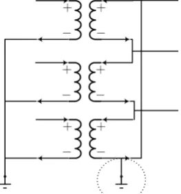
2.6.2. Three-phase Transformer

There are various connection type for three-phase transformer such as GrY/GrY, GrY/D, D/GrY etc. All of them can be formed with one-phase impedance branch and ideal transformer branch which are depicted in Figure 2.

(a) (b)

Figure 2. Two typical two-winding transformer connection: (a) GrY/GrY; (b) GrY/D

2.6.3. Network Anti-Floating Method

The network at secondary side of GrY/D transformer in the Figure 2(b) is floating which will result in convergence problem for load flow analysis. With adding anti-floating voltage reference such as ground to floating network as depicted in Figure 3, this convergence problem is handled. The node voltage for floating network is meaningless. So only line-to-line voltage is used in floating network load flow results which will be detailed in the following section about results..

(6)

2.7. Distributed Generator

There are many kinds of distributed generator. We only consider the typical synchronous generator. It is usually modeled in sequence frame and the detail derivation can refer to work in [8]. As distributed generator is modelled in sequence frame while other components of distribution network are modelled in phase frame. A sequence-phase frame adaptor is needed to connect these two frames.

2.7.1. Sequence-Phase Frame Adaptor

The sequence-phase frame adaptor is depicted in Figure 4.

Figure 4. Sequence-Phase Frame Adaptor

The adaptor equation is given by 0

A

p 2

B

n 2

C

1 1 1

1

1 a a ,

3

1 a a

U U

é ù é ù é ù

ê ú ê ú ê ú

ê ú ₌ ê ú ê ú

ê ú ê ú ê ú

ê ú ê_ë ú ê_û_ë ú_û

ë û

 

(46)

0

A

p 2

B

n 2

C

1 1 1

1

1 a a ,

3

1 a a

I I

é ù é ù é ù

ê ú ê ú ê ú

ê ú _{= -} ê ú ê ú

ê ú ê ú ê ú

ê ú ê_ë ú ê_û_ë ú_û

ë û

 

(47)

where a =e2 3 jp ⋅ .

The negative symbol in (47) is because injecting is the positive direction for the current flow in Modelica Language.

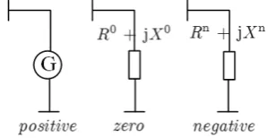
2.7.2. Distributed Generator Sequence Frame Model

The synchronous generator modeled in sequence frame consist of three part as shown in Figure 5. This model can be connected to phase-frame model with sequence-phase frame adaptor presented in 2.7.1.

Figure 5. Synchronous Generator Mode in Sequence Frame

DG can work in PQ or PV mode. The constraints’ equations of DG in PQ operating mode are written as

p p p p p

re re im im sp

U I +U I =P (48)

p p p p p

re im im re sp

U I U I Q

- + = (49)

n n n n n

re im re,

I R +I X =U (50)

n n n n n

re im im,

(7)

0 0 0 0 0

re im re,

I R +I X =U (52)

0 0 0 0 0

re im im.

I X +I R =U (53)

where Pspp and Qspp are positive sequence active and reactive power control target.

The constraints’ equations of DG in PV operating mode are written as

p p p p p

re re im im sp

U I +U I =P (54)

( ) ( )

_p 2 _p 2

( )

_p 2

re im sp

U + U = U (55)

n n n n n

re im re,

I R +I X =U (56)

n n n n n

re im im,

I X +I R =U (57)

0 0 0 0 0

re im re,

I R +I X =U (58)

0 0 0 0 0

re im im.

I X +I R =U (59)

where U_spp is positive sequence voltage magnitude control target. As Modelica uses Newton

algorithm to solve equations, voltage controlled equation (55) are easy to be coped with while

OpenDSS has difficulty which uses fixed point iteration method.

2.8. Step Voltage Regulator

One-phase step voltage regulator can be seen as a modified ideal transformer. The detail model can refer to kersting’s book [11]. The constraints equation are given by

b,1,re b,2,re,

U =kU (60)

b,1,im b,2,im,

U =kU (61)

b,1,re b,2,re,

kI = -I (62)

b,1,im b,2,im.

kI = -I (63)

(

)

b,2,re b,2,im b,2,re b,2,im

relay,re relay,im comp co

j j

j U U j _mp I I ,

U U R X

PT CT

+ +

+ = + + (64)

1 0.0065 ,

k = - ⋅tap (65)

2 2 2

relay relay,re relay,im,

U =U +U (66)

low,sp relay

relay low,sp

high,sp relay

relay high,sp ,

0.75 _,

, 0.75

U U

if U U

tap

U U

if U U

ì

-ïï

ï <

ïï

= í_ï

-ïï >

ïïî

(67)

where PT is potential transformer ratio, CT is current transformer ratio,

(

R_comp +jX_co_mp

)

denotes compensator impedance in Ohms which can be derived from compensator impedance in

Voltage. U_relay is relay voltage. U_low,sp and U_high,sp is minimum and maximum voltage of relay.

tap represents tap position of step voltage regulator.

2.9. Load

(8)

2.9.1. Constant Current Load

The power factor and current magnitude are constant for constant current load. The equations are given by

2 2 2

b,re b,im sp

I +I =I (68)

(

-Ub,re b,imI +Ub,im b,reI

)

P =

(

Ub,re b,reI +Ub,im b,imI

)

Q (69)

where P and Q are given active and reactive power. I_sp is specified current magnitude.

2.9.2. Constant Active and Reactive Power Load

The active and reactive power are constant for constant power load. The equations are given by

b,re b,re b,im b,im

P =U I +U I (70)

b,re b,im b,im b,re

Q= -U I +U I (71)

where P and Q are given active and reactive power.

2.10. Circuit Breaker

The open circuit breaker is modeled with zero current source while the closed circuit breaker is modeled with zero voltage source. This model is more accurate than small impedance branch model used in OpenDSS.

2.11. Short-circuit Analysis

Line to line or line to ground faults can be modeled as two node connected with zero voltage source. Taking one-phase to ground fault as example, the fault point branch equations are given by

b,re 0

U = (72)

b,im 0

U = (73)

In fact, the open circuit fault can be modelled with fault points connected with zero current source and equations are given by

b,re 0

I = (74)

b,im 0

I = (75)

3. Steady state analysis of Distribution Network

According to section 2, load flow and short circuit analysis can be both realized with Modelica. As Newton method is used to solve equations, the steady state analysis initialization is very important. Linear component such as voltage source, impedance branch, transformer are not needed to be initialized. While nonlinear components such as constant power load, constant current load, and distributed generators.

3.1. Constant Power Load Initialization

To assure convergence of steady state initialization, the constant power load is modelled as zero current source at initialization step.

b,re 0

I = (76)

b,im 0

I = (77)

3.2. Constant Current Load Initialization

(9)

b,re 0

I = (78)

b,im 0

I = (79)

3.3. PQ mode Synchronous Generator Initialization

Similar to constant power load, the synchronous generator is modelled as zero current source in positive sequence and equations are given by

p re 0

I = (80)

p im 0

I = (81)

3.4. PV mode Synchronous Generator Initialization

Considering the voltage control target, the synchronous generator is modelled as constant voltage source and equations are given by

p p

re sp

U =U (82)

p im 0

U = (83)

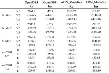
4. Results

The proposed program has been implemented on IEEE 4-bus, 13-bus test feeders. The load flow results are illustrated in Table 1, 2 and 3 and they are close to the IEEE given results. IEEE Distribution Test Feeder Task Force do not give the load flow program and the authors believe that the open source distribution steady state analysis platform is a supplement for active distribution system analysis. The IEEE 13-bus test feeder with 1-10 voltage controlled distributed generators are illustrated in Table 4. It can be seen that Newton-based ADN_Modelica has better ability of coping with PV mode DG than OpenDSS.

Table 1. The Load-Flow Results of IEEE 4 Node Test Feeder(GrY/GrY connection type for three-phase transformer).

OpenDSS Re

OpenDSS Im

ADN_Modelica

Re

ADN_Modelica

Im

Node 2 V1 V2 V3

7164.0 -3576.5 -3465.8

-12.5 -6145.0

6176.0

7163.73 -3575.18 -3462.43

-17.42 -6146.54

6178.46

Node 3 V1 V2 V3

2303.1 -1247.9 -924.05

-92.5 -1878.2

1999.8

2303.73 -1248.55 -923.00

-90.82 -1877.54

2000.20

Node 4 V1 V2 V3

2169.4 -1156.1 -406.1

-155.51 -1545.4 1787.4

2169.50 -1156.37 -409.24

-156.07 -1546.07

1788.33

Current 1-2

Ia Ib Ic

186.39 -306.92 42.04

-134.92 -159.09 453.15

186.35 -306.91

42.03

-134.91 -158.84 452.65

Current 3-4

Ia Ib Ic

558.69 -919.78 125.99

-404.42 -476.77 1358.2

558.60 -919.99

126.00

(10)

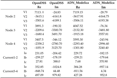
Table 2. The Load-Flow Results of IEEE 4 Node Test Feeder(GrY/D connection type for three-phase transformer). OpenDSS Re OpenDSS Im ADN_Modelica Re ADN_Modelica Im Node 2 V1 V2 V3 7113.0 -3615.1 -3501.6 -24.83 -6161.8 -6189.1 7119.15 -3617.91 -3506.11 -28.79 -6164.75 6193.38 Node 3 V1 V2 V3 3891.3 -2209.6 -1680.4 -190.32 -3300.70 3491.70 4047.52 -2132.30 -1915.18 -76.34 -3481.80 3557.81 Node 4 V1 V2 V3 3407.5 -2358.2 -1051.9 -346.12 -2780.70 3125.70 3595.30 -2293.40 -1301.80 -243.94 -2996.40 3240.40 Current1-2 Ia Ib Ic 231.05 -259.27 27.81 -204.42 -178.19 388.0 229.72 -239.21 7.68 -182.15 -179.64 370.90 Current3-4 Ia Ib Ic 352.85 -848.74 497.09 -1024.8 44.48 979.82 384.28 -811.56 427.28 -957.14 4.34 952.8

Table 3. The Load-Flow Results of IEEE 13 Node Test Feeder.

Node Phase OpenDSS vRe OpenDSS vIm ADN_Modelica vRe ADN Modelica vIm 650 A B C 2401.8 -1200.9 -1200.9 0 -2080 2080 2280.41 -1241.60 -1035.14 -120.62 -1958.43 2030.78 RG60 A B C 2551.9 -1260.9 -1283.4 0 -2184 2222.9 2432.44 -1306.95 -1111.55 -128.66 -2061.50 2180.71 632 A B C 2449.9 -1315.8 -1140.8 -106.54 -2128.8 2160.9 2309.72 -1348.43 -989.48 -219.77 -1993.0 2087.22 633 A B C 2442.6 -1315.3 -1137.5 -109.21 -2123.8 2155.6 2301.76 -1347.52 -986.50 -221.95 -1987.96 2081.28 XFXFM1 A B C 275.06 -150.98 -126.81 -15.522 -239.56 245.17 258.22 -154.45 -109.24 -28.35 -223.67 236.18 634 A B C 275.03 -150.98 -126.77 -15.52 -239.56 245.19 258.22 -154.45 -109.24 -28.35 -223.67 236.18

645 B C -1310.9 -1139.8 -2106.1 2156.3 -1342.20 -988.55 -1970.28 2083.01

646 B C -1311.6 -1138.9 -2100.6 2151.1 -1342.51 -1988.20 -1965.24 2077.97

(11)

C -1030.2 2110.4 -899.28 2003.19

680

A B C

2367.6 -1352.8 -1030.2

-219.64 -2136.6 2110.4

2210.10 -1372.08 -899.276

-318.24 -1985.67

2003.19

684 A C

2363 -1024.4

-220.04 2107.9

2209.13 -886.42

-318.93 1999.48

611 C -1017.2 2106.1 -883.05 1996.0 652 A 2349.8 -215.92 2205.11 -317.38

692

A B C

2367.6 -1352.8 -1030.1

-220.05 -2136.6 2110.2

2210.10 -1372.08 -889.28

-318.25 -1985.67

2003.19

675

A B C

2351 -1362.6 -1028.5

-228.86 -2137.2 2105.9

2189.68 -1367.78 -889.37

-321.95 -1985.68

1993.4

Table 4. Load Flow Iteration Number with different number of PV Generator

Platform 1 PV 5 PV 10 PV

OpenDSS 8 iterations divergence Divergence ADN_Modelica 5 iterations 5 iterations 5 iterations

5. Discussion

The proposed program can deal with phase-sequence coupled model and can give more accurate results than OpenDSS when floating network exists. The reason is that OpenDSS adds anti-floating impedance branch to Delta connection load which breaks the original KCL constraints as depicted in Figure 6. Another reason is that closed circuit breaker is modelled as small impedance branch in OpenDSS which will bring small error.

Figure 6. Anti-floating Method in OpenDSS

6. Conclusions

The proposed open source program can be downloaded from [14] and it has several contributions:

(1)It can cope with sequence-phase coupled active distribution network. In the future, voltage source converters, doubly-fed generator will be added to this platform. Open source electromagnetic transient and electromechanical transient simulation are under development. The steady state analysis ADN_Modelica will be an initialization program for transient simulation.

(12)

(3)Newton method is used and PV mode generators can be easily handled in ADN_Modelica. Finally this is an open source program and it will help researchers and educators to implement further modelling, optimization and control experiments of active distribution network.

Acknowledgments: This work was supported by State Key Laboratory foundation project SKLD16KZ08 and State grid Fujian electric power company Economic institute of technology science and technology project SGFJJY00GHWT1600081.

Author Contributions: Yuntao Ju conceived and designed the experiments; Fuchao Ge, Yi Lin, Jing Wang performed the experiments.

Conflicts of Interest: The authors declare no conflict of interest.

References

1. F. Milano, L. Vanfretti, J. C. Morataya. An Open Source Power System Virtual Laboratory: The PSAT Case and Experience. IEEE Transactions on Education2008, 51, pp. 17–23, DOI:10.1109/TE.2007.893354.

2. R. D. Zimmerman, C. E. Murillo-Sanchez, R. J. Thomas, MATPOWER: Steady-State Operations, Planning, and Analysis Tools for Power Systems Research and Education, IEEE Transactions on Power Systems 2011,

26, pp. 12–19,DOI: 10.1109/TPWRS.2010.2051168.

3. R. C. Dugan , T. E. McDermott, An open source platform for collaborating on smart grid research, IEEE Power and Energy Society General Meeting2011, pp. 1–7, DOI: 10.1109/PES.2011.6039829.

4. P. A. N. Garcia, J. L. R. Pereira, S. Carneiro, M. P. Vinagre, F. V. Gomes, Improvements in the representation of PV buses on three-phase distribution power flow, IEEE Transactions on Power Delivery2004, 19, pp. 894– 896, DOI: 10.1109/TPWRD.2003.820414.

5. D. P. Chassin, K. Schneider, C. Gerkensmeyer, GridLAB-D: An open-source power systems modeling and simulation environment, IEEE/PES Transmission and Distribution Conference and Exposition2008, pp. 1–5, DOI: 10.1109/TDC.2008.4517260.

6. Y. Ju, W. Wu, B. Zhang, H. Sun, An Extension of FBS Three-Phase Power Flow for Handling PV Nodes in Active Distribution Networks, IEEE Transactions on Smart Grid 2014, 5, pp. 1547–1555, DOI: 10.1109/TSG.2014.2310459.

7. O. Enge, C. Claub, P. Schneider, P. Schwarz, M. Vetter, S. Schwunk, Quasi-stationary AC analysis using phasor description with Modelica., 5th Int. Modelica Conf.2006, pp. 579–588.

8. M. Z. Kamh, component modeling and three-phase power flow analysis for active distribution systems. PhD Thesis, University of Toronto, 2011.

9. T. E. McDermott, A test feeder for DG protection analysis, IEEE/PES Power Systems Conference and Exposition (PSCE)2011, pp. 1–7, DOI: 10.1109/PSCE.2011.5772608.

10. H. Elmqvist and S. E. Mattsson, Modelica—The Next Generation Modeling Language An International Design Effort, Proceedings of the 1st World Congress on System Simulation (WCSS’97), 1997.

11. William H. Kersting, Distribution System Modeling and Analysis, Third Edition, Publisher: CRC Press, Boca Raton.

12. Distribution Test Feeders. Available online: https://ewh.ieee.org/soc/pes/dsacom/testfeeders/ (accessed on 12 Sep. 2016).

13. ADN_Modelica. Available online: https://github.com/eetonyju/ ADN_Modelica (accessed on 12 Sep. 2016).