Application of a failure driven test profile in random testing

(1)

Application of a Failure Driven Test Profile in Random Testing

Tsong Yueh Chen, Member, IEEE, Fei-Ching Kuo, Member, IEEE, and Huai Liu

Faculty of Information and Communication Technologies

Swinburne University of Technology

Hawthorn, Victoria 3122, Australia

{

tchen, dkuo, hliu

}

@ict.swin.edu.au

Abstract

Random testing techniques have been extensively used in reliability assessment, as well as in debug testing. When used to assess software reliability, random testing selects test cases based on an operational profile; while in the context of debug testing, random testing often uses a uniform distribution. However, generally neither an operational profile nor a uniform distribution is chosen from the perspective of max-imizing the effectiveness of failure detection. Adaptive random testing has been proposed to enhance the failure detection capability of random testing by evenly spreading test cases over the whole input domain. In this paper, we propose a new test profile, which is different from both the uniform distribution, and operational profiles. The aim of the new test profile is to maximize the effectiveness of failure detection. We integrate this new test profile with some existing adaptive random testing algorithms, and develop a family of new random testing algorithms. These new algorithms not only distribute test cases more evenly, but also have better failure detection capabilities than the corresponding original adaptive random testing algorithms. As a consequence, they perform better than the pure random testing.

(2)

Acronym1

RT Random Testing

ART Adaptive Random Testing

FSCS-ART Fixed-Sized-Candidate-Set Adaptive Random Testing RRT Restricted Random Testing

ART-DNC Adaptive Random Testing with Dynamic Non-Uniform Candidate Distribution pdf Probability Density Function

PDF Probability Distribution Function

Notation

E The set of all executed test cases

I The input domain

N The dimension of input domain ND N-dimension, where N=1,2,3,4,· · · | · | The size of a set

θ The failure rate of a program

F-measure The expected number of test cases required to detect the first program failure FRT F-measure of random testing

FART F-measure of adaptive random testing ART F-ratio FART

FRT

(3)

1. Introduction

Random testing (RT) is a standard software testing technique which simply generates test cases

(that is, program inputs for testing) at random from the whole input domain (that is, the set of all possible inputs for the program under test) [15], [21]. RT has been widely used for assessing soft-ware reliability [14], [23], where test cases are often selected according to an operational profile. The operational profile refers to a probability distribution, over the input domain, which charac-terizes how a program is operated by end-users [20]. Another application of RT is debug testing, which aims at detecting software failures so that program bugs can be removed, and thus software reliability can be improved [13]. When used as a debug testing method, RT often selects test cases based on a uniform distribution; that is, all program inputs have the same probability to be selected as test cases, to ensure that every possible bug could be detected.

Inputs that cause the program under test to exhibit failure behaviors are known as failure-causing inputs. A testing method is said to detect a failure if it picks a failure-causing input as a test case.

(4)

other inputs. Briefly speaking, both test profiles for RT are not failure oriented, and hence are not expected to ensure an optimal failure detection capability for RT. This lack has motivated us to investigate whether different test profiles can enhance the effectiveness of RT.

Several studies [1], [2], [12], [25] have independently made a common observation that failure-causing inputs tend to cluster into contiguous regions (known as failure regions [1]) in the input domain. Chen et al. [7] have attempted to improve the effectiveness of RT by means of this characteristic of failure-causing inputs. Their intuition is that, if a test case t does not reveal any software failure, then an input that is away from t is more likely to cause a failure than t’s neighbors. Based on such an intuition, they proposed a novel approach, namely adaptive random testing (ART), which not only randomly selects, but also more evenly spreads test cases over the input domain. Various algorithms have been developed to implement the basic “even spread” intuition of ART, such as fixed-sized-candidate-set ART (FSCS-ART) [7], restricted random testing (RRT) [3], and lattice-based ART [17]. Most ART algorithms consist of two independent processes. One process (known as candidate generation process) randomly generates program inputs as test case candidates, or briefly candidates. The other process (known as test case identification process)

applies some criteria to identify test cases among these candidates to ensure an even spread of test cases across the input domain. Because ART was originally proposed as a debug testing method, the random generation of candidates has always been conducted according to a uniform distribution.

(5)

all used the uniform distribution as the test profile for the candidate generation process. However, as mentioned before, such a uniform distribution is not chosen specifically to help improve the effectiveness of RT. We are motivated to look at what test profile can be used to enhance the failure detection capability of RT/ART. In this paper, we propose to develop another test profile, which is different from the uniform distribution, and the operational profile, for the candidate generation process in ART. Our approach is to design a test profile for the candidate generation process such that the test case identification process would deliver a more even distribution of test cases, and consequently, a likely improvement of the failure detection capability. We call such a profile as failure driven test profile. We conduct investigations on two particular ART algorithms:

FSCS-ART [7], and RRT [3].

Section 2 introduces the background information on FSCS-ART, and RRT. Some concepts used in this paper are also discussed in this section. In Section 3, we investigate how to select a test profile that can be used to guide the candidate generation in FSCS-ART, and RRT, while keeping the test case identification criteria unchanged. The resultant new algorithms are evaluated via some simulations, whose results are also reported in this section. Section 4 concludes the paper. The appendix contains details of some calculations.

2. Background

(6)

2.1. Fixed-sized-candidate-set adaptive random testing

Fixed-sized-candidate-set ART (FSCS-ART) [7] makes use of two sets of test cases: the ex-ecuted set E ={e1,e2,· · ·,en}, which contains the executed test cases; and the candidate set C ={c1,c2,· · ·,ck}, which contains k randomly generated candidates. A candidate cb will be chosen as the next test case if for all j=1,2,· · ·,k,

n min

i=1 dist(cb,ei)≥

n min

i=1 dist(cj,ei), (1)

where dist is the Euclidean distance between two points. The details of the FSCS-ART algorithm can be found in [7]. Although the performance of FSCS-ART improves with the increase of k, any k>10 will not significantly improve the effectiveness of FSCS-ART [7]. Therefore, in this paper, we will use FSCS-ART where k has a value of 10.

2.2. Restricted random testing

Restricted random testing (RRT) [3] creates an exclusion region around each element of E. Only

(7)

3.3, and 6.4 for RRT in 1D, 2D, 3D, and 4D spaces, respectively, as suggested in [3].

2.3. Failure detection capability of adaptive random testing

The F-measure, the expected number of test cases required to detect the first software failure, has been used for measuring the failure detection capability of ART. This paper will follow all previous studies of ART in using the F-measure as the effectiveness metric. Readers may refer to [8] for an explanation for why the F-measure is more appropriate than other metrics in evaluating ART. In this paper, F-measures of RT, and ART are denoted by FRT, and FART, respectively. The ART F-ratio, the ratio between FART and FRT, is used to show the improvement of ART over RT.

Generally speaking, failure-causing inputs determine two basic features of a faulty program. One feature is the failure rate (denoted by θ), which refers to the ratio between the number of failure-causing inputs, and the number of all possible inputs. The failure pattern, the other ba-sic feature, refers to the failure regions together with their distribution over I. Both θ, and the failure pattern are unknown before testing, although they are fixed after coding. Theoretically, FRT =1/θ when test cases are randomly selected according to uniform distribution, and with replacement. Obviously, a theoretical analysis of FART is extremely difficult, and thus previous studies of ART [4], [5], [6] have estimated FART via simulations, using the basic procedure as follows.

(8)

is repeated for a sufficiently large number (S) of times to ensure that the average value of F-counts can be regarded as a reliable estimate for FART within a specified confidence level, and an accuracy range (details of deciding S can be found in [7]). In this paper, the default values of confidence level, and accuracy range are set as 95%, and±5%, respectively.

Previous studies [4], [6] showed that FSCS-ART, and RRT perform best when failure-causing inputs are well clustered into one single compact region. However, their failure detection capabil-ities deteriorate asθ becomes higher, N becomes higher, the failure region becomes less compact, or the number of failure regions becomes larger.

2.4. Test case distribution of adaptive random testing

Because the basic intuition of ART is the even spread of test cases, some research [4], [19] has been conducted to measure how evenly ART algorithms spread test cases from different perspec-tives. In [19], the test case distributions of various ART algorithms were coarsely described by some 2D spatial distribution graphs. A more precise approach for measuring test case distributions was proposed by Chen et al. [4], where some distribution metrics were employed to measure the evenness of test case distribution. Among these metrics, discrepancy, and dispersion are two com-monly used measurement metrics for the equidistribution of sample points. Discrepancy indicates the maximal difference of points’ densities for various regions in I, while dispersion indicates the size of the largest empty spherical region (containing no point) in I. Smaller discrepancy or smaller dispersion implies better equidistribution of sample points.

(9)

smaller. As mentioned in Section 2.3, FSCS-ART, and RRT have poor failure detection capabilities for high N, or highθ cases. Such a correlation between the ART effectiveness, and the test case distribution has motivated us to look at how to enhance the failure detection capability of ART through the improvement of the evenness of test case distribution.

3. Adaptive Random Testing using a Non-Uniform Distribution as a Test Profile

As mentioned before, neither the uniform distribution (for debug testing), nor the operational profile (for reliability assessment) is designed specifically to help RT achieve an optimal failure detection capability. ART improves the failure detection capability of RT by evenly spreading random test cases. There are two independent processes in most ART algorithms: the candidate generation process, which ensures the randomness of test cases; and the test case identification process, which ensures the even spread of random test cases. All previous studies of ART were focused on the test case identification process, while the candidate generation process always used a uniform distribution, just like RT as a debug testing method. This study attempts to investigate whether applying a different test profile in the candidate generation process can enhance the even spread of test cases, aiming at improving the failure detection capability of RT/ART.

(10)

3.1. Describing the tc-bias of an adaptive random testing algorithm

If points are equidistributed, each coordinate of them will be equidistributed. Hence, if the projections of points in any dimension are non-equidistributed, we can say that these points are not equidistributed. Therefore, if we check just one coordinate of the test cases selected by an ART algorithm, and find any bias, then we may judge that the ART algorithm has tc-bias.

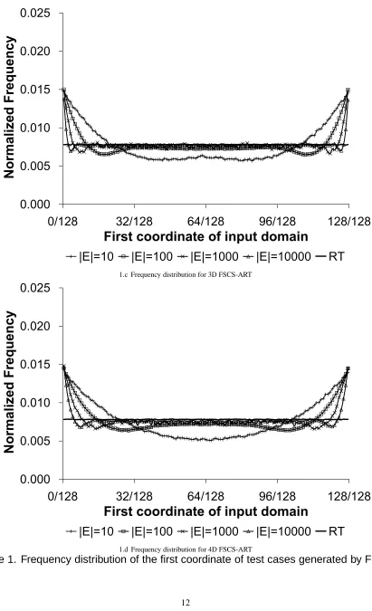
Our method for measuring the tc-bias is as follows. Suppose that I is a unit square such that each dimension of I has the range of value as[0,1). We choose a certain coordinate, say the 1st coordinate, and divide it into m equal-sized subdomains,[0,1/m),[1/m,2/m),· · ·,[(m−1)/m,1). Then, a set of test cases are generated using an ART algorithm. For each subdomain, we record the number of test cases whose 1st coordinates are inside this subdomain. The normalized frequency of points inside each subdomain is then calculated. Such a process will be repeated for a sufficient number of times so that reliable average values of frequencies are obtained within a 95% confi-dence level, and a±5% accuracy range. Based on the values of the collected average normalized frequencies for these m subdomains, we calculate two more statistics: i) the standard deviation of these m average normalized frequencies, denoted by stdev; and ii) the difference between the maximal and minimal values of these m average normalized frequencies, denoted by max−min. The smaller max−min and stdev are, the lower tc-bias an ART algorithm has.

(11)

0.000

0.005

0.010

0.015

0.020

0.025 0/128

32/128

64/128

96/128

128/128

First coordinate of input domain

Norma

lized

Freque

ncy

|E|=10

|E|=100

|E|=1000

|E|=10000

RT

1.a Frequency distribution for 1D FSCS-ART

0.000

0.005

0.010

0.015

0.020

0.025 0/128

32/128

64/128

96/128

128/128

First coordinate of input domain

Norma

lized

Freque

ncy

|E|=10

|E|=100

|E|=1000

|E|=10000

RT

(12)

0.000

0.005

0.010

0.015

0.020

0.025 0/128

32/128

64/128

96/128

128/128

First coordinate of input domain

Norma

lized

Freque

ncy

|E|=10

|E|=100

|E|=1000

|E|=10000

RT

1.c Frequency distribution for 3D FSCS-ART

0.000

0.005

0.010

0.015

0.020

0.025 0/128

32/128

64/128

96/128

128/128

First coordinate of input domain

Norma

lized

Freque

ncy

|E|=10

|E|=100

|E|=1000

|E|=10000

RT

1.d Frequency distribution for 4D FSCS-ART

(13)

testing methods) are summarized in Table 1. In Fig. 1, the x-, and y-axes denote the locations of the first dimension’s subdomains, and the normalized frequencies of test cases inside these subdomains, respectively. We found that the test case distribution of RT is always uniform no matter how many test cases were generated, which is theoretically expected. Therefore, we only plot the frequency distribution of RT where |E|=10000. Note that, although RT does not have any tc-bias, that does not mean that RT is better than ART in terms of the F-measure.

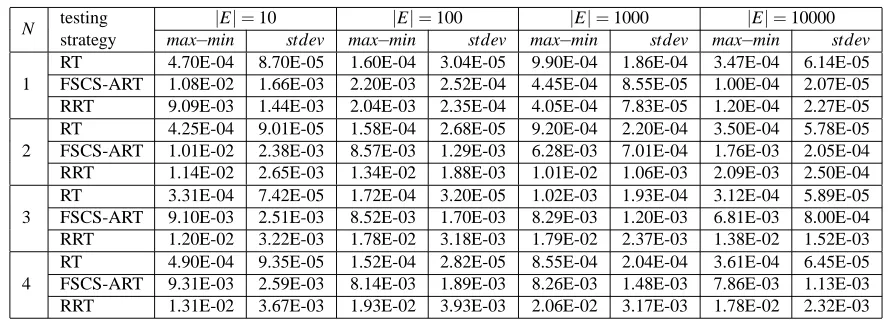
Table 1. Values ofmax−min, andstdevfor FSCS-ART, RRT, and RT

N testing |E|=10 |E|=100 |E|=1000 |E|=10000

strategy max−min stdev max−min stdev max−min stdev max−min stdev

1

RT 4.70E-04 8.70E-05 1.60E-04 3.04E-05 9.90E-04 1.86E-04 3.47E-04 6.14E-05

FSCS-ART 1.08E-02 1.66E-03 2.20E-03 2.52E-04 4.45E-04 8.55E-05 1.00E-04 2.07E-05 RRT 9.09E-03 1.44E-03 2.04E-03 2.35E-04 4.05E-04 7.83E-05 1.20E-04 2.27E-05

2

RT 4.25E-04 9.01E-05 1.58E-04 2.68E-05 9.20E-04 2.20E-04 3.50E-04 5.78E-05

3

RT 3.31E-04 7.42E-05 1.72E-04 3.20E-05 1.02E-03 1.93E-04 3.12E-04 5.89E-05

4

RT 4.90E-04 9.35E-05 1.52E-04 2.82E-05 8.55E-04 2.04E-04 3.61E-04 6.45E-05

The experimental data of Table 1, and Fig. 1 show that both FSCS-ART, and RRT have certain tc-biases, and the tc-biases become higher with the increase of N, as well as with the decrease of

|E|. Further investigation of the frequency distribution graphs show that points from the boundary

part of I have higher probabilities to be selected as test cases than those from the central part of I. Moreover, all frequency distributions are symmetric with respect to the center of I.

(14)

3.2. Designing a non-uniform distribution as a test profile

To offset the tc-biases of FSCS-ART, and RRT, the new test profile for the candidate generation process should have the following essential features.

• The probability distribution in the test profile must be dynamic throughout the testing process;

that is, the test profile should be changeable as E changes because the amount of tc-bias to be offset varies as E changes.

• The elements in the central part must have a higher probability of being selected as candidates

than the elements in the boundary part because the candidates from the central part have a lower probability of being selected as the next test case.

• The probability distribution must be symmetric with respect to the center of I because the

distribution of test cases is also symmetric with respect to the center of I.

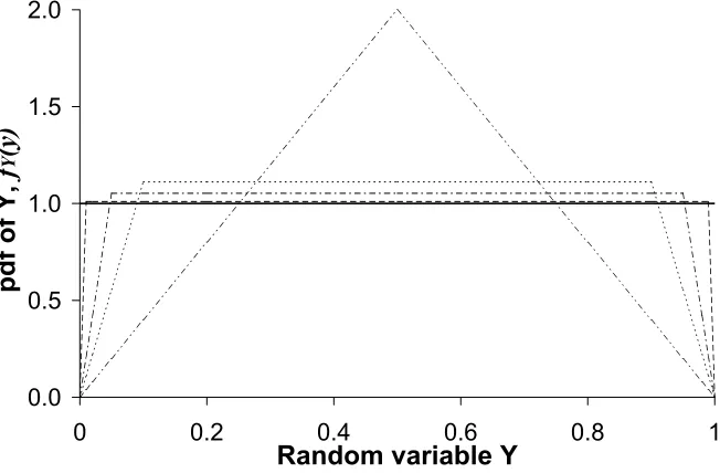
Many non-uniform distributions have the above properties. A simple example is a linear com-bination of two uniform-distributed random variables.

Y =αX1+ (1−α)X2, (2)

where 0≤α ≤0.5. X1, and X2 are two random variables which are both uniformly distributed in

[0,1). The probability density function (pdf) of Y , denoted by fY(y), is

fY(y) =

              

             

0 , when y<0 or y≥1 y

α(1−α), when 0≤y<α

1

(1−α) , when α ≤y<1−α

1−y

α(1−α), when 1−α ≤y<1

(15)

Appendix A describes how to derive fY(y), and Fig. 2 shows distributions of Y for variousα.

0.0 0.5 1.0 1.5 2.0

0 0.2 0.4 0.6 0.8 1

Random variable Y

pdf of

Y,

f

Y

(y)

Figure 2. The probability density function ofY.

3.3. Our approach

We propose to generate candidates according to 2 instead of the uniform distribution; as a result, more candidates are likely to be chosen from the center of I than from the edge. The parameterα in 2, and 3 decides how likely candidates are to be selected from the center. In each dimension, for each round of test case selection,α is dynamically chosen as follows.

For ease of illustration, assume that each dimension of I has the value range[0,1), and is equally divided into two subranges: the central subrange consisting of [0.25,0.75); and the boundary subrange consisting of[0,0.25), and[0.75,1). We then define the following two parameters.

• The normalized ratio of the lth coordinate of E (the set of all already executed test

cases) being located in the boundary subrange of the lth dimension of I (denoted by

(16)

co-ordinates are denoted by e1l,e2l,· · ·,enl, respectively, where 0≤eil<1 (i=1,2,· · ·,n). We define E_tcl₋_boundary ={eil|0≤eil<0.25 or 0.75≤eil<1}. p_tcl ₋_boundary is defined as

p_tcl ₋_boundary =|E l

tc−boundary|

|E| (4)

Note that the values of pl_tc₋_boundary for FSCS-ART, and RRT are usually larger than 0.5.

• The probability of the lth coordinate of a random candidate to be selected from the

central subrange of the lth dimension of I (denoted by P_canl ₋_central). For a candidate c

randomly generated according to 2, its lth coordinate is denoted by cl, where 0≤cl <1. P_canl ₋_central is defined as the probability of 0.25 ≤cl < 0.75. The value of P_canl ₋_central is decided byα in 2, and 3, as follows.

P_canl ₋_central=    

  

1

2(1−α) , when 0≤α<0.25

1− 1

16α(1−α), when 0.25≤α ≤0.5

(5)

Appendix B contains the deduction of 5. Note that P_canl ₋_centralis within[0.5,0.75].

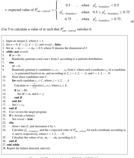
Our approach uses the following three steps to decide the value ofα for each dimension, suc-cessively after each new test case is selected.

1. For each coordinate, measure pl_tc₋_boundary along the testing process, where l=1,2,· · ·,N.

(17)

s−expected value of P_canl ₋_central=     

   

0.5 , when pl_tc₋_boundary<0.5

pl_tc₋_boundary, when 0.5≤p_tcl ₋_boundary ≤0.75 0.75 , when pl_tc₋_boundary>0.75.

(6) 3. Use 5 to calculate a value ofα such that P_canl ₋_central satisfies 6.

1. Input an integer k, where k>1.

2. Set n=0, E={}, C={}, and reveal = false.

3. Setα1=α2=· · ·=αN=0.5, where N denotes the dimension of I.

4. while (not reveal) 5. if (n=0)

6. Randomly generate a test case t from I, according to a uniform distribution. 7. else

8. M=0.

9. Randomly generate k candidates c1,c2,· · ·,ckfrom I, where each coordinate cjl of a candidate cjis generated based onαl, and according to 2, j=1,2,· · ·,k, and l=1,2,· · ·,N.

10. Store these candidates into C.

11. for each candidate cj∈C, where j=1,2,· · ·,k

12. Calculate m=minn

i=1dist(cj,ei), where ei∈E.

13. if (m>M)

14. Set M=m, and b=j.

15. end if 16. end for 17. Set t=cb.

18. end if

19. Use t to test the target program. 20. if (t reveals a failure)

21. Set reveal = true. 22. else

23. Store t into E, and increment n by 1.

24. Calculate pl_tc₋_boundary, and the s-expected value of P_canl ₋_centralfor each coordinate according to 4, and 6, respectively, where l=1,2,· · ·,N.

25. Calculate the values ofα1,α2,· · ·,αN according to 5.

26. end if 27. end while

28. Report the failure detected, and exit.

Figure 3. The algorithm of FSCS-ART-DNC.

(18)

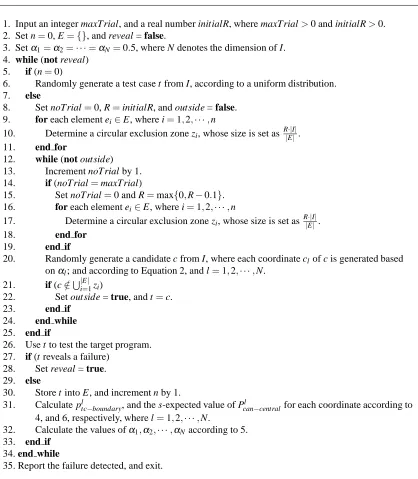
1. Input an integer maxTrial, and a real number initialR, where maxTrial>0 and initialR>0. 2. Set n=0, E={}, and reveal = false.

3. Setα1=α2=· · ·=αN=0.5, where N denotes the dimension of I.

4. while (not reveal) 5. if (n=0)

6. Randomly generate a test case t from I, according to a uniform distribution. 7. else

8. Set noTrial=0, R=initialR, and outside = false.

9. for each element ei∈E, where i=1,2,· · ·,n

10. Determine a circular exclusion zone zi, whose size is set as R_|·|_EI_||.

11. end for

12. while (not outside) 13. Increment noTrial by 1. 14. if (noTrial=maxTrial)

15. Set noTrial=0 and R=max{0,R−0.1}. 16. for each element ei∈E, where i=1,2,· · ·,n

17. Determine a circular exclusion zone zi, whose size is set asR_|·|_EI_||.

18. end for

19. end if

20. Randomly generate a candidate c from I, where each coordinate clof c is generated based

onαl; and according to Equation 2, and l=1,2,· · ·,N.

21. if (c∈/S|E|

i=1zi)

22. Set outside = true, and t=c.

23. end if 24. end while 25. end if

26. Use t to test the target program. 27. if (t reveals a failure)

28. Set reveal = true. 29. else

30. Store t into E, and increment n by 1.

31. Calculate pl_tc₋_boundary, and the s-expected value of P_canl ₋_centralfor each coordinate according to 4, and 6, respectively, where l=1,2,· · ·,N.

32. Calculate the values ofα1,α2,· · ·,αN according to 5.

33. end if 34. end while

35. Report the failure detected, and exit.

(19)

there is a family of software testing methods, namely statistical testing [11],[24], which also ran-domly generates program inputs according to some non-uniform distributions, which are in turn based on some criteria of either the program structure or the functionality. Although our approach also generates random inputs non-uniformly, our purpose is to distribute test cases more evenly, and hence to detect software failures more effectively, without aiming at achieving other criteria (such as program function or structure).

We propose two ART-DNC algorithms, namely FSCS-ART-DNC, and RRT-DNC, as shown in Figs. 3, and 4, respectively. As a reminder, the test case identification processes of the new ART-DNC algorithms remain the same as those of their counterparts. The aim of using the non-uniform distribution in the candidate generation processes is to improve the failure detection capability of ART, so we call this non-uniform profile a failure driven test profile.

3.4. Test case distributions of new algorithms

Prior to further research, we must check whether using the non-uniform test profile for candidate generation results in a more even spread of test cases. Only then will it make sense to evaluate the failure detection capabilities of ART-DNC. We therefore repeated the simulations in Section 3.1, but instead using FSCS-ART-DNC, and RRT-DNC. The simulations showed similar frequency dis-tributions of test cases for FSCS-ART-DNC, and RRT-DNC. Therefore, we only plot the frequency distribution graph of FSCS-ART-DNC in Fig. 5. For ease of comparison, we replot the test case distribution of pure RT (the same as that in Fig. 1), which is expected to be uniform. The values of max−min, and stdev for FSCS-ART-DNC,and RRT-DNC are summarized in Table 2.

(20)

0.000

0.005

0.010

0.015

0.020

0.025 0/128

32/128

64/128

96/128

128/128

First coordinate of input domain

Norma

lized

Freque

ncy

|E|=10

|E|=100

|E|=1000

|E|=10000

RT

5.a Frequency distribution for 1D FSCS-ART-DNC

0.000

0.005

0.010

0.015

0.020

0.025 0/128

32/128

64/128

96/128

128/128

First coordinate of input domain

Norma

lized

Freque

ncy

|E|=10

|E|=100

|E|=1000

|E|=10000

RT

(21)

0.000

0.005

0.010

0.015

0.020

0.025 0/128

32/128

64/128

96/128

128/128

First coordinate of input domain

Norma

lized

Freque

ncy

|E|=10

|E|=100

|E|=1000

|E|=10000

RT

5.c Frequency distribution for 3D FSCS-ART-DNC

0.000

0.005

0.010

0.015

0.020

0.025 0/128

32/128

64/128

96/128

128/128

First coordinate of input domain

Norma

lized

Freque

ncy

|E|=10

|E|=100

|E|=1000

|E|=10000

RT

5.d Frequency distribution for 4D FSCS-ART-DNC

(22)

tc-biases of FSCS-ART, and RRT.

Table 2. Values ofmax−min, andstdevfor FSCS-ART-DNC, and RRT-DNC

N testing |E|=10 |E|=100 |E|=1000 |E|=10000

strategy max−min stdev max−min stdev max−min stdev max−min stdev

1 FSCS-ART-DNC 7.63E-03 1.16E-03 1.64E-03 1.52E-04 7.00E-04 9.52E-05 3.03E-04 3.71E-05 RRT-DNC 5.50E-03 9.03E-04 1.42E-03 1.30E-04 5.70E-04 8.19E-05 2.29E-04 3.03E-05

We further investigate the test case distribution of ART-DNC algorithms by repeating the simu-lations in [4] on FSCS-ART-DNC, and RRT-DNC. They distribute their test cases similarly. There-fore, we only plot discrepancy, and dispersion for FSCS-ART-DNC, with previous FSCS-ART’s data for ease of comparison, in Figs. 6, and 7, respectively. The simulations results show that ART-DNC algorithms usually have smaller values of discrepancy than the original ART algorithms, and they have similar values of dispersion.

In summary, the experimental results have demonstrated that our approach achieves a more even spread of test cases. By using such a simple failure driven test profile (linear combination of two uniform-distributed variables) for candidate generation, we are able to achieve a more even test case distribution of ART.

3.5. Failure detection capabilities of new algorithms

(23)

0.00 0.01 0.02 0.03 0.04 0.05

0 2000 4000 6000 8000 10000

|E|

Dis

crep

ancy

FSCS-ART FSCS-ART-DNC

6.a Discrepancy in 1D space

0.00 0.01 0.02 0.03 0.04 0.05 0.06 0.07 0.08

0 2000 4000 6000 8000 10000

|E|

Dis

crep

ancy

6.b Discrepancy in 2D space

0.01 0.02 0.03 0.04 0.05 0.06 0.07 0.08 0.09

0 2000 4000 6000 8000 10000

|E|

Dis

crep

ancy

6.c Discrepancy in 3D space

0.01 0.02 0.03 0.04 0.05 0.06 0.07 0.08

0 2000 4000 6000 8000 10000

|E|

Dis

crep

ancy

6.d Discrepancy in 4D space

Figure 6. Comparison of discrepancy between FSCS-ART-DNC, and FSCS-ART.

0.00 0.01 0.02

0 2000 4000 6000 8000 10000

|E|

Dispers

ion

7.a Dispersion in 1D space

0.00 0.02 0.04 0.06 0.08 0.10 0.12 0.14

0 2000 4000 6000 8000 10000

|E|

Dispers

ion

(24)

0.05 0.10 0.15 0.20 0.25 0.30

0 2000 4000 6000 8000 10000

|E|

Dispers

ion

7.c Dispersion in 3D space

0.10 0.15 0.20 0.25 0.30 0.35 0.40 0.45

0 2000 4000 6000 8000 10000

|E|

Dispers

ion

7.d Dispersion in 4D space

Figure 7. Comparison of dispersion between FSCS-ART-DNC, and FSCS-ART.

• N: 1, 2, 3, and 4.

• θ: 0.75, 0.5, 0.25, 0.1, 0.075, 0.05, 0.025, 0.01, 0.0075, 0.005, 0.0025, 0.001, 0.00075,

0.0005, 0.00025, 0.0001, 0.000075, and 0.00005.

• Failure pattern: a single square/cubic failure region is randomly placed inside I.

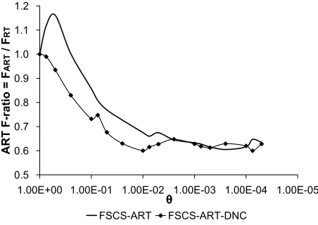
The results of the simulations are reported in Figs. 8, and 9. For ease of comparison, the simu-lation results of FSCS-ART, and RRT under the same experimental settings are also plotted.

Based on the experimental data, we have the following observations.

• Compared with the original FSCS-ART, and RRT algorithms, both FSCS-ART-DNC, and

RRT-DNC algorithms have better or similar failure detection capabilities. On average, in 1D, 2D, 3D, and 4D spaces, FSCS-ART-DNC improves the failure detection capability of FSCS-ART by 1.65%, 6.66%, 10.35%, and 15.00%, respectively; and the performance im-provements of RRT-DNC over RRT are 0.73%, 4.00%, 10.84%, and 17.38%, respectively.

• The higher N, or higherθ, the better the performance improvement of ART-DNC algorithms

(25)

0.5 0.6 0.7 0.8 0.9 1.0 1.1 1.00E-05 1.00E-04 1.00E-03 1.00E-02 1.00E-01 1.00E+00 ART F-r atio = F ART / F RT FSCS-ART FSCS-ART-DNC

8.a FSCS-ART-DNC vs. FSCS-ART in 1D space

0.5 0.6 0.7 0.8 0.9 1.0 1.1 1.2 1.00E-05 1.00E-04 1.00E-03 1.00E-02 1.00E-01 1.00E+00 ART F-r atio = F ART / F RT FSCS-ART FSCS-ART-DNC

8.b FSCS-ART-DNC vs. FSCS-ART in 2D space

0.6 0.7 0.8 0.9 1.0 1.1 1.2 1.3 1.4 1.00E-05 1.00E-04 1.00E-03 1.00E-02 1.00E-01 1.00E+00 ART F-r atio = F ART / F RT FSCS-ART FSCS-ART-DNC

8.c FSCS-ART-DNC vs. FSCS-ART in 3D space

0.7 0.8 0.9 1.0 1.1 1.2 1.3 1.4 1.5 1.6 1.7 1.00E-05 1.00E-04 1.00E-03 1.00E-02 1.00E-01 1.00E+00 ART F-r atio = F ART / F RT FSCS-ART FSCS-ART-DNC

8.d FSCS-ART-DNC vs. FSCS-ART in 4D space

Figure 8. Comparison of failure detection capability between ART-DNC, and FSCS-ART 0.5 0.6 0.7 0.8 0.9 1.0 1.00E-05 1.00E-04 1.00E-03 1.00E-02 1.00E-01 1.00E+00 ART F-r atio = F ART / F RT RRT RRT-DNC

9.a RRT-DNC vs. RRT in 1D space

0.5 0.6 0.7 0.8 0.9 1.0 1.1 1.00E-05 1.00E-04 1.00E-03 1.00E-02 1.00E-01 1.00E+00 ART F-r atio = F ART / F RT RRT RRT-DNC

(26)

0.6 0.7 0.8 0.9 1.0 1.1 1.2 1.3 1.4 1.5

1.00E-05 1.00E-04

1.00E-03 1.00E-02

1.00E-01 1.00E+00

ART

F-r

atio

=

F

ART

/ F

RT

RRT RRT-DNC

9.c RRT-DNC vs. RRT in 3D space

0.7 1.0 1.3 1.6 1.9 2.2

1.00E-05 1.00E-04

1.00E-03 1.00E-02

1.00E-01 1.00E+00

ART

F-r

atio

=

F

ART

/ F

RT

RRT RRT-DNC

9.d RRT-DNC vs. RRT in 4D space

Figure 9. Comparison of failure detection capability between RRT-DNC, and RRT

detection capabilities; but in 4D space, the performance of FSCS-ART-DNC is 14.64%, or 40.03% better than FSCS-ART whenθ is 0.0025, or 0.25, respectively.

Both ART-DNC algorithms can distribute their test cases more evenly than the original ART algorithms, so it is intuitively expected that the former have better failure detection capabilities than the latter. Thus, the first observation is consistent with our expectation. It has been shown in [4] that the test case distributions of the original algorithms are less even when eitherθ or N is higher. Therefore, it is understandable to have the second observation that the new ART-DNC algorithms outperform their counterparts more under the situations of higherθ, and higher N.

(27)

• N: 2, 3, and 4.

• θ: 0.005, and 0.001.

• Experiment to investigate the impact of the compactness of failure region on the failure

de-tection capability.

– Failure pattern: a single rectangular/cuboid region is randomly placed inside I. The ratios

among edge lengths of the rectangular/cuboid region are 1 :γ, 1 :γ :γ, and 1 :γ :γ :γ in 2D, 3D, and 4D spaces, respectively, whereγ≥1.

– γ: 1, 4, 7, 10, 20, 30, 40, 50, 60, 70, 80, 90, and 100. As explained in [6], the largerγ is, the less compact the failure region is.

• Experiment to investigate the impact of the number of failure regions on the failure detection

capability.

– Failure pattern: a number of square/cubic regions are randomly placed inside I. Suppose

that there are n failure regions, denoted by R1,R2,· · ·,Rn, respectively. For all regions,

|Ri|= ρi

∑n

j=1ρj

·θ· |I|, whereρiis a random number uniformly distributed in [0,1), and

i=1,2,· · ·,n.

– The number of failure regions: 1, 4, 7, 10, 20, 30, 40, 50, 60, 70, 80, 90, and 100.

• Experiment to investigate the impact of the existence, and the size of a predominant failure

region on the failure detection capability.

– Failure pattern: a number of square/cubic regions are randomly placed inside I. Suppose

(28)

ρi

∑n−1

j=1ρj

·(1−ν)·θ· |I|, whereρiis a random number uniformly distributed in[0,1), and

i=1,2,· · ·,n−1.

– The number of failure regions: 1, 4, 7, 10, 20, 30, 40, 50, 60, 70, 80, 90, and 100.

The simulations showed that, similar to FSCS-ART, FSCS-ART-DNC has a poorer failure de-tection capability when: a) the failure region is less compact, b) the number of failure regions is larger, or c) the size of the predominant failure region is smaller. However, FSCS-ART-DNC outperforms FSCS-ART in most scenarios, and the performance improvement becomes more sig-nificant with the increase of N orθ. Because the performance improvements of FSCS-ART-DNC over FSCS-ART for the cases ofθ=0.005, andθ=0.001 are similar to each other, we only report the experimental results under the situation ofθ =0.005 in Figs. 10, 11, and 12.

0.6 0.7 0.8 0.9 1.0 1.1 1.2 1.3

0 20 40 60 80 100

ART F-rat io = F ART / F RT FSCS-ART FSCS-ART-DNC 10.a 2D 0.6 0.7 0.8 0.9 1.0 1.1 1.2 1.3

0 20 40 60 80 100

ART F-rat io = F ART / F RT FSCS-ART FSCS-ART-DNC 10.b 3D 0.6 0.7 0.8 0.9 1.0 1.1 1.2 1.3

0 20 40 60 80 100

ART F-rat io = F ART / F RT FSCS-ART FSCS-ART-DNC 10.c 4D

Figure 10. Failure detection capabilities of FSCS-ART-DNC on a rectangular/cuboid

fail-ure region when θ =0.005.

4. Conclusions

(29)

0.6 0.7 0.8 0.9 1.0 1.1 1.2 1.3

0 20 40 60 80 100

Number of failure regions

ART F-rat io = F ART / F RT FSCS-ART FSCS-ART-DNC 11.a 2D 0.6 0.7 0.8 0.9 1.0 1.1 1.2 1.3

0 20 40 60 80 100

ART F-rat io = F ART / F RT FSCS-ART FSCS-ART-DNC 11.b 3D 0.6 0.7 0.8 0.9 1.0 1.1 1.2 1.3

0 20 40 60 80 100

ART F-rat io = F ART / F RT FSCS-ART FSCS-ART-DNC 11.c 4D

Figure 11. Failure detection capabilities of FSCS-ART-DNC on multiple failure regions

whenθ =0.005.

thus the more significantly the software reliability may be improved. Neither the operational pro-file nor the uniform distribution makes use of any information about the probability distribution of failure-causing inputs. Therefore, RT has often been criticized to be likely to have a poor fail-ure detection capability. Recently, motivated by the observation that failfail-ure-causing inputs are clustered into contiguous failure regions, Chen et al. proposed adaptive random testing (ART) to enhance the failure detection capability of RT. The basic principle of ART is to evenly spread random test cases over the input domain. Many ART algorithms randomly generate test case can-didates according to uniform distribution, like RT in the context of debug testing. But they further use some criteria to identify test cases among candidates so as to ensure an even spread of executed test cases. There have been studies to enhance ART by distributing test cases more evenly, but all of them have adopted the approach of enhancing the test case identification process.

(30)

0.6 0.7 0.8 0.9 1.0 1.1 1.2 1.3

0 20 40 60 80 100

ART F-rat io = F ART / F RT FSCS-ART FSCS-ART-DNC

12.a 2D,ν=0.3

0.6 0.7 0.8 0.9 1.0 1.1 1.2 1.3

0 20 40 60 80 100

12.b 3D,ν=0.3

0.6 0.7 0.8 0.9 1.0 1.1 1.2 1.3

0 20 40 60 80 100

12.c 4D,ν=0.3

0.6 0.7 0.8 0.9 1.0 1.1 1.2 1.3

0 20 40 60 80 100

12.d 2D,ν=0.5

0.6 0.7 0.8 0.9 1.0 1.1 1.2 1.3

0 20 40 60 80 100

12.e 3D,ν=0.5

0.6 0.7 0.8 0.9 1.0 1.1 1.2 1.3

0 20 40 60 80 100

12.f 4D,ν=0.5

0.6 0.7 0.8 0.9 1.0 1.1 1.2 1.3

0 20 40 60 80 100

12.g 2D,ν=0.8

0.6 0.7 0.8 0.9 1.0 1.1 1.2 1.3

0 20 40 60 80 100

12.h 3D,ν=0.8

0.6 0.7 0.8 0.9 1.0 1.1 1.2 1.3

0 20 40 60 80 100

12.i 4D,ν=0.8

Figure 12. Failure detection capabilities of FSCS-ART-DNC on multiple failure regions

with one predominant region whenθ =0.005.

dynamic non-uniform candidate distribution (ART-DNC). Our experimental results have shown that test cases selected by the ART-DNC algorithms are more evenly distributed than those selected by the corresponding ART algorithms, and that ART-DNC algorithms have better failure detection capabilities than their counterparts.

(31)

A. Derivation of the probability density function of Y

The probability density functions (pdf) of X1, and X2are

fX1(x1) =

 



0, when x1<0 or x1≥1

1, when 0≤x1<1

, fX2(x2) =

 



0, when x2<0 or x2≥1

1, when 0≤x2<1

(7)

Then, the probability distribution function (PDF) of Y , denoted by FY(y), can be calculated as FY(y) = Pr(Y ≤y) =Pr(αX1+ (1−α)X2≤y)

=

ZZ

αx1+(1−α)x2≤y

fX1(x1)fX2(x2)dx1dx2=

Z ∞

−∞ "

Z y−(1−_αα)x2

−∞

fX1(x1)dx1

#

fX2(x2)dx2 (8)

Then, the pdf of Y , denoted by fY(y), can be calculated as fY(y) =

d

dyFY(y) = 1

α Z ∞

−∞

fX1

y−(1−α)x2

α

fX2(x2)dx2 (9)

Obviously, when 0≤ y−(1−α)x2

α <1, i.e.,

y−α

1−α <x2 ≤

y 1−α, fX1

y−(1−α)x2

α

=1;

otherwise, fX1

y−(1−α)x2

α

=0. Therefore, fY(y)can be calculated by the following steps.

• When y<0, fY(y) =0.

• When y≥1, fY(y) =0.

• When 0≤y<α, fY(y) = 1

α Z y

1−α

0

dx2=

y

α(1−α).

• Whenα ≤y<1−α, fY(y) = 1

α Z y

1−α y−α 1−α

dx2=

1 1−α.

• When 1−α≤y<1, fY(y) = 1

α Z 1

y−α

1−α dx2=

1−y

α(1−α).

B. Derivation of P

_canl ₋_central

As defined in Section 3.3, P_canl ₋_central refers to the probability of a point being within

[0.25,0.75).

P_canl ₋_central=

Z 0.75

0.25

fY(y)dy=2

Z 0.5

0.25

(32)

• When 0≤α<0.25, P_canl ₋_centralcan be calculated as

P_canl ₋_central=2

Z 0.5

0.25

1

1−αdy=

1

2(1−α) (11)

• When 0.25≤α ≤0.5, P_canl ₋_centralcan be calculated as

P_canl ₋_central = 2

Z α

0.25

y

α(1−α)dy+2

Z 0.5

α 1

1−αdy=

y2

α(1−α)

α

0.25

+ 2y

1−α

0.5

α

= α

2₋₀_.₂₅2

α(1−α) +

1−2α 1−α =

−α2₊α₋₀_.₀₆₂₅

α(1−α) = 1− 1

16α(1−α) (12)

Acknowledgment

This research project is supported by an Australian Research Council Discovery Grant (DP0880295). We are grateful to Doug Grant, and Robert Merkel for their invaluable discussion.

References

[1] P. E. Ammann, and J. C. Knight, ”Data diversity: an approach to software fault tolerance,” IEEE

Transactions on Computers, Vol. 37, No. 4, pp. 418–425, 1988.

[2] P. G. Bishop, ”The variation of software survival times for different operational input profiles,”

Pro-ceedings of the 23rd International Symposium on Fault-Tolerant Computing (FTCS-23), pp. 98–107,

1993.

[3] K. P. Chan, T. Y. Chen, and D. Towey, ”Restricted random testing: adaptive random testing by

exclusion,” International Journal of Software Engineering and Knowledge Engineering, vol. 16, No.

4, pp. 553–584, 2006.

[4] T. Y. Chen, F.-C. Kuo, and H. Liu, ”On test case distributions of adaptive random testing,” Proceedings

of the 19th International Conference on Software Engineering and Knowledge Engineering (SEKE

(33)

[5] T. Y. Chen, F.-C. Kuo, and H. Liu, ”Distributing test cases more evenly in adaptive random testing,”

The Journal of Systems and Software, vol. 81 No. 12 pp.2146–2162, 2008.

[6] T. Y. Chen, F.-C. Kuo, and Z. Q. Zhou, ”On favorable conditions for adaptive random testing,”

Inter-national Journal of Software Engineering and Knowledge Engineering, vol. 17 No. 6, pp. 805–825,

2007.

[7] T. Y. Chen, H. Leung, and I. K. Mak, ”Adaptive random testing,” Proceedings of the 9th Asian

Computing Science Conference, Vol. 3321 of Lecture Notes in Computer Science, pp. 320–329, 2004.

[8] T. Y. Chen, and R. Merkel, ”An upper bound on software testing effectiveness,” ACM Transactions

on Software Engineering and Methodology, vol. 17, No. 3, pp. 16:1–16:27, 2008.

[9] I. Ciupa, A. Leitner, M. Oriol, and B. Meyer, ”Object distance and its application to adaptive random

testing of object-oriented programs,” Proceedings of the First International Workshop on Random

Testing (RT’06), pp. 55–63, 2006.

[10] I. Ciupa, A. Leitner, M. Oriol, and B. Meyer, ”ARTOO: adaptive random testing for object-oriented

software,” Proceedings of the 30th International Conference on Software Engineering (ICSE’08), pp.

71–80, 2008.

[11] A. Denise, M.-C. Gaudel, and S.-D. Gouraud, ”A generic method for stastical testing,” Proceedings of

the 15th International Symposium on Software Reliability Engineering (ISSRE04), pp. 25–34, 2004.

[12] G. B. Finelli, ”NASA software failure characterization experiments,” Reliability Engineering and

System Safety, Vol. 32, No. 1-2, pp. 155–169, 1991.

[13] P. G. Frankl, R. G. Hamlet, B. Littlewood, and L. Strigini, ”Evaluating testing methods by delivered

reliability,” IEEE Transactions on Software Engineering, Vol. 24, No. 8, pp. 586–601, 1998.

[14] E. Girard, and J. Rault, ”A programming technique for software reliability,” Proceedings of 1973

IEEE Symposium on Computer Software Reliability, pp. 44–50, 1973.

[15] R. Hamlet, ”Random testing,” J. Marciniak, editor, Encyclopedia of Software Engineering. John Wiley

(34)

[16] F.-C. Kuo, On adaptive random testing, PhD thesis, Faculty of Information and Communication

Technologies, Swinburne University of Technology, 2006.

[17] J. Mayer, ”Lattice-based adaptive random testing,” Proceedings of the 20th IEEE/ACM International

Conference on Automated Software Engineering (ASE 2005), pp. 333–336, 2005.

[18] J. Mayer, and C. Schneckenburger, ”Adaptive random testing with enlarged input domain,”

Proceed-ings of the 6th International Conference on Quality Software (QSIC 2006), pp. 251–258, 2006.

[19] R. Merkel, Analysis and Enhancements of Adaptive Random Testing, PhD thesis, School of

Informa-tion Technology, Swinburne University of Technology, 2005.

[20] J. D. Musa, ”Operational profiles in software-reliability engineering,” IEEE Software, Vol. 10, No. 2,

pp. 14–32, 1993.

[21] G. J. Myers, The Art of Software Testing. John Wiley and Sons, second edition, 2004. Revised and

updated by T. Badgett, and T. M. Thomas, with C. Sandler.

[22] D. Slutz, ”Massive stochastic testing of SQL,” Proceedings of the 24th International Conference on

Very Large Databases (VLDB 98), pp. 618–622, 1998.

[23] T. A. Thayer, M. Lipow, and E. C. Nelson, Software Reliability, North-Holland Publishing Company,

1978.

[24] P. Th´evenod-Fosse, and H. Waseselynck, ”An investigation of software statistical testing,” The Journal

of Software Testing, Verification and Reliability, Vol. 1, No. 2, pp. 5–26, 1991.

[25] L. J. White, and E. I. Cohen, ”A domain strategy for computer program testing,” IEEE Transactions

on Software Engineering, Vol. 6, No. 3, pp. 247–257, 1980.

[26] T. Yoshikawa, K. Shimura, and T. Ozawa, ”Random program generator for Java JIT compiler test

system,” Proceedings of the 3rd International Conference on Quality Software (QSIC 2003), pp. 20–

(35)

Tsong Yueh Chen is a Chair Professor of Software Engineering at the Faculty of Information and Communication Technologies in Swinburne University of Technology. He received his PhD degree in Computer Science from the University of Melbourne; MSc, and DIC in Computer Science from Imperial College of Science and Technology; and BSc., and MPhil. from The University of Hong Kong. His current research interests include software testing and debugging, software Maintenance, and software design.

T. Y. Chen, Professor

Faculty of Information and Communication Technologies Swinburne University of Technology

John Street, Hawthorn, Victoria 3122, Australia e-mail: [email protected]

F.-C. Kuo is a Lecturer at the Faculty of Information and Communication Technologies in Swin-burne University of Technology. She received her PhD degree in Software Engineering, and BSc. (Honors) in Computer Science, both from the Swinburne University of Technology. Her current research interests include software testing, debugging, and project management.

Fei-Ching Kuo, Lecturer

John Street, Hawthorn, Victoria 3122, Australia e-mail: [email protected]

Huai Liu is a PhD candidate, and a Research Associate at the Faculty of Information and Com-munication Technologies in Swinburne University of Technology. He received his MEng. in Communications and Information System, and BEng. in Physioelectronic Technology, both from Nankai University. His current research interests include software testing, and telecommunica-tions.

Huai Liu