ISSN 2286-4822 www.euacademic.org
Impact Factor: 3.4546 (UIF) DRJI Value: 5.9 (B+)
Inferences and Notes about Weibull Distributions
and their Applications
ABU ELGASIM ABBAS ABOW MOHAMMED College of Business and Economics Qassim University Kingdom Saudi Arabic College of Economics and Political Science Omdurman Islamic University Sudan
Abstract
This paper used a Weibull distribution to study the breast cancer data taken from the Ministry of Health in Khartoum State. The paper found that the linear regression model can also be used to numerically assess good ness of fit and estimate parameters of the Weibull distribution. The gradient informs one directly about the shape parameter β and the scale parameter α can also be inferred. Inside that the failure rate decreases over time.
Key words: Weibull distribution, estimate parameters, fit model,
failure rate, breast cancer.
0. INTRODUCTION
forecasting and the wind power industry to describe wind speed distribution often matches the Weibull shape, and finance such stock prices and actuarial data, in general insurance to model the size of reinsurance claims, and the cumulative development of asbestosis and a general model forecasting technological change[2] The Weibull can also fit a wide range of data from many other fields, including: biology, economics, engineering sciences, and hydrology Rinne [ 3].
1. Problem Statement
The Weibull distribution is important in the scientific field in general and statistics in particular the problem of the paper is that the distribution of Weibull has several features varies according to parameters, this paper try to introduce model of Weibull distribution and the usefulness of using this distribution in data of breast cancer.
2. Objective of Study
The objectives of paper represented the following:
a. Estimate the Weibull distribution using breast cancer data
b. data modeling under study
c. diagnosis of the model of the breast cancer data.
3. Importance Study
The importance of this paper stems from the role played by the distribution of the Weibull in many different fields and its use of the study data.
4. Limitation of Study
The limitations of this study are breast cancer data from the ministry of Health in Khartoum state for year 2016.
5. Study Hypotheses
: Weibull distribution is not a good fit to the breast cancer data. : Weibull distribution is a good fit to the breast cancer data.
6. Literature Review
parameters (2014), by Nwobi and Ugomma the study provided the different methods for estimation of the parameter of Weibull distribution. The result is showed that the maximum likelihood estimation method (MLE) signicaltly out performed other method [5 ] This study presents method for estimating Weibull distribution parameters as well as the possibility of constructing a predictable model.
7. Methodology
The paper was based on theoretical approach that dealt with Weibull distribution and supported the practical side that depends on the data of breast cancer from Ministry Heath of Khartoum state and used the SPSS and Excel for analyzing data.
8. Theoretical Formulation
8.1 Weibull Distribution PDF
Two versions of the Weibull probability density function (pdf) are in common use: the two parameter pdf and the three parameter pdf this explained in the text below.
8.2 Three parameter Weibull
The formula for the probability density function of three parameter general Weibull
(1)
Where , , , , ,
Β is shape parameter (also known as Weibull slope or the threshold parameter) and α is scale parameter, also called the characteristic life parameter µ is the location parameter, also called the waiting time parameter or sometimes the shift parameter.
8.3 Two parameter Weibull
The formula is practically identical to the three parameter Weibull, except that µ isn’t included:
(2)
when we move from the two-parameter to the three-parameter version, all you have to do is replace each instance of x with (x-µ).
8.4 Characteristics of the Weibull distribution
a) Weibull shape parameter β
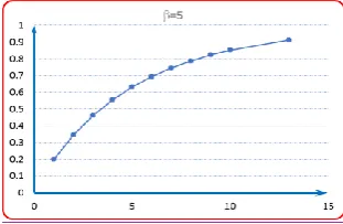
The Weibull shape parameter, β, is also known as the Weibull slope. This is because the value of β is equal to the slope of the line in a probability plot. Different value of the shape parameter can have marked effects on the behavior of the distribution in fact, some values of the shape parameter will cause the distribution equations to reduce to those of the of the other distribution. For example, when β= 1, the pdf of the three-parameter Weibull reduces to that of the two-parameter exponential distribution. R; P [6].
Looking at the same information on a Weibull probability plot, one can easily understand why the Weibull shape parameter is also known as the slope. Later we will show how the slope of the Weibull probability plot changes with β. So we show that the models represented by the figures all have the same α.
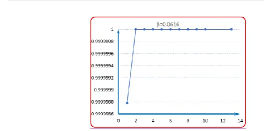
Another characteristic of the distribution where the value of β has a distinct effect is the failure rate. The following plot shows the effect of the value of β on the Weibull failure rate.
This is one of most important aspect of the effect of β on the Weibull distribution. As is indicated by the plot, Weibull distributions
with β have a failure rate, that decreases with time, also known as
infantile or early-life failures. Weibull distribution with β close to or equal to 1 have a fairly constant failure rate, indicative of useful life
or random failures. Weibull distribution with β have a failure rate
that increases with time, also as wear-out failures. Mixed Weibull
distribution with one subpopulation with β , one subpopulation
with and one subpopulation with would have a failure
rate plot that was identical to the bathtub curve.
b) Weibull scale parameter α
A change in the scale parameter α, has the same effect on the distribution as a change the abscissa scale. Increasing the value of α while holding β constant has the effect of stretching out the pdf. Since the area under a pdf curve is a constant value of one, the "peak" of the pdf curve will also decrease with the increase of α , as indicated in the
height decreases, while maintaining its shape and location.
2- If α is decreased, while β and µ are kept the same, the
distribution gets pushed in towards the left (i.e., towards its beginning or towards 0 or µ ), and its height increases.
3- α has the same unit as X , such as hours , mile, cycles,
actuations, etc. 8.5 Weibull plot
The fit of data to a Weibull distribution can be visually assessed using a Weibull plot [7]. The Weibull plot is a plot of the empirical
cumulative distribution function of data on special axes in a type
of Q Q plot the axes are versus . the reason for
this change of variables is the cumulative distribution function can be linearized:
there (3)
Which can be seen to be in the standard from of a straight line. Therefore, if the data came from a Weibull distribution then straight line is expected on a Weibull plot. There are various approaches to obtaining the empirical distribution function from data: one method is
to obtain the vertical coordinate for each point using where
i is the rank of the data point and n is the number of data point Wayne Nelson [8]
Linear regression can also be used to numerically asses' goodness of fit and estimate the parameters of the Weibull distribution. The gradient informs one directly about the shape parameter and the scale parameter α can also be inferred.
8.6 Weibull Reliability
simplicity. Note that in the rest of this section we will assume the most general form of the Weibull distribution, the three- parameter form. The appropriate substitutions to obtain the other form, such as the two-parameter form where µ=0, or the one-parameter form where β is a constant, can easily be made.
The Weibull reliability function is given by: (4)
The Weibull failure rate function is given by:
ℎ (5)
The Weibull mean life is given by: (6)
Where is gamma function The gamma function is defined as:
(7)
The equation for the median life for Weibull distribution is given by: +α (8)
9. Estimation of Weibull Distribution parameter's
9.1 Graphical procedure
actually represented the order statistics
If we let ⸴ ⸴ ⸴ then represent a
simple linear regression corresponding to:
(9)
Where is intercept of the linear equation we perform the estimation
of α and β using the following methods of estimation .
9.2 Maximum Likelihood Estimation(MLE)
The method of maximum likelihood estimation used for estimating parameters Cohen and Harter and Moore (1965).
Let be a random sample of size n drawn from a population
with probability density function is defined by (11)
The maximum likelihood of maximize L or equivalently ,
the logarithm of L when
(12)
for example, Mood et al (1974). Consider the Weibull pdf given in equation its likelihood function is given as:
(13)
Taking a natural logarithm of both sides yields:
(14)
And differentiating equation (14) partially w.r.t β and ⸴ in turn and equating to zero obtain the estimating equation as follows :
(15)
And (16)
From (16) we obtain an estimator of as
(17) And on substitution of (17) in (15) obtain
(18)
9.3 Least squares method (LSM)
The least squares method assume that there is a linear relationship between two variables assume a data set that constitute a pair
( were obtained and polled the
least square principle minimizes the vertical distance between the data points and straight line fitted to the data ⸴the best fitting line to
this data is the straight line : such that
(19)
To obtain the estimators of α⸴ and β we differentiate Q w.r.t α ⸴β. Equating to zero
Subsequently yields the following system of equation: (20)
(21)
Expanding and solving equation (20), (21) simultaneously, we have (22)
And
(23)
Where and are the unbiased estimators of the α and β
respectively.
9.4 Weibull Regression
Another approach to finding parameters for a Weibull distribution is based on linear regression first note that the cumulative distribution function of a Weibull distribution can be expressed as
And so
Taking the natural log of both sides of the equation yields the equation
Multiplying both sides of equation by -1 and taking the log again yields' the equation
Where
Thus if the sample has a Weibull distribution then we should be able to find the coefficient linear regression [9]
10- Goodness-of fit test
A goodness-of fit test is appropriate when one wishes to decide if an observed distribution of frequencies is incompatible with some preconceived or hypothesized distribution [10] by other the test procedures are intended to defect the existence of a significant difference between the observed (empirical) frequency of occurrence of an item and the theoretical(hypothesized) patter of occurrence of data here we assume that the Weibull distribution is a good fit to the given data set ; otherwise, this assumption is nullified.
A goodness- of fit test is
11. Application
In this section we apply to a data which is the time of breast cancer patients in moths we focus on analysis using Weibull distribution of two parameters model. The sample data obtained from ministry of health in Khartoum state in year 2016- 2017 and sample data in table (1) bellow.
Table 1. sample patient times pear month of breast cancer
2 2 10 3 2 9 6 10 6 1
3 13 8 4 4 4 4 8 5 10
4 5 4 6 1 4 4 6 6 8
6 2 4 6 4 6 2 4 5 6
6 4 4 6 10 8 5 4 6 4
5 1 6 4 8 2 13 6 4 9
6 10 8 4 6 4 5 8 4 4
4 8 2 5 4 6 2 5 2 4
4 6 4 5 4 6 4 2 5 6
2 4 6 13 7 5 1 3 13 8
5 4 6 5 6 6 10 3 5 5
13 9 5 2 8 4 8 6 2 2
5 6 6 4 5 5 6 6 4 4
2 8 4 1 2 13 4 5 1 6
Sources data: military medical hospital
We calculate from data the estimated value of , using the formula
parameter, whereas Xi represent times patient of breast cancer and Oi represent observed frequency looking in table ( 2) bellow
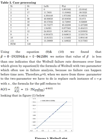
Table 2. Case processing
Xi Oi LnXi F(x) y
1 6 0 3.801582 -23.8342
2 17 11.7835 11.03802 -38.5525
3 4 4.394448 1.975392 -6.48534
4 36 49.90658 23.93856 -33.873
5 19 30.57932 12.72983 -6.02668
6 30 53.75277 20.22288 5.427269
7 1 1.94591 0.677563 0.484315
8 12 24.9533 8.166744 8.235932
9 3 6.591675 2.049615 2.535178
10 6 13.81551 4.113402 5.804146
≥11 6 15.38969 4.148622 9.317563
SUM 140
Using the equation (9)& (10) we found that
we notice that value of is less than one indicates that the Weibull failure rate decreases over lime which given by equation(5) the formula of Weibull with two parameter which often use in failure analysis, because no failure can happen before time zero. Therefore,µ=0, when we move from three- parameter to the two-parameter we have to do is replace each instance of with , the formula for the pdf reduces to:
looking that in figure (1) below
Figures 1: Weibull plot
(9), (22), (23) and the calculations in above table and the linear regression model represented with equation:
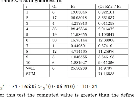
to check the hypotheses uses a goodness- of fit test to find the statistics using table (3) bellow
Table 3. test of goodness fit
i Oi Ei (Oi-Ei)2 / Ei
1 6 19.03046 8.922161
2 17 26.93018 3.661637
3 4 4.217913 0.011258
4 36 28.42864 2.016472
5 19 11.98655 4.103647
6 30 15.75144 12.88908
7 1 0.449501 0.67419
8 12 4.714465 11.25876
9 3 1.046555 3.646198
10 6 1.881927 9.011256
>=11 6 25.56238 14.9707
SUM 71.16535
Figure 2: effect of Weibull shape parameter on probability
Figure 3: effect of Weibull shape parameter on probability
Figure 4: effect of Weibull shape parameter on probability
Figure 6: effect of Weibull shape parameter on probability
12. CONCLUSION
In this paper find that results as follows:
1- The data of the breast cancer distributed with linear model
2- The linear regression can also be used to numerically assess goodness of fit to estimate the parameters of Weibull distribution
3- The failure rate decreases over time.
13.RECOMMENDATION
Based on the results the paper recommends the following:
1- Weibull recommended because it has flexibility to process
difference data
2- using linear model if other methods cannot be a good fit to
estimate model parameters.
REFERENCES
[1] Papoulis, Athanasios Papoulis; Pillai, S. Unnikrishna (2002).
Probability, Random Variables, and Stochastic Processes (4th ed).
Boston: McGraw-Hill. ISBN 0-07-366011-6
[2] Sharif, M.Nawaz; (1980), "The Weibull distribution as a general model for forecasting technological change".
[3] Rinne.H, (2008), "the Weibull distribution"
[4] Al-Fawzan. M (2000). "Methods for Estimating the Parameter of the Weibull Distribution" King Abduaaziz City for Science
[5] Nwbi.F.N, Ugomma.Ch.A, (2104),"Comparison of Methods for the Estimation of Weibull Distribution Parameters,
[6] Jiang, R.; Murthy, D.N.P (2011)." A study of Weibull shape parameter: Properties and significance". Reliability Engineering and system Safety. 96(12): 1619-26.
[7] Weibull Plot "
(http://www.itl.nist.gov/div898/handbook/eda/section3/welibplot.htm )www.itl.nist.gov.
[8] Wayne Nelson (2004) "Applied Life Data Analysis. Wiley-Blackwell ISBN0-471-64462-5
[9] Law less J.F (2003),"Statistical Models and Methods for Life Time Data" Edition, John Wiley and Sons, New York