genomic and behavioural evolution in the artificial ecosystem simulation EcoSim

(1)

University of Windsor University of Windsor

Scholarship at UWindsor

Electronic Theses and Dissertations Theses, Dissertations, and Major Papers

2014

genomic and behavioural evolution in the artificial ecosystem

simulation EcoSim

Marwa Fouad Khater University of Windsor

Follow this and additional works at: https://scholar.uwindsor.ca/etd

Recommended Citation Recommended Citation

Khater, Marwa Fouad, "genomic and behavioural evolution in the artificial ecosystem simulation EcoSim" (2014). Electronic Theses and Dissertations. 5204.

https://scholar.uwindsor.ca/etd/5204

This online database contains the full-text of PhD dissertations and Masters’ theses of University of Windsor students from 1954 forward. These documents are made available for personal study and research purposes only, in accordance with the Canadian Copyright Act and the Creative Commons license—CC BY-NC-ND (Attribution, Non-Commercial, No Derivative Works). Under this license, works must always be attributed to the copyright holder (original author), cannot be used for any commercial purposes, and may not be altered. Any other use would require the permission of the copyright holder. Students may inquire about withdrawing their dissertation and/or thesis from this database. For additional inquiries, please contact the repository administrator via email

(2)

Genomic and behavioural evolution in the

artificial ecosystem simulation EcoSim

by

Marwa Fouad Khater

A Dissertation

Submitted to the Faculty of Graduate Studies

through School of Computer Science

in Partial Fulfillment of the Requirements for

the Degree of Doctor of Philosophy at the

University of Windsor

Windsor, Ontario, Canada,

2014

(3)

Genomic and behavioural evolution in the artificial ecosystem simulation EcoSim

by

Marwa Khater

APPROVED BY

———————————–

Dr. G. Arhonditsis ,External Examiner

University of Toronto Scarborough

————————————

Dr. J. Ciborowski, External Reader

Department of Biological Sciences

————————————

Dr. Z. Kobti, Internal Reader

School of Computer Science

————————————

Dr. A. Ngom, Internal Reader

————————————

Dr. R. Gras, Advisor

————————————

(4)

Declaration of Co-Authorship

I hereby declare that this dissertation incorporates material that is result of

joint research, as follows:

This dissertation also incorporates the outcome of a joint research undertaken

in collaboration with Marwa Khater and Dorian Murariu under the supervision of

professor Robin Gras. The collaboration is covered in Chapter 7 of the dissertation

whenever a biological discussion is required. In all cases, the key ideas, primary

contributions, experimental designs, data analysis and interpretation, were

per-formed by the author, and the contribution of co-authors was primarily through

the provision of required background biological information.

I am aware of the University of Windsor Senate Policy on Authorship and I

certify that I have properly acknowledged the contribution of other researchers

to my dissertation, and have obtained written permission from the co-author to

include the above materials in my dissertation. I certify that, with the above

qualification, this dissertation, and the research to which it refers, is the product

of my own work.

Declaration of Previous Publication This dissertation includes five original

pa-pers that have been published/submitted for publication in peer reviewed

(5)

Thesis Chapter Publication title/ full citation Publication status

Chapter 5 M. Khater, E. Salehi, and R. Gras, Published

”The emergence of new genes in EcoSim

and its effect on fitness,”

in Simulated Evolution and

Learning. Springer, 2012, pp. 52-61.

Chapter 5 M. Khater and R. Gras, Published

Chapter 6 ”Adaptation and genomic

evolution in EcoSim,”

From Animals to Animats

12, pp. 219-229, 2012.

Chapter 6 M. Khater, E. Salehi, and R. Gras, Published

”Correlation between genetic diversity

and fitness in a predator-prey

ecosystem simulation,”

in AI 2011: Advances in

Artificial Intelligence. Springer,

2011, pp. 422-431.

Chapter 7 M. Khater, D. Murariu, and R. Gras. Published

”Contemporary evolution and

genetic change of prey as

a response to predator removal.”

Ecological Informatics,

22:13-22, 2014.

Chapter 7 M. Khater, D. Murariu, and R. Gras. Submitted

”Predation risk tradeoffs in prey:

effects on energy

(6)

Abstract

Artificial life evolutionary systems facilitate addressing lots of fundamental

questions in evolutionary genetics. Behavioral adaptation requires long term

evo-lution with continuous emergence of new traits, governed by natural selection.

We model organism’s genomes coding for their behavioral model and represented

by fuzzy cognitive maps (FCM), in an individual-based evolutionary ecosystem

simulation (EcoSim). The emergent of new traits (genes) in EcoSim is examined

by studying their effect on individual’s fitness and well being. We examine how

the new traits are used to predict the value of fitness using machine learning

tech-niques. A comparison between the genomic evolution of EcoSim and a neutral

model (a randomized version of EcoSim) is examined focusing on their respective

genomic diversity. In order to further emphasize the importance of genetic

diver-sity to adaptation and thus the well being of individuals, we were encouraged to

study the effect that genetic diversity has on fitness. EcoSim gives us the chance

to study the relation between species genetic diversity and average species fitness

without the limits in environmental conditions and time scales found in biological

studies, but in highly variable environments and across evolutionary time.

The ecological effects of predator removal and its consequence on prey

behav-ior have been investigated widely. We investigated the effects of predation risk

on prey energy allocation and fitness. Here the role of predator removal on the

contemporary evolution of prey traits such as movement, reproduction and

for-aging was evaluated. Our study clearly shows that predation risk alone induces

behavioural changes in prey which drastically affect population and community

dynamics, A classification algorithm was used to demonstrate the difference

be-tween genomes belonging to prey co-evolving with predators and prey evolving

in the absence of predation pressure. We argue that predator introductions to

naive prey might be destabilizing if prey have evolved and adapted to the absence

of predators. Our results suggest that both predator introduction and predator

removal from an ecosystem have widespread effects on the survival and evolution

of prey by altering their genomes and behaviour, even after relatively short time

(7)

Acknowledgments

Foremost, I would like to express my sincere gratitude to my supervisor Dr. Robin

Gras for the continuous support of my PhD study and research, for his patience,

motivation, enthusiasm, and immense knowledge. His guidance helped me in all

the time of research and writing of this thesis. He has always allocated time for me

and was constantly giving me advice. I could not have imagined having a better

supervisor and mentor for my PhD study. I would like to thank my committee

members Dr. George Arhonditsis, Dr. Jan Ciborowski, Dr. Ziad Kobti and Dr.

Alioune Ngom for accepting to allocate part of their valuable time to evaluate my

research.

I would like to extend my gratitude towards Dorian Murariu, my research

part-ner and biology cohort, who meticulously helped me in collecting all the required

biological information needed for this research. His valuable insight and comments

added depth to this thesis. I also like to thank all my team mates and other lab

members specially Abbas Golestani, Morteza Mashayekhi and Yasaman Farahani

who throughout this journey became dear friends. They gave me their comments

and technical help when needed.

Special thanks must go to my husband and life-partner Rami Salem. He

pro-vided unconditional love, support and encouragement through both the highs and

lows of my time in graduate school.

Finally, I like to thank and dedicate this thesis to my mother Dr. Sanaa Alassar

who has always believed in me and constantly pushed me forward. I derive my

strength through her.

This work was made possible by the facilities of Shared Hierarchical

Aca-demic Research Computing Network (SHARCNET: www.sharcnet.ca) and

(8)

List of Tables

3.1 Several physical and life history characteristics of individuals from

10 independent runs. . . 20

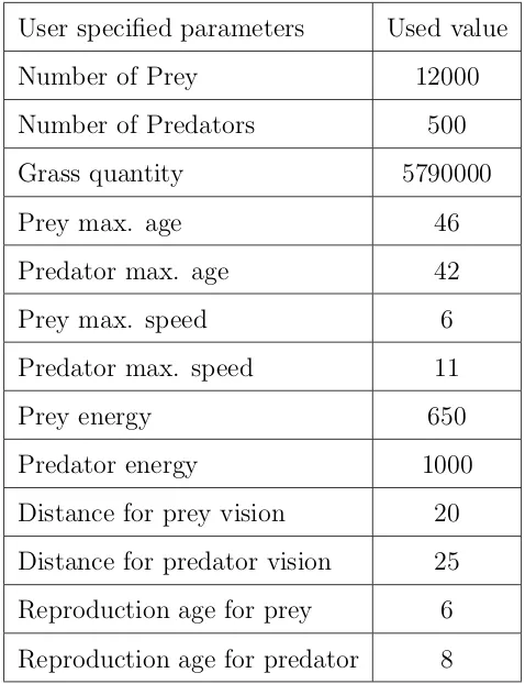
3.2 Values for user specified parameters. . . 34

5.1 Percentage of low fitness (LOW), high fitness (HIGH), and very

high fitness (VHIGH) prey instances for 4 different runs. . . 52

5.2 Accuracy for training and validating with the Random Forest

clas-sifier on four runs of the simulation. . . 53

5.3 Accuracy percentages for training and validating with JRip after

CMSS-EDA and CfsSubsetEval feature selection, for four runs of

the simulation. . . 54

6.1 Percentage of high positive (HIGHP), high negative (HIGHN), weak

correlation (WEAK CORR) between fitness and genetic diversity

for window of 400 and shift of±25 for five different runs. . . 66

6.2 Accuracy percentages for training and validating with the C4.5

clas-sifier for 5 runs of the simulation. . . 67

6.3 Accuracy percentages for training and validating with the RF

clas-sifier for 5 runs of the simulation. . . 68

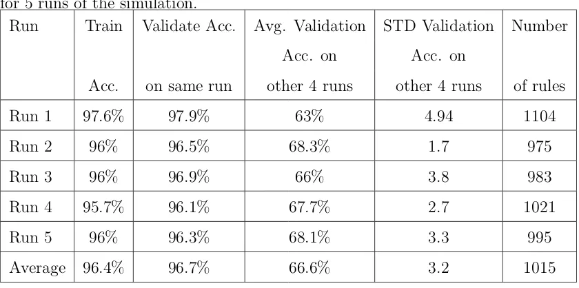
6.4 JRip rule learner accuracies and number of produced rules for five

(13)

7.1 Average energies (with std between brackets) consumed by prey

while engaging in each type of action, expressed as a percent of

their average energy budgets. (Note: since these are average values

over the entire duration of the runs they do not add up to 1). Eating

represents net energy gained from eating, including the energy spent

on the eating action itself. Due to computational limitations we

present here the average energy consumed for each action for four

runs of case A and B prey only. *Includes all successful and failed

actions. . . 85

7.2 Demographic characteristics as a percent (%) of population for case

A and B runs. Standard deviations in brackets. *Includes successful

and failed actions. **Death rate includes all causes of death (being

eaten by predators (for case A prey only), energy depletion, and

old age). . . 87

7.3 Average frequency of movement actions of all prey as a percent (%)

of the total population of prey, for case A and B prey except for

Speed which is expressed as number of cells. Standard deviations in

brackets (std).*Includes all successful and failed attempts for each

action. . . 90

7.4 Accuracy for training the classifier using 10 fold cross validation,

accuracy of validating the classifier using the validation set, and the

number of rules produced from the model . . . 95

(14)

List of Figures

3.1 The overview and scheduling of every time step. . . 23

3.2 Initial FCM prey map including concepts and edges. The width of

each edge represents the influence value of a concept on another.

Color of an edge shows inhibitory (red) or excitatory (blue) effects. 25

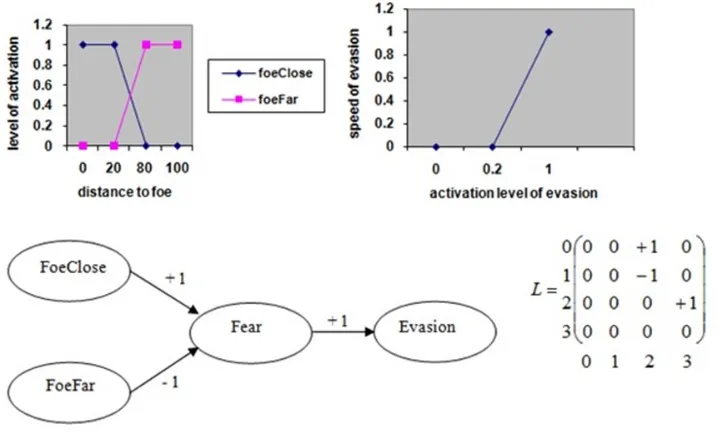
3.3 An FCM for detection of foe (predator) and decision to evade with

its corresponding matrix (0 for ’Foe close’, 1 for ’Foe far’, 2 for

’Fear’ and 3 for ’Evasion’) and the fuzzification and defuzzification

functions. . . 25

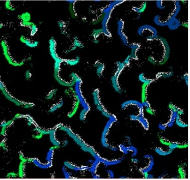
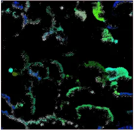
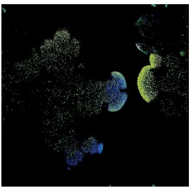
3.4 The snapshot of the virtual world in one specific time step, white

color represents predator species and the other colors show different

prey species. . . 27

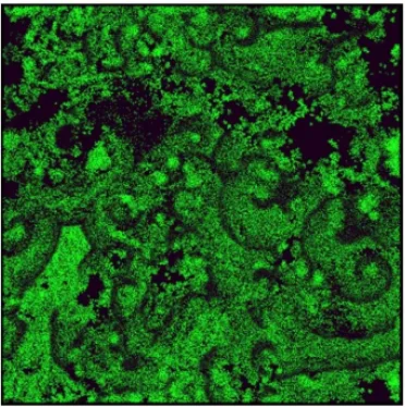
3.5 The snapshot of the virtual world for a specific time step of the

simulation which demonstrates the pattern of grass in the world. . . 28

3.6 FCM for detection of foe (predator) - difference between perception

and sensation. . . 31

3.7 Breeding algorithm. . . 36

3.8 Snap shot of the Neutral shadow world with predator and prey

spatial distribution . . . 38

5.1 Global Entropy for 10 different runs of the simulation. Top 5 curves

(15)

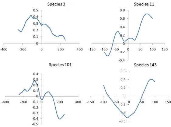
6.1 Different prey species correlation values between entropy and

fit-ness. x-axis represents the different time shifts. Y-axis represents

the correlation values. . . 61

7.1 Snapshot of the world in one of the case A runs at time step 5000.

The numbers of prey and predator individuals are 198554 and 27903

respectively. The colored spirals show different prey species and the

white represents predators. . . 76

7.2 Snapshot of the world in one of the case B runs at time step 5000

showing 34254 prey individuals. . . 77

7.3 Snapshot of the world in one of case C runs. Figure on right

rep-resents the world at time step 15000 showing 233784 prey and the

figure on left at time step 15060 where prey increased to 1040856. . 77

7.4 Total prey population. Blue line represents case A (high-risk prey),

red line represents case B (low-risk prey), and green line represents

case C where predators and prey co-evolve till 15,000 time steps,

and then prey evolve alone. . . 79

7.5 The average amount of grass in the world. Blue line represents case

A (high-risk prey), red line represents case B (low-risk prey), and

green line represents case C where predators and prey co-evolve till

15,000 time steps, and then prey evolve alone. . . 79

7.6 The average prey fitness. Blue line represents case A (high-risk

prey), red line represents case B (low-risk prey), and green line

represents case C where predators and prey co-evolve till 15,000

time steps, and then prey evolve alone. . . 80

7.7 The average prey populations choosing reproduction action,

includ-ing all successful and failed attempts. Blue line represents case A

(high-risk prey), red line represents case B (low-risk prey), and

(16)

7.8 The average prey birth ratio to population. Blue line represents

case A (high-risk prey), red line represents case B (low-risk prey),

and green line represents case C where predators and prey co-evolve

till 15,000 time steps, and then prey evolve alone. . . 81

7.9 Grass density is the total units of grass divided by the number of

prey population in the world. Blue line represents case A

(high-risk prey), red line represents case B (low-(high-risk prey), and green line

time steps, and then prey evolve alone . . . 83

7.10 The average prey foraging ratio to population. Blue line represents

case A (high-risk prey), red line represents case B (low-risk prey),

and green line represents case C where predators and prey co-evolve

till 15,000 time steps, and then prey evolve alone. . . 84

7.11 Percentage of maximum allowed transmitted energy to offspring at

birth. Blue line represents case A (high-risk prey), red line

repre-sents case B (low-risk prey), and green line reprerepre-sents case C where

predators and prey co-evolve till 15,000 time steps, and then prey

evolve alone. . . 87

7.12 The proportion of the total prey population runs that chose a

move-ment action (escape, foraging, socialize or explore) at each time

step. Blue line represents case A (high-risk prey), red line

repre-sents case B (low-risk prey), and green line reprerepre-sents case C where

predators and prey co-evolve till 15,000 time steps, and then prey

evolve alone. Total movement is the sum of all four of these actions,

and includes all successful and failed foraging and socialization

ac-tions. . . 89

7.13 The proportion of all movement actions that high (case A) and

low(case B) risk prey runs spent. The bars show a behavioural

tradeoff between time spent foraging and time spent responding to

(17)

7.14 The average prey speed. Blue line represents case A (high-risk

prey), red line represents case B (low-risk prey), and green line

time steps, and then prey evolve alone. . . 91

7.15 The average prey genetic distance from initial FCM map. Blue line

represents case A (high-risk prey), red line represents case B

(low-risk prey), and green line represents case C where predators and

prey co-evolve till 15,000 time steps, and then prey evolve alone. . 92

7.16 The average prey genetic diversity (measured by entropy). Blue

line represents case A (high-risk prey), red line represents case B

(low-risk prey), and green line represents case C where predators

and prey co-evolve till 15,000 time steps, and then prey evolve alone. 93

7.17 The average number of prey species. Blue line represents case A

(high-risk prey), red line represents case B (low-risk prey), and

15,000 time steps, and then prey evolve alone. . . 93

7.18 Distribution of genes appearing in the JRip classifier. . . 100

7.19 Snapshot of the world in one of the case D runs (predators are

in-troduced to naive prey) at time step 5000. Preys show more spatial

dispersal and white patches represent predators. In the first figure

the numbers of prey and predator individuals are 31502 and 1008

respectively. In the second figure at time step 5030 prey decreased

to 9301 and predators were 1502. At time step 5112 prey decreased

(18)

Chapter 1 Introduction

1.1 Motivation

Darwin (1859) conceived the mechanism that could account for the adaptation

and the diversity observed in nature. Darwin’s principle of natural selection rests

on a number of propositions [1]:

• The individuals of a population are not identical but vary in certain traits.

• This variation, at least partly, is heritable. Therefore, an individual shares some of these traits with its ancestors.

• Every population could potentially populate the whole world if each indi-vidual of that population realized its full reproductive potential. In reality,

few (if any) individuals do, and many individuals die without reproducing

at all.

• Individuals vary in their number of descendants (not only the number of children they produce, but the number of children that survive, and the

offspring they leave and so forth).

• The number of an individual’s descendants depends critically (but not

(19)

Populations with these characteristics, over generations, become more adapted

to their environment. With time and changing circumstances, different

adapta-tions may become advantageous. Gradually, this mechanism gives rise to different

life forms. Artificial Life (Alife) is concerned with the study of the processes and

mechanisms underlying life by recreating life-like phenomena in software,

hard-ware, and biochemicals [2]. The term ’artificial life’ was coined by Langton who

described Alife as ”a field of study devoted to understanding life by attempting to

abstract the fundamental dynamical principles underlying biological phenomena,

and recreating these dynamics in other physical media-such as computers-making

them accessible to new kinds of experimental manipulation and testing” [3].

An ecosystem is the complex system described by the organisms, the

environ-ment, and their physical, chemical and biological interrelationships in a given area.

Ecosystem health is determined through measurable characteristics. Ecosystem

health is determined through measurable characteristics. A healthy ecosystem is

defined as being ‘stable and sustainable’; maintaining its organization and

auton-omy over time and its resilience to stress [4]. So a healthy ecosystem is sustainable;

that is, it has the ability to maintain its structure (organization) and function

(vigor) over time in the face of external stress (resilience). A method to quantify

these attributes (vigor, organization, and resilience) should be taken into

consid-eration when modeling an ecosystem. Stability, population density, biodiversity

and how energy flows through trophic levels are some measurable characteristics

in evolutionary ecological models.

The metaphor of an evolving ecosystem was chosen for this study of

artifi-cial agent evolution because the evolutionary dynamics result from the modeling

of individual agents and their relations to the conditions and resources, in

com-bination with their diverse interactions with other agents in their environment.

Together, these factors make up the artificial ecosystem. This view of an evolving

system, where natural selection is an emergent system property, stands in contrast

to traditional evolutionary algorithms where evolution is the direct result of an

(20)

1.2 Objective

Like in many disciplines; simulation modeling played a great role in studying

evo-lutionary processes. Many ecological studies that require data of hundreds of years

can be obtained by simulation modeling that produces results in a matter of a few

hours or days depending on the computational cost of each system. Darwinian

evolution governed by natural selection is modeled in EcoSim (an individual based

ecosystem simulation). Our main challenge concerns the ability to understand the

evolutionary machinery and evolved behaviour in the system. This problem is

of particular importance in systems based on natural selection. The lack of an

explicit objective (predefined fitness) function makes spotting and understanding

the evolved behaviour of individuals a challenging task. Therefore, there must be

some other way to identify and understand qualitatively novel behaviour when

it emerges. The objective of the work was to capture the correlation between

different emerging behaviours arising in EcoSim in order to gain deeper

under-standing of the model and thus natural ecosystems. Here came the integration of

machine learning techniques as an analytical step for analyzing the vast amount

of information produced by the simulation. The main aim of this work is to study

the genomic evolution and emerging behaviours arising in EcoSim. Validating the

evolutionary machinery in EcoSim by studying the evolution of possible new genes

and behaviours was the first main focus. The validation step was achieved through

examining how the new possible genes are capable of predicting the fitness of prey

individuals and through a comparison between the genomic evolution of EcoSim

and its neutral model. EcoSim is a platform that allowed the study of different

ecological theories such as the relationship between species genetic diversity and

fitness. The success to map this study in EcoSim acted as a validation step of the

model and also a contribution to gain more insight about the correlation between

genetic diversity and fitness.

The complexity of behavioural interactions in predator-prey systems has

re-cently begun to capture trait-effects, or non-lethal effects, of predators on prey

via induced behavioural changes. Non-lethal predation effects play crucial roles in

(21)

foraging, movement, and reproductive behaviours of prey. Prey exhibit tradeoffs

in behaviours while minimizing predation risk (see Chapter 7 for details). EcoSim

allows complex intra- and inter-specific interactions between individual evolving

behavioural models called prey, as well as complex predator-prey dynamics and

coevolution in a tri-trophic and spatially heterogeneous world. Another part of

the study involved investigating the effects of predation risk on prey energy

allo-cation and fitness. The semantics of the system allows comprehensive analysis of

new genes and behaviours as they arise through a Darwinian evolutionary process.

We asked the following questions about prey in EcoSim: are there trait-mediated

effects on prey in the form of predation risk-foraging tradeoffs? How does the

tradeoff affect the energy of prey and allocation of energy to reproduction? How

do their reproductive strategies change in response to predation? What are the

effects of predation risk on the prey population? Does the predation pressure

af-fect prey’s genomic evolution? How does prey evolve in the absence of predation

pressure? What is the effect of introducing predators to nave prey?

1.3 Contributions of the thesis

• First, the evolutionary machinery in EcoSim was studied by examining the emergence of new genes and their effect on fitness. Random Forest was used

to build a classifier that was able to predict the values of fitness based on

the values of new developed genes. This is considered to be a validation

step to ensure the validity of the behavior model and its ability to cope with

changes in the environment. A feature selection step is then presented along

with rule learning. These rules allow us to discover the most important

features that increase fitness, and help us to understand the semantics of

the behavior model.

• It has been shown how genetic evolution and diversity governs the

adapta-tion process. We study how EcoSim’s individuals adapt to their changing

environment by comparing their behavior with a neutral model - a partially

(22)

• Shannon entropy, which is a measure of unpredictability and disorder com-ing from Information theory, is used as a measure of genetic diversity. We

present the difference in entropy between EcoSim and the neutral model

to emphasize the adaptive characteristics of EcoSim. Furthermore, we

in-vestigate the relationship between genetic diversity and species fitness and

present the correlations found between these two measures in EcoSim. Very

high correlation both negative and positive between entropy and fitness was

detected. In order to validate the correlation results and further

under-stand the reasons behind these results machine learning classifiers were used

to predict the correlation class variable based on training and testing sets.

High accuracy for classification was seen which proves the interest of the

used genetic diversity measure and its correlation with fitness. In addition,

feature selection step was used to find the best features affecting the

corre-lation values. These extracted features such as popucorre-lation size and spatial

dispersal are similar to the factors affecting the relation between genetic

di-versity and fitness in community ecology. Rules were extracted and further

investigated which adds more semantics to the reasons behind correlation

between genetic diversity and fitness.

• EcoSim models predators and prey with a great deal of detail to their char-acteristics and interactions. In this study the effect of predator removal

on prey’s behaviour (foraging, movement and reproduction), genetic change

and their capability to coevolve when predators are reintroduced in EcoSim

is investigated. In addition, prey are allowed to evolve along two distinct

evolutionary paths in the simulation, by either coevolving with predators

or evolving in their absence. Results revealed that prey energy budgets,

life history traits, allocation of energy to movements and fitness-related

ac-tions differed greatly between prey subjected to low-predation risk versus

high-predation risk. High-predation risk suppressed prey foraging activity,

increased movement, and decreased reproduction relative to low-risk. We

used a classification algorithm to show that distinct genomes, corresponding

to distinct behavioural adaptations in these prey populations, had evolved

(23)

that prey alter their behaviour according to the level of predation risk. In

particular, prey reduce their foraging effort when predation risk is high and

instead invest more resources in antipredator behaviours. In addition, these

risk-aversive behaviours negatively influence prey fitness as they reduce

en-ergy that can be allocated to reproduction. The introduction of predators to

naive prey was also studied and monitored predator-prey dynamics, along

with the stability of the system after this change. We show that the prey

that are left to evolve for a long time without predators developed survival

strategies and adaptive behaviors that were coded in their genomes, and this

caused instability in the system when predators were later introduced.

1.4 Outline of thesis

• Chapter 2 reviews existing literature on evolutionary systems and the use of

IBM in ecology, with a particular focus on ALife evolutionary simulations.

• Chapter 3 gives an overview of, the model used in this study, EcoSim which is

a predator-prey ecosystem simulation that is capable of exhibiting long-term

adaptive evolution of agent behaviour.

• Chapter 4 presents the background of the data analysis approaches used in the rest of the thesis including machine learning techniques, the deployment

of entropy as a measure of genetic diversity and fitness calculation.

• Chapter 5 presents the details of studying the emergent of new genes in EcoSim and its effect on average species fitness. The comparison between

genetic diversity in EcoSim and its neutral model, which is affected by

con-tinuous adaptation of the individuals to their dynamic environment, is also

reviewed.

• The study of genetic diversity and its correlation with fitness is presented in Chapter 6 along with the classification and rule extraction step used to add

(24)

(25)

Chapter 2 Background and Literature

Review

2.1 Artificial life

Artificial Life, or ALife, is the research field that tries to describe and study

nat-ural life by creating artificial systems that possess some of the properties of life.

The notion Artificial Life was first presented by Langton who described it by

”understanding life by attempting to abstract the fundamental dynamical

prin-ciples underlying biological phenomena, and recreating these dynamics in other

physical media, such as computers, making them accessible to new kinds of

ex-perimental manipulation and testing.” [3]. Latter on Bedaue noted Artificial Life

is concerned with the study of the processes and mechanisms underlying life by

recreating life-like phenomena in software, hardware, and biochemicals [2]. There

are three methods to model ALife; ’soft’ that uses software simulations, ’hard’

which involves hardware implementation mainly in robotics and ’wet’ which

in-volves biochemistry. The first known formal model was designed by John von

Neumann creating a self-reproducing, computational universal cellular automata

[5]. He formalized the idea of cellular automata in order to create a theoretical

model for a self-reproducing machine. He was mainly concerned with studying

the evolution of complex adaptive structures motivated by the understanding of

(26)

informa-tion theory aiming to understand living systems was done by Wiener [6]. Due to

the increase use of computer simulations, Alife has overlapped and associated with

other areas in artificial intelligence such as computational intelligence, which is a

nature-inspired computational methodology that addresses real world

optimiza-tion problems. Although computaoptimiza-tional intelligence and Alife overlap in many

aspects and share similar methodology, there is a difference in their modeling

strategies. Alife is mainly concerned with gaining knowledge about living systems

using computational bottom-up complex systems. On the other hand,

computa-tional intelligence is motivated by the inverse, mainly using the knowledge about

living system to construct a top down centralized complex system. Whereas,

computational intelligence research is essentially analytic, breaking down complex

systems into basic components, ALife synthetic approach attempts to construct

complex systems from elemental units. The synthetic approach is based on two

concepts, emergence and adaptation.

Complex adaptive systems exhibit emergence where the behavior of the whole

is more complex than the behavior of the parts [7]. Emergence is one of the

char-acteristics of a complex system where new and coherent structures, patterns in a

complex system are derived due to interactions between the elements of the system

over time [8]. The characteristics of emergence were provided by Holland[7]. (a)

Emergence happens in systems which compose of different interactive units that

follow simple rules. (b) The interactions between the parts are nonlinear so the

overall behavior cannot be predicted by summing the behaviors of the isolated

parts. (c) The system functions change with the change of context which makes it

difficult to predict emergent behavior. (d)The general trend of system complexity

increases with increasing number of interactions. [9] defines emergence as ”the

origin of qualitatively new structures and functions which were not reducible to

those already in exist”. He classified the emergent phenomena into three different

classes; computational emergence which is derived from the cellular automaton

example and the mathematical theory of chaos, thermodynamic emergence which

is the physicists way to emergent phenomena, and emergence relative to a model

which deals with situations where observers need to change their model in order

(27)

emer-gence relative to a model category. Evolutionary emeremer-gence is an essential feature

in Alife as [10] noted ”The essential features of computer-based Artificial Life

models are: . . . There are no rules in the system that dictates global behavior.

Any behavior at levels higher than the individual programs is therefore emergent.

There are two types of selection that might bring such emergence. [11] referred

to these as ”extrinsic adaptation where evolution is governed by a specified

fit-ness function, and intrinsic adaptation, where evolution occurs automatically as a

result of dynamics of a system cause by the evolution of many interacting

subsys-tems”. When aiming to model a more open-ended evolution Alife system, intrinsic

adaptation should be diploid.

Artificial evolving systems with pre-defined fitness functions, or fitness

land-scapes, have been well studied. GAs are biologically inspired search procedures

initially developed by Holland [12] [13] [14] in the early 1960s. GAs evolve an

initial random population of genomes (codings for solutions to the problem in

hand) by selecting which individuals reproduced and which will be replaced. This

is done by evaluating each solution’s fitness function relevant to the problem and

favouring the fitter solutions. A basic shortcoming of genetic algorithms and

evo-lutionary algorithms in general is their tendency to converge. They treat evolution

as an optimizer, as they reach local or global optima and eventually converge

to-wards them. When the goal becomes building a system where autonomous agents

are able to evolve and adapt in a more open-ended evolutionary dynamics,

spec-ifying in advance all the possible behaviours by optimizing an objective function

is not desirable. When targeting unbounded evolution and emergence of new

adaptive behavior, evolutionary algorithms (using extrinsic adaptation) should be

rejected and rather a model based on natural selection (intrinsic adaptation) is

more suitable. Furthermore, most existing theoretical modeling approaches rely

on the genetic algorithms (GAs) model concept. These systems are

optimiza-tion processes, meaning that the fate of the system is directly determined by its

(28)

2.2 IBM

Soft Alife uses individual-based modeling (IBM) which is a bottom-up approach

to simulating the interactions among individuals or groups of individuals in an

attempt to create complex phenomena. IBM differs from classical equation based

models (EBMs) which are typically built up from set of interrelated differential

equations. Unlike EBMs, IBM consists of interacting adaptive entities which are

able to capture emergent behavior and provide a greater level of useful details.

The ease of modeling renders IBM as being more flexible than EBM. IBM has

been used on non-computing related scientific domains such as ecological sciences

(surveyed by [15]) and social sciences (surveyed by [16]).

The benefits of IBM over other modeling techniques can be captured in several

points [8]: (i) agent-based models are a natural way to describe systems comprised

of interacting entities; (ii) agent-based models are flexible; (iii) agent-based

mod-els capture emergent phenomena; and (iv) agent-based modmod-els provide access to a

greater level of useful detail. In particular, modeling interactions between entities

can be much easier in agent-based systems than in EBMs, even when one is

com-fortable with the concepts of partial differential equations. It is usually easy to

increase the size of a simulation, adding new agents to see if interesting effects are

swamped by agent numbers, or taking agents away if interesting detail is obscured.

It is also possible to look at the results of simulations at different levels of detail

at the level of a single agent, at the level of some specific group of agents, or at

the level of all agents together. All these things are harder to manage in EBMs.

In addition to their inherent naturalness and flexibility, agent-based simulations

allow one to identify emergent phenomena. Emergent phenomena result from the

actions and interactions of individual agents, but are not directly controlled by

the individuals.

For the past decade there has been an enormous growth of use of IBM

ad-dressing different questions in ecology and evolutionary biology. Whereas classical

approaches to modeling ecology often ignore individual behaviour and instead uses

state- variable model that controls birth and death rates, IBM aim to ”treat

(29)

more realistic simulation. The use of IBM in ecology and evolution has been

re-viewed by Grimm in 1999 and Lomnicki 1999 [18]. DeAngelis and Mooij presented

another review study which focused on how the IBM field developed [15].

DeAn-gelis categorized the different directions along which to study individual variation

in IBM into five different directions ”(a) spatial variability, local interactions and

movement; (b) life cycle and ontogenetic development; (c) phenotypic variability,

plasticity and behavior; (d) differences in experience and learning; and (e) genetic

variability and evolution.” He also grouped the IBM systems into seven major

study groups; movement through space, formation of patterns among

individu-als, foraging and population dynamics, species interactions, local competition and

community dynamics, evolutionary processes, management related processes. A

book by Grimm and Railsback (2005) [19] provides a set of guidelines for building,

testing, and analyzing individual-based models, updated in [20]. IBM has been

used in many areas in ecology including forest ecology (e.g. [21]), fisheries and

marine life (e.g. [22]), conservation biology and spatial heterogeneity (e.g. [23]).

Many ecological IBM systems were not designed to be general platforms that could

capture different aspects in ecology and evolution but rather these models answer

specific question in their narrow domain. More group of evolutionary IBMs that

were designed as platforms studying evolutionary behavior, emergence, adaptation

and complexity are mention below.

2.2.1 Tierra

While evolutionary computation has been studied since the 1960’s, the subfield of

digital evolution is much younger. The first experiments with populations of self

replicating computer programs were performed in 1990 in a system called

Core-world [24], and later improved upon in Tierra [25]. Tom Ray’s Tierra model is

the first widely known digital evolutionary ecosystem consisting of self-replicating

computer programs based on natural selection. Competition in Tierra results from

finite CPU-time and memory space. Tierra is based on a virtual operating

sys-tem, complete with its own, relatively robust and simple (but universal) machine

(30)

empty memory space with a hand-written self-replicator program. This replicator

then produces a copy of itself which is instantiated as an independent process. A

small amount of stochastic behaviour is implemented for program execution, the

copy process, and programs are also subject to point mutations. These

mecha-nisms are responsible for introducing variety into the populations. If the modified

programs retain their ability to replicate, and the modifications alter their

prob-ability of reproduction, Darwinian evolution can occur. A number of interesting

results have been obtained from such evolutionary runs. For example, ’parasites’

have appeared-short pieces of code which run another program’s copying

proce-dure in order to copy themselves. Hyper-parasites (parasites of parasites) have

also been observed, along with a number of other interesting ecological

phenom-ena. Ray demonstrated that it is possible to build an operating system in which

self-replicating computer code can evolve. On the other hand, after a certain

amount of time, Tierra fails to produce any new programs but only change in the

number of existing ones.

Rey sparked a number of follow-up systems based on Tierra. Cosmos a

Tierra-like system configured in a 2 dimensional toroidal Tierra-like grid environment was used

to study the role of contingency in evolution [26]. Furthermore, in Amoeba [27]

the language of the digital organism along with its self replicating code is also

subject to evolution. The Amoeba system, developed by Pargellis, showed the

possibility of spontaneous emergence of a self-replicating program.

2.2.2 Avida

Development of AVIDA (a Tierra like system) [28] [29], in which self-replicating

digital organisms consists of a circular list of instructions (its genome) and a

vir-tual CPU evolve. In Avida, each organism lives in its own address space, unlike

Tierra’s shared address space. This enhancement increased the power of digital

evolution as an experimental tool. AVIDA environment comprises a number of

cells, each cell can contain at most one organism, and the size of an AVIDA

pop-ulation is bounded by the number of cells in the environment. Organisms are

(31)

an offspring. When an organism replicates, a cell to contain the offspring is

se-lected from the environment and its inhabitant organism is replaced (killed and

overwritten). Since digital organisms are self-replicating and compete for space, a

higher merit (all else being equal) results in an organism that replicates more

fre-quently, spreading throughout and eventually dominating the population. Hence,

AVIDA satisfies the three conditions necessary for evolution to occur: replication,

variation (mutation), and differential fitness (competition). Individuals in Avida

do not move and in order to measure the complexity they use a fixed environment

which is rarely seen in nature. This means that the system is only adapting to

a preexisting environmental complexity. The processes derived from Avida and

Tierra are optimization processes, similar to evolutionary algorithms, for which

it has been proved that it converge toward a maximum, either local or global.

Finally, as with Tierra, the complexity growth in Avida always reaches an upper

bound and stops. These results with Avida do not capture the kind of continual

growth in qualitative complexity or long term incremental evolution that we can

observe in the biosphere. Hence, Avida and Tierra do not represent an open-ended

evolution which has been defined in various ways. Nehaniv, for example, defines

open-ended evolution as an unbounded increase in complexity [30]. In [31] Taylor

noted about Tierra and Tierra like systems ”most of these systems are only capable

of producing innovations of the ’more-of-the-same’ variety (e.g. more optimized

code), rather than anything fundamentally new.”

Avida was used to study numerous aspects of evolution [32]; issues of

complex-ity in evolution [33] [34]. Furthermore, they investigated the emergence of complex

behavior [35]. They showed that complex features do not appear suddenly but

only evolve when simpler traits exist which served as a foundation upon which

these complex features were built. In a recent study they showed how runaway

sexual selection leads to good genes and how they should be viewed as interacting

mechanisms that reinforce one another [36]. Evolving digital ecological networks

(32)

2.2.3 Echo

A significant advance in evolutionary IBM was presented by J. Holland in Echo

[37], a generic ecosystem in which agents evolve in a resource limited environment.

The world is made up of a square toroid lattice of sites which has different kinds

of evolving resources encoded by a letter. Agents interact with their environment

and are able to move from one site to another. They gain energy by eating and

spend it on their actions such as fighting, trading and mating. Reproduction

in Echo happens when an agent has replicated itself with a possible mutation

when it has gained enough resources to copy its genome asexually or by sexual

mating. Selection is based on the interacting agents rather than by a predefined

fitness function. Emerging phenomena arise such as formation of communities and

trading networks. Echo was used to study the modeling of food web complexity

[38]. Echo was intended to be a general model of intrinsic adaptive system rather

than modeling and answering specific questions in evolutionary biology. Due to

the high abstraction level of the Echo model, the degree of fidelity to real systems

is uncertain.

2.2.4 Polyworld

In PolyWorld [39], more advanced haploid agents, each controlled by an artificial

neural network, with a set of primitive behaviors and learning strategies,

popu-late a continuous environment containing number of energy sources (’food’) upon

which they rely on for survivor. Possible actions for agents include eat, mate, fight,

move, focus and light (for vision). Agents evolve under the influence of natural

selection and die when their energy is fully depleted or loose fight with another

agent. An agent’s genome specifies characteristics of its physiology and neural

ar-chitecture which is adapted during its life through Hebbian learning. Yaeger was

able to report the emergence of new population behavior such as fleeing, grazing,

following and flocking. Polyworld was used to study how evolution guides

com-plexity [40] and the passive and driven trends in the evolution of comcom-plexity [41].

Genetic clustering for the identification of species was presented was also presented

(33)

Polyworld, makes it difficult to reason and link together different aspects of the

model. Another criticism of PolyWorld, in the context of perpetual evolutionary

emergence, is that learning appears to be overwhelmingly responsible for the

re-sults. This integrated learning process adds to the computational complexity of

the model. Furthermore, the high complexity of the neural networks agents limits

their number making it difficult to study large ecosystem phenomena’s. Geb [43]

[44] is another similar artificial neural network system considered to be simpler

than Polyworld as it is not trying to mimic the real world as Polyworld do. Agents

which are controlled by a neural network each populate a gridded arena and

com-pete for space with no notion of energy. There is no learning process as agents do

not change during their lifetime and thus results prove it to be suited to long-term

incremental artificial evolution. Geb was proven to be the first autonomous

arti-ficial system to pass the Bedau and Packard’s evolutionary test [45]. According

to Bedau statistics, evolutionary dynamics in Gep was proven to be unbounded

[46] and thus based on intrinsic evlution. Bedau et al [45] developed a statistical

measure for testing unbounded evolution.

2.2.5 Framsticks

Framsticks presented by Komosinski et al in 1999 [47] is a 3D life simulation

plat-form addressing both research and education. The platplat-form consists of modules

that facilitates the design of various experiments in optimization, coevolution,

open-ended evolution and ecosystem modeling. Agents have both mechanical

structure (bodies) consisting of connected sticks and control system (brain)

us-ing artificial neural network. The neural network brain collects data from sensors

and sends signals to the joints which control motion activities. The world is

en-riched with complex topology and a water level along with energy balls consumed

by agents. Although some locomotion behaviours have evolved, the high

com-plexity of the model did not present any different results than those obtained

from much simpler evolutionary systems. This model is more concerned with the

study of emerging motor behavior rather than modeling a multiple level interacting

(34)

2.3 Other predator-prey simulations

Some of the above mentioned systems like Polyworld and Echo model predator

individuals. Other predator-prey models have also been presented focusing more

on the ecological predator prey dynamics and interactions. Smith (1991) [48] uses

Volterra [49]model which exhibits constant population dynamics, both in terms

of oscillations in global populations as well as dynamic patchiness. The model

integrated 2D spatial representation to study migration under different predation

strategies. He showed that detailed movement patters in predator and prey can

affect their interaction. Smith only models simple predator prey behaviour with

simple genomic representation as only migration parameters are able to mutate.

In [50] digital predator-prey organisms were used to study the evolution of trophic

structure represented by the food web. Bell showed how different energy flow

levels among organisms affect species richness and diversity. In another study [51]

Lotka-Volterra equations were integrated in an IBM to examine how evolution of

prey use by predators affects community stability and whether complexity of food

web increases stability of the predator prey system. The results demonstrated

that number of existing species decreases with the increasing complexity.

A predator-prey simulation based in a spatial collection of individual finite

state machine animat agents was first presented in [52]. This model can locate

hundreds of thousands of individuals evolving in a two-dimensional featureless

spatial plain. Every animat carries a small set of rules that direct its microscopic

behaviour and at each time-step of the simulation, each animat executes one of

these rules, causing it to: move; eat; or breed. In one study the effect of introducing

camouflage behaviour as an available option for predators was investigated([53]).

It was shown that individuals who adopt this behaviour are relatively successful

in obtaining prey and thus prolonging their lives against threat of dying of hunger.

This in turn led to higher numbers of successful older predators which caused a

crash in the population of prey.

In another study a time-delayed gestation period was introduced into the

predator-prey selection and adaptation mechanisms ([54]). The temporal

(35)

(36)

Chapter 3 Individual based ecosystem

simulation EcoSim

3.1 Purpose

EcoSim is an individual-based ecosystem simulation, designed by [55] to simulate

agents’ behavior in a dynamic, evolving ecosystem. The following description of

EcoSim was previously published as a supplementary material in [56]. The agents

(or individuals) of EcoSim are prey and predators acting in a simulated

envi-ronment. The main purpose of EcoSim is to study ecological and evolutionary

theories by constructing a complex, adaptive, and generic virtual ecosystem with

behaviours and processes resembling real ecosystems. Due to the complexity of

natural ecosystems and the time and funding resources required to study such

the-ories, modeling has become crucial to the study of ecology and evolution. EcoSim

is the first ecological model to use a fuzzy cognitive map (FCM) [57] to model each

agent’s behavior. The FCM of each agent, being coded in its genome, allows the

evolution of the agent behavior through the epochs of the simulation. EcoSim as a

virtual ecosystem has shown coherent behaviors of the whole simulation with the

emergence of patterns observed in real ecosystems providing a general framework

(37)

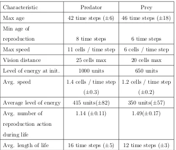
Characteristic Predator Prey

Max age 42 time steps (±6) 46 time steps (±18)

Min age of

reproduction 8 time steps 6 time steps

Max speed 11 cells / time step 6 cells / time step

Vision distance 25 cells max 20 cells max

Level of energy at init. 1000 units 650 units

Avg. speed 1.4 cells / time step 1.2 cells / time step

(±0.3) (±0.2)

Average level of energy 415 units(±82) 350 units(±57)

Avg. number of 1.14 (±0.11) 1.49(±0.17)

reproduction action

during life

Avg. length of life 16 time steps (±5) 12 time steps (±3)

Table 3.1: Several physical and life history characteristics of individuals from 10

independent runs.

3.2 Entities, state variables, and scales

Individuals: EcoSim has two types of individuals: predator and prey. Each

in-dividual possesses several characteristics (Table 3.1) such as: age, minimum age

for breeding, speed, vision distance, level of energy, and amount of energy

trans-mitted to the offspring. Energy is provided to the individuals by the resources

(food) they find in their environment. Prey consumes grass, which is dynamic in

quantity and location, whereas predator hunts for prey individuals. Each

indi-vidual performs one unique action during a time step, based on its perception of

the environment. Each agent possesses its own FCM that represents its genome

and also its behaviors are determined by the interaction between the FCM and

the environment. Thus, the FCM allows flexibility in behavioural responses to the

changing environment, but since the FCM has fixed values at birth it does not

model plasticity in the conventional sense (the FCM is discussed in detail below).

(38)

environment. For example, prey individuals gain 250 units of energy by eating

one unit of grass and predators gain 500 units of energy by eating one prey. At

each time step, each agent spends energy depending on its action (e.g. breeding,

eating, running) and on the complexity of its behavioral model (number of existing

edges in its FCM). On average, a movement action such as escape and exploration

requires 50 units of energy, a reproduction action uses 110 units of energy and the

choice of no action results in a small expenditure of 18 units of energy.

Cells and virtual world: The virtual world is discrete and consists of a matrix

of 1000*1000 space units called cells. Each cell represents a large space which

may contain an unlimited number of individuals and/or some amount of food.

The world is large enough in order to observe migration patterns, an individual

moving in the same direction during its whole life cannot even cross half of the

world, making large-scale migrations possible. The virtual world wraps around to

remove any spatial bias. In addition, the dimensions of the world are adjustable

but increasing the dimensions can increase the computation complexity of the

simulation by allowing more individuals to co-exist.

Time step: Each time step involves the time needed for each agent to perceive

its environment, make a decision, perform its action, as well as the time required

to update the species membership, including speciation events and record relevant

parameters (e.g. the quantity of available food). In terms of computational time,

the speed of simulation per generation is related to the number of individuals.

Recent executions of the simulation produced approximately 15 000 time steps in

35 days.

Population and Species: In average in every time step of the simulation, there

are 250,000 individuals which consisting of one or more species. A species is a set

of individuals with similar genome.

3.3 Process overview and scheduling

The possible actions for the prey agents are: perceive the environment to obtain

information of the vicinity in terms of grass, predators, and sexual partner, evasion

(39)

the its habitat cell, prey can move to another cell to find grass), socialization

(moving to the closest prey in the vicinity), exploration, resting (to save energy),

eating and breeding. Predator also perceive the environment to gather information

used to choose an action among: hunting (to catch a prey), search for food,

socialization, exploration, resting, eating and breeding. For every individual the

energy is adjusted after an action is performed at each time step. The age of every

individual is also updated at each time step (age is simply the number of time steps

until an individual dies). There are also two environmental processes that depend

on the actions of prey and predators, the amount of grass which is consumed by

prey and meat which is consumed by predators, which are also adjusted at each

time step. At each time step, the value of the state variables of individuals and

cells are updated. The overview and scheduling of every time step is shown in

Fig.3.1.

The complexity of the simulation algorithm is mostly linear in the number of

individuals. If we consider that there are N1 preys and N2 predators then the

complexity of part 1 and part 2of the above algorithm, including the clustering

algorithm used for speciation, will be O(N1) and O(N2) respectively ([58]). This

virtual world of the simulation has 1000*1000 cells, therefore the complexity of

part 3 will be O(k = 1000*1000). The complexity of part 4 will be O(N1+N2).

As a result the overall complexity of the algorithm will be calculated as O(2N1+

2N2+ k), which is O(N = 2N1 +2N2).

3.4 Design concepts

3.4.1 Basic principles

In EcoSim, a FCM is the base for describing and computing the agent behaviors.

Each agent possesses a unique FCM to compute its next action. Their FCM is

represented in their genome which is assigned to each individual at birth. A FCM

is a directed graph containing nodes representing concepts and edges representing

the influence of concepts on each other (Fig.3.2). When a new offspring is created,

(40)

(41)

possible mutations. Formally, an FCM is a graph which contains a set of nodes C,

each node Ci being a concept, and a set of edges I, each edge Iij representing the

influence of the concept Ci on the concept Cj. A positive weight associated with

the edge Iij corresponds to an excitation of the concept Cj from the concept Ci,

whereas a negative weight is related to an inhibition (a zero value indicates that

there is no influence of Ci on Cj). The influence of the concepts in the FCM can

be represented in an nn matrix, L, in which Lij is the influence of the concept Ci

on the concept Cj. If Lij = 0, there is no edge between Ci and Cj.

3.4.2 Emergence

In each FCM, three kinds of concepts are defined: sensitive (such as distance to foe

or food, amount of energy, etc.), internal (fear, hunger, curiosity, satisfaction, etc.),

and motor (evasion, socialization, exploration, breeding, etc.). The activation level

of a sensitive concept is computed by performing a fuzzification of the information

the individual perceives in the environment. For an internal or motor concept C,

the activation level is computed by applying the defuzzification function on the

weighted sum of the current activation level of all the concepts having an edge

directed toward C.

Finally, the action of an individual is selected based on the maximum value

of motor concepts’ activation level. Activation levels of the motor concepts are

used to determine the next action of the individual. For example in Fig.3.3.

there are two sensitive concepts (foeClose (predator close) and foeFar (predator

far)), one internal (fear), and one motor (evasion). There are also three influence

edges: closeness to a foe excites fear, distance to a foe inhibits fear, and fear

causes evasion. Activations of the concepts foeClose and foeFar are computed by

fuzzification of the real value of the distance to the foe, and the defuzzification

of the activation of evasion tells us about the speed of the evasion. The values

of edges for each individual are fixed throughout his life, and are combined with

another individual with possible mutation when forming a new offspring.

At the initiation of the simulation prey and predators scattered randomly all

(42)

Figure 3.2: Initial FCM prey map including concepts and edges. The width of

each edge represents the influence value of a concept on another. Color of an edge

shows inhibitory (red) or excitatory (blue) effects.

Figure 3.3: An FCM for detection of foe (predator) and decision to evade with

its corresponding matrix (0 for ’Foe close’, 1 for ’Foe far’, 2 for ’Fear’ and 3 for

(43)

the individuals in the world is changed drastically based on many different factors:

prey escapes from predators, individuals socialize and form groups, individuals

migrate gradually to find sources of food, species emerge, etc. Fig.3.4 and Fig.3.5

show an example of a snapshot of the virtual world after thousands of time steps

with emerging grouping patterns of species and grass distribution respectively.

It has been shown that the data generated by EcoSim present the same kind of

multifractal properties as the ones observed in real ecosystems [59]. Individuals’

distribution forming spiral waves is one property of prey-predator models. The

prey near the wave break has the capacity to escape from the predators sideways.

A subpopulation of prey then finds itself in a region relatively free from predators.

In this predator-free zone, prey starts expanding intensively and form a circular

expanding region. The whole pressure process and spiral formation will be applied

to this subpopulation of prey and predators again leading to the formation of the

second level of spiral [60]. Because there are consecutive interactions between

prey and predators during time, the same pattern repeats over and over and then

self-similarity emerges in spatial distribution of individuals which is a common

property of self-similar processes [61]. As can be seen in the figure individuals

grouped together, and different species emerged. In addition migration phenomena

can be observed, as relocation of the individuals leads to the redistribution in the

population.

3.4.3 Adaptation

The genome maximal length is fixed (390 sites), where each site corresponds to an

edge between two concepts of the FCM. But, as many edges have an initial value

of zero, only 114 edges for prey and 107 edges for predators exist at initialization.

One more gene is used to code for the amount of energy which is transmitted

for the parent to their child at birth. The value of a site (gene), which is a real

number, corresponds to the intensity of the influence between the two concepts.

The genome of an individual is transmitted to its offspring after being combined

with the one of the other parent and after the possible addition of some mutations.

(44)

Figure 3.4: The snapshot of the virtual world in one specific time step, white color

(45)

Figure 3.5: The snapshot of the virtual world for a specific time step of the

genomic and behavioural evolution in the artificial ecosystem simulation EcoSim

Scholarship at UWindsor

Scholarship at UWindsor

genomic and behavioural evolution in the artificial ecosystem

genomic and behavioural evolution in the artificial ecosystem

simulation EcoSim

simulation EcoSim

Genomic and behavioural evolution in the

artificial ecosystem simulation EcoSim

Marwa Fouad Khater

Contents

List of Tables

List of Figures

Chapter 1

Introduction

1.1

Motivation

1.2

Objective

1.3

Contributions of the thesis

1.4

Outline of thesis

Chapter 2

Background and Literature

Review

2.1

Artificial life

2.2

IBM

2.2.1

Tierra

2.2.2

Avida

2.2.3

Echo

2.2.4

Polyworld

2.2.5

Framsticks

2.3

Other predator-prey simulations

Chapter 3

Individual based ecosystem

simulation EcoSim

3.1

Purpose

3.2

Entities, state variables, and scales

3.3

Process overview and scheduling

3.4

Design concepts

3.4.1

Basic principles

3.4.2

Emergence

3.4.3

Adaptation