Optimal Sensor Deployment in Homogeneous
&Heterogeneous Wireless Sensor Network
Komal Sunil Khamkar, Prof. Nighot Mininath K.
ME Student, Department of Computer Engineering, K. J. College of Engineering and Management Research, Savitribai
Phule Pune University Pune India.
Professor, Department of Computer Engineering, K. J. College of Engineering and Management Research, Savitribai
Phule Pune University Pune India.
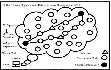
ABSTRACT: Optimal sensor deployment is necessary for homogeneous and heterogeneous wireless sensor deployment. It recommends to spatial communication among wireless sensor nodes and its intermediate node. Currently sensor deployment strategy leads towards more delay in packet transmission in wireless network. In order to resolve minimum cost for packet transmission proposed system design an approach of optimal sensor deployment. Which present an idea for implementing optimal sensor deployment in homogeneous and heterogeneous wireless networks. Proposed approach implements a Restrained Lloyd (RL) algorithm and a Deterministic Annealing (DA) algorithm to optimize sensor deployment in both homogeneous and heterogeneous WSNs. This paper also investigates a dynamic deployment using non-uniform sensor densities to gain energy consumption balance and maximize network lifetime. This can be achieved by First Order Radio Model where Movement algorithm is used for optimal sensor deployment to balance energy resource. Sensor nodes can move several times where network life time in divided into some rounds. Proposed simulation result shows that network lifetime can be improved in both homogeneous and heterogeneous wireless network. The deployment and topology control of such heterogeneous WSNs that involve the sensor nodes with different communication or sensing area have been manipulated. Furthermore, proposed system makes enhance work by multiple sink nodes in wireless sensor network. Location wise predetermined sensor deployment. The simulation results show that proposed sensor deployment technique does not com-promise with other performance metrics like end-to-end delay and throughput, while obtaining the proposed solution. Finally, all the comparative results show that this scheme is supremacy over the competing systems.
KEYWORDS: Sensor deployment, DA, RL.
I. INTRODUCTION
Wireless sensor networks (WSNs) gather information from the wireless network deployed in the environment and sends to virtual information world, such as computers. Appropriate wireless sensor deployment improves monitoring and controlling the networks environment. To achieve their tasks, WSNs need to solve two requirements like
(i) Sensing in the target area and
(ii) Communication between the sensor nodes.
are used in WSNs. This work implements a dynamic deployment using non-uniform sensor network to achieve energy balance and longer network lifetime. Different from the previous study, the sensor placement is dynamic which can change the sensor densities according to application. A mathematical model is proposed to synthesis the expected sensor density in the monitored area. Here, first introduce the system model for both homogeneous and heterogeneous WSNs and formulate the problems of sensing and connectivity. The density requirement may also change after a network has been created due to changes in application modes or environmental conditions. Some regions may create or transmits more packets than others for some needful events still their locations are not near the sink node. For example, after an intruder is detected, the region in the location of the intruder may generate more messages. Proposed system develops a model which provides minimum distortion with Maximum Coverage. We develop node deployment strategy in Dimensional environment. By considering node deployment we can deploy maximum number of sensor nodes in a limited range that results in optimization of network lifetime. This work can derive number of homogeneous and heterogeneous sensors to be deployed along with their deployment region. Deployment system in WSN explore each sensor node sends its data to the relay node having maximum energy and then it is send to the nearest sink node of the WSN.
II. REVIEW OF LITERATURE
A proposed system emphasizes the literature study of different sensor node deployment methods are defined In [2] this researcher have introduced the maximum coverage for network deployment problem in wireless sensor networks and reasons of properties of the problem and its solution space. This work proposes an efficient genetic algorithm with a novel normalization method. To cover a wide range of a target area with a minimum number of sensors and can be accomplished by efficient deployment of the sensors. Sensor coverage models measure the sensing capability and quality by capturing the geometric relation between a point and sensors. An approach to find out least covered regions in a sensor network where further sensor deployment is expected.
In [3] this work researcher tackles the problem of optimal surface deployment problem on 3D surfaces, aiming to achieve the highest overall sensing quality. It introduces a new model to formulate the problem of sensor deployment on 3D surface. It considers stationary and homogeneous sensors deployed on surfaces. The accuracy of their gathered information based on the distance between the sensor and the destination point to be sensed. It presents the optimal solution for 3D surface sensor deployment with minimized overall unreliability.
In [4] Researcher determines the optimal deployment of nodes by taking into consideration the density in monitored area. By using this dynamic deployment scheme, energy balance can be achieved. A mathematical model is proposed to compute the desired sensor density in the monitored area. Sensor nodes send their messages to a sink located centrally. The density distribution optimization problem is solved by determining number of nodes in each sub-region as a result, longer lifetime is achieved.
In [5] researcher proposed techniques for balanced energy depletion for a primitive geometric node distribution (GND) and a primitive energy proportional node distribution (EPND). Three novel non uniform node distribution strategies are proposed. Strategy I is able to fully achieve energy balance. Strategy II achieves the longest network lifetime through the EPND and a simple sensing/ non sensing switch scheduling. Strategy III requires the fewest sensor nodes among the three proposed strategies.
The distributed wireless video scheduling with delayed control information (DCI) is proposed in [6]. It considers two classes of DCI distributions first the class with finite mean and variance and second is a general class that does not employ any parametric representation. A distributed scheduling scheme is proposed to achieve performance bound by making use of the correlation among the time-scale control information.
balancing and enhancing network lifetime. Node deployment using Gaussian distribution is widely acceptable when random deployment is used.
Optimal Sensor deployment together with a realistic terrain model is proposed in [8]. It assumes only those terrain features which can be modeled by convex polygons. Optimal sensor deployment together with a realistic terrain model makes sensor deployment more practical and robust. Results show that the number of sensors, their locations and the node density change in presence of obstacles.
In [9] researcher proposed a curve based sensor deployment for coverage barriers in WSN. For improving barrier coverage performance, we introduced a concept of distance-continuous curve, and provided an algorithm to obtain the optimal sensor deployment when the deployment curve is distance continuous, and an algorithm which can attain close-to-optimal sensor deployment when the deployment curve is not distance continuous.
Two deployments strategies-Hexagonal Deployment Strategy (HDS) and Diamond Deployment Strategy (DDS) are proposed in this system [10]. A Radar Sensor Network (RSN) is efficiently deployed to find multi-target within a given network deployed area with required detection performance and energy consumption. It propose two decision fusion rules over pass-loss fading channel in multi-hop RSN to improve the performance of multi-target detection.
In [12] described the sensor deployment problem as a source coding problem with distortion reflecting sensing accuracy. When the communication range is limited, a WSN is divided into several disconnected sub-graphs under the condition that every sensor node location should coincide with centroid of its own optimal sensing region. In this a backbone network is designed for communication between sensor nodes and cluster node in the wireless sensor or mobile adhoc network [12].
III. SYSTEM ARCHITECTURE
Proposed optimal sensor deployment provides the use of our RL Algorithm. The algorithm implemented in between two steps: (i) Sensors in the backbone network move one by one. Each sensor in the base network calculates its own approximate desired region Li (P) and moves to a critical location with maximum local performance. Sensors outside the backbone network move randomly and check if there is a path to the AP. Unlike the conventional Lloyd algorithm, these new locations may not be the centroid of the partition regions; (ii) The target area, Q, is partitioned to WVDs for sensors in the backbone network, S(P). The final distortion only considers sensors in the backbone network. Initially, two strong sensors and four weak sensors are consisted in the backbone network.A Sensor Nodes in network chooses a Relay Nodes as a receiver which is nearest to SN and has the highest residual energy for sending its data. If there is more than one receiver node with the same highest residual energy, one of them is chosen randomly. Next, the receiver RN employs the same procedure to choose the next receiver RN in the network for sending its data. This process repeats till the data arrives at the sink node.
IV. MATHEMATICAL MODEL
Sensor nodes are distributed within two dimensional region covered by a set of regular hexagonal cells. The network coverage area (ab) is divided into N number of layers and each layer is divided into M number of RHCs with radius r. In every a layer where i=1 N. A layer is called either odd or even based on the value of i. For example, are the even layers whereas are the odd layers. Further, the sink is assumed to be located at one corner of the network area and responsible for collecting imagery data from the SNs. A RHC in the network is identified by (where i=1,, N and for each i, j=1,,M) which indicates the jjiCth cell in layer-i. For example, the RHC identifies the 224Cnd cell in layer-4. Here, i=1 indicates the layer nearest to and i=N indicates the layer farthest from the sink, whereas j=1 indicates the cell nearest to and j=M indicates the cell farthest from the sink within a layer. Bi is defined as the boundary between two
consecutive layers- layer-i and layer-(i+1).
For target tracking sensor deployment in wsn Euclidean distance between points p and q is the length of the line segment between two sensor points. A vector can be described as a directed line segment from the origin of the Euclidean space (vector tail), to a point in that space (vector tip). If we consider that its length is actually the distance from its tail to its tip, it becomes clear that the Euclidean norm of a vector is just a special case of Euclidean distance: the Euclidean distance between its tail and its tip. The distance between points p and q may have a direction (e.g. from p to q), so it may be represented by another vector, given by Shortest Distance Calculation In proposed Radio Resource Controlling model designed to implement energy efficient wireless communication by shortest path routing.
Proposed shortest path routing uses Euclidean distance between two sensor is calculated using Distance
((x, y), (a, b)) = ( − )² + ( − )²
Where, Distance between two sensor node using their lon-gitude and latitude that is x as longitude and y as latitude for first node and a is longitude and b is latitude for second node in mobile sensor nodes. Euclidean formula gives the distance for one to every another sensor in the same cluster for energy efficient packet transmission.
Throughput, or flow rate, is a calculation is used in operations management that allows a simulation to find what their output is in a given amount of time. This output can be in either a packet transmission time in network. The formula is based on Little’s Law, which in essence is used to calculate the average number packet transmission in a stipulated amount of time. When the nodes are rearranged,
TH = I / T
TH is the throughput that proposed system calculated, or the average output of packet transmission within stipulated amount of time.
T is the total time that is required to complete packet trans-mission time.
A. Algorithms :
1. Steps Target Localization in to deploy sensor
Set loops=0;
Set MaxLoops=MAXLOOPS;
While(loops <maxLoops)
ForP (x; y)inHexGrid; x[a; width]; y[1; height] Forsis1; s2; s3:sk
CalculateCxy(Si; P )fromthesensormodel Using(d(si; P ); cth; dth; ; );
End IfcoveragerequirementaremetBreakwhileloop
End
End
Forsis1; s2; ;sk
CalculateFijusingd(si; sj); dth; wA; wR; CalculateFiAusingd(si; PA1; ; PAnP ); dth; CalculateFiRusingd(si; OA1; ; OAnO); dth; Fi = Fij + FiR + FiA; j[1; k]; j = i;
End
Forsis1; s2; ;sk Fi(si)virtuallymovessitoitsnextposition; End
Setloops = loops + 1; End
2. Sensor deployment in 3D by multi objective 3D environment
1:Initial Sensor deployment;
2: Determine the best individuals best1 best2 according to
objective1 objective2;
3:Divide the population into two sub-populations;
4:For each sub population do
Determine the fitness of each
Individual according to
Corresponding objective;
5:Roulette wheel selection for each sub population;
6: Combine and alter sub populations into temporary population 7:Perform recombination on temporary population
8:Perform mutation on temp-population;
9:Next generation= temp-population;
10: Inject best1 and best2 individuals into the next generation;
11: If stop criteria is not satisfied, Go to step 2;
12: Show results for objective1 objective2
3.Routing Algorithm:-
// on receiving ENERGYQUERYM SGfromnodei1 : ifisRN(i)then
2 :AckEnergyInfo(ID);
3 : else
4 :DiscardMsg;
5 :endif
==onreceivingaDATAF ORWARDMSGfromnodej6 : k = SelectNextRN(q)
7 :ifIsRN(j) == TRUEthen
8 : Send(k; DATAF ORWARDM SG(data)) 9 : else
10 :DiscardMsg;
11 :endif ==onreceivingnomessage
12 : k = SelectNextRN(q);
13 : Send(k; DATAF ORWARDMSGk(selfdata))
V. SYSTEM OVERVIEW
A. Software Requirement Specification
1. Design Wireless sensor Network as Simulation
2. Determine network communication type i.e. Heterogeneous and Homogeneous.
3. Prepare routing table for prescribed source and destination.
4. Selection of optimal sensor nodes for energy efficient communication.
5. Optimal sensor deployment in WSN.
6. Heterogeneous and homogeneous sensors communication.
9. Secure routing by appropriate key management i.e. public key cryptography.
10. Energy efficient packet transmission.
In proposed work is designed to implement above software requirement. To implement this design following software requirements are used.
B. Platform
Operating System: Windows7
Front End : Java Swing (Simulation)
Tool : Eclipse Luna
C. Outcomes and success
Proposed system is designed using java swing component as simulator. Optimal sensor deployment is designed for maximize end to end throughput by reducing communication overhead in wireless sensor network. Proposed system achieves great performance for packet transmission in network.
E. Comparison with similar System
VI. RESULT ANALYSIS
Optimal sensor deployment in dynamic wireless sensor network expected to explore simulation in the form of minimal sensor deployment evolve to maximize throughput in wireless packet transmission. Proposed system is expected node deployment with LIoyd Algorithm in shown in following figure2. Optimal sensor deployment improves the throughput for packet transmission, Optimal sensor deployment. Proposed predetermined sensor deployment leads to reduce delay for packet transmission.
Fig. 3. Sensor Deployment
In this section performance metrics are use d to evaluate performance of routing protocols and data dissemination protocols scheme when no in networking processing is performed and no caching is used.
VII. PERFORMANCE MEASURES
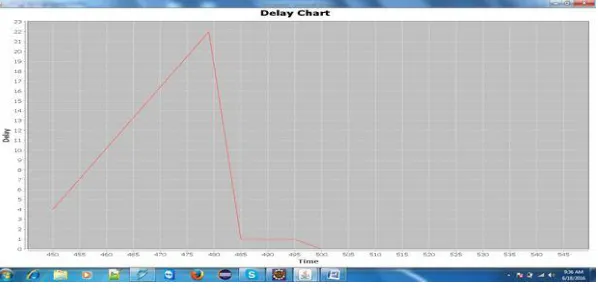
A. Delay Chart
This measure is used to reduce packet transmission in wireless sensor network or mobile adhoc network along
B. Throughput Maximization:-
C. Packet Delivery Ratio:-
Proposed wireless sensor network designed to improve packet delivery ratio at end to end sensor nodes. This measure verifies against packet loss during wireless communication between source nodes.
VIII. CONCLUSION
In dynamic wireless sensor network the deployment of sensors for three types of network in heterogeneous wireless sensor networks. The optimal sensor deployment and gradient are provided to finds optimal sensor locations. Proposed model permits network deployment to find the most efficient density for sub-region to achieve energy balance and maximize thelifetime of network. Proposed system achieve target of network lifetime improvement by optimal sensor node deployment. Proposed movement algorithm tends to deploy sensors in limited area range so that they improve efficiency in both heterogeneous and homogeneous wireless communication.Proposed optimal sensor deployment does not limit transmission coverage area for sensor nodes. Clustering is techniques are used for energy efficient packet transmission in un limited transmission range.
ACKNOWLEDGMENT
The authors would like to thank. The preferred spelling of the word ”acknowledgment” in America is without an ”e” after the ”g”. Avoid the stilted expression ”one of us (R. B. G.) thanks ...”. Instead, try ”R. B. G. thanks...”. Put sponsor acknowledgments in the unnumbered footnote on the first page.
REFERENCES
[1] S. Halder and A. Ghosal, A Location-wise Predetermined Deployment for Optimizing Lifetime in Visual Sensor Networks, IEEE Transactions on Circuits and Systems for Video Technology,2015.
[2] M. O. Rahman, M. A. Razzaque, and C. S. Hong, Probabilistic Sensor Deployment in Wireless Sensor Network: A New Approach, International Conference on Advanced Communication Technology, vol. 2, pp. 1419-1422, 2007.
[3] M. Jin, G. Rong, H. Wu, L. Shuai, and X. Guo, Optimal Surface Deployment Problem in Wireless Sensor Networks, Proceedings IEEE-INFOCOM, pp.2345-2353, 2012.
[4] Y. Xu, L. Shen and Q. Yang, Dynamic Deployment of Wireless Nodes for Maximizing Network Lifetime in WSN, International Conference on Wireless Communications Signal Processing, 2009.
[5] H.W. Ferng, M. S. Hadiputro and A. Kurniawan, Design of Novel Node Distribution Strategies in Corona-Based Wireless Sensor Networks, IEEE Trans. on Mobile Computing, vol. 10, no. 9, pp. 1297-1311, 2011.
[6] L. Zhou, Z. Yang, Y. Wen, and J. J. P. C. Rodrigues, Distributed Wireless Video Scheduling with Delayed Control Information, IEEE Trans. on Circuits and Systems for Video Technology, vol. 24, no. 5, pp. 889-901, 2014.
[7] S. Halder, and A. Ghosal, Is Sensor Deployment using Gaussian Dis-tribution Energy Balanced?,Proc. of 13th Intl Conf. on Algorithms and Architectures for Parallel Processing (ICA3PP),LNCS, vol. 8285, pp. 58-71, 2013.
[9] S. He, X. Gong, J. Zhang, J. Chen and Y. Sun, Curve-Based Deployment for Barrier Coverage in Wireless Sensor Networks, IEEE TRANS-ACTIONS ON WIRELESS COMMUNICATIONS, VOL. 13, NO. 2, FEBRUARY 2014.
[10]L. Yang, J. Liang and W. Liu, Radar Sensor (RS) Deployment for Multi-Target Detection, Sixth International Conference onWirelessCommuni-cations and Signal Processing (WCSP), 2014.
[11]Y. Yoon and Y.H. Kim, An Efficient Genetic Algorithm for Maximum Coverage Deployment in Wireless Sensor Networks, IEEE Transactions on Cybernetics, 2013.