Improved Real Time Predictive Speed Analysis for High Speed Rail Collision Test

Scholarship at UWindsor

Scholarship at UWindsor

Electronic Theses and Dissertations Theses, Dissertations, and Major Papers

2016

Improved Real Time Predictive Speed Analysis for High Speed Rail

Improved Real Time Predictive Speed Analysis for High Speed Rail

Collision Test

Collision Test

Bo Yu

University of Windsor

Follow this and additional works at: https://scholar.uwindsor.ca/etd

Recommended Citation Recommended Citation

Yu, Bo, "Improved Real Time Predictive Speed Analysis for High Speed Rail Collision Test" (2016). Electronic Theses and Dissertations. 5922.

https://scholar.uwindsor.ca/etd/5922

This online database contains the full-text of PhD dissertations and Masters’ theses of University of Windsor students from 1954 forward. These documents are made available for personal study and research purposes only, in accordance with the Canadian Copyright Act and the Creative Commons license—CC BY-NC-ND (Attribution, Non-Commercial, No Derivative Works). Under this license, works must always be attributed to the copyright holder (original author), cannot be used for any commercial purposes, and may not be altered. Any other use would require the permission of the copyright holder. Students may inquire about withdrawing their dissertation and/or thesis from this database. For additional inquiries, please contact the repository administrator via email

Analysis for High Speed Rail Collision

Test

By

Bo Yu

A Thesis

Submitted to the Faculty of Graduate Studies through the School of Computer Science in Partial Fulfillment of the Requirements for

the Degree of Master of Science at the University of Windsor

Windsor, Ontario, Canada

2016

c

by

Bo Yu

APPROVED BY:

Dr. Chunhong Chen

Department of Electrical and Computer Engineering

Dr. Arunita Jaekel School of Computer Science

Dr. Dan Wu, Advisor School of Computer Science

I hereby certify that I am the sole author of this thesis and that no part of this

thesis has been published or submitted for publication.

I certify that, to the best of my knowledge, my thesis does not infringe upon

anyones copyright nor violate any proprietary rights and that any ideas, techniques,

quotations, or any other material from the work of other people included in my

thesis, published or otherwise, are fully acknowledged in accordance with the standard

referencing practices. Furthermore, to the extent that I have included copyrighted

material that surpasses the bounds of fair dealing within the meaning of the Canada

Copyright Act, I certify that I have obtained a written permission from the copyright

owner(s) to include such material(s) in my thesis and have included copies of such

copyright clearances to my appendix.

I declare that this is a true copy of my thesis, including any final revisions, as

approved by my thesis committee and the Graduate Studies office, and that this thesis

In real train collision test, the test train cabin is required to be propelled on a

straight rail, accelerated to a certain velocity, released at a calculated location and

finally crash into a barrier with a desired crash velocity, in order to observe the safety

performance. Recently, a Real Time Predictive Speed Analysis (RTPSA) method was

developed to simulate the whole collision test behavior and calculates the released

velocity and location. However, in this method, the train has to be released at the

exact calculated velocity when the train is still in acceleration which is very difficult

in real test. Moreover, the RTPSA method does not provide a warning mechanism

in case the test has to be aborted. In this thesis, two improvements of the RTPSA

method are proposed. One is employing the PI controller to force the train operating

with an uniform velocity before release, in order to reduce the difficulty of release

in real test. The other one is early safety warning which provide upper bound of

velocity, before the test, indicating the last chances to abort the test with least losses

I would like to present my gratitude to my supervisor Dr. Dan Wu for his valuable

assistance and support.

I also would like to express my appreciation to Dr. Chunhong Chen and Dr.

Arunita Jaekel. Thank you all for your valuable comments and suggestions to this

thesis.

Meanwhile, I want to thank my lab-mates for helpful discussions and advice.

Finally, I thank my parents, my girlfriend and my friends who give me consistent

DECLARATION OF ORIGINALITY III

ABSTRACT IV

AKNOWLEDGEMENTS V

LIST OF TABLES VIII

LIST OF FIGURES IX

I Introduction 1

1 Introduction of High Speed Rail . . . 1

2 History of HSR . . . 2

3 Safety Issues and Solutions . . . 3

4 Motivation . . . 4

5 Contributions . . . 5

6 Guide to the Thesis . . . 6

II Background Knowledge 7 1 Real Collision Test . . . 7

1.1 Test Process . . . 7

1.2 Test Facility . . . 8

2 RTPSA . . . 10

2.1 Data Source . . . 10

2.2 Coefficients Calculation Module . . . 12

2.3 Coast-Down Simulation Module . . . 14

2.4 Propulsion Simulation Module . . . 16

2.5 Control/Release Module . . . 17

2.6 Summary . . . 18

3 PID Controller . . . 19

3.1 Proportional Term . . . 20

3.2 Integral Term . . . 21

3.3 Derivative term . . . 22

3.4 Tuning Coefficients . . . 22

3.5 Summary . . . 22

III Limitation of RTPSA 24 1 Early Safety Warning . . . 24

1.1 Necessary Simulation Before Real Test . . . 29

1.2 Feasibility of the Calculation Based on Simulated Data . . . . 32

2 Software Structure . . . 33

3 Early Safety Warning Module . . . 35

3.1 Principle and Design . . . 35

3.2 Program Logic . . . 44

4 PID Controller Module . . . 46

4.1 Principle and Design . . . 46

4.2 Program Logic . . . 50

5 Summary . . . 51

V Experiment Results 52 1 The Demonstration . . . 52

2 Experimental Results of LCAand LCR . . . 55

2.1 Different Crash Velocities . . . 55

2.2 Different Barrier Locations . . . 55

2.3 Different Safety Distance . . . 56

3 Comparison of Different PID Configuration . . . 57

3.1 Different Sets of Coefficients . . . 57

3.2 Different Sampling Frequency . . . 60

4 Results of the Improved RTPSA in Different Situations . . . 61

4.1 Real Crash Velocity . . . 61

4.2 Results of Different Crash Velocity . . . 63

4.3 Result of Different Barrier location . . . 64

4.4 Result of Different Safety Distance . . . 65

VI Conclusion 66

REFERENCES 67

1 The results of LCAand LCR based on different crash velocities. . . . 55

2 The results of LCAand LCR based on different barrier locations. . 56

3 The results of LCAand LCR based on different safety distances. . . 56

4 The results of different PID coefficients. The unit of velocity is kmph. 58 5 The results based on different sampling frequency. . . 60

6 The results based on different crash velocities. . . 64

7 The results based on different barrier locations. . . 64

1 Three phases of the collision test. . . 8

2 Test facility one[18]. . . 8

3 Test facility two[18]. . . 9

4 Test facility three[18]. . . 9

5 Data for simulation[18]. . . 11

6 Coefficient module, from A to C[18]. . . 13

7 Coast-down module, from B to D[18]. . . 15

8 Propulsion module, from C to B[18]. . . 17

9 Safety warning information, schematic diagram. . . 25

10 Deviation of simulated release point from real release point, schematic diagram. . . 27

11 The behaviour of the test train in improved RTPSA, schematic dia-gram. . . 28

12 Effect of proportional gain, schematic diagram[5]. . . 30

13 Structure of original RTPSA[18]. . . 33

14 Structure of improved RTPSA. . . 34

15 Parameters in LCA, schematic diagram. . . 36

16 Same image as Figure 15. . . 39

17 Parameters in the second part of early safety warning module, schematic diagram. . . 41

18 Uniform motion in original RTPSA, schematic diagram. . . 44

19 Flow chart of safety warning module. . . 45

20 The simulation model in Simulink, Matlab. . . 48

21 The structure of tuning module. . . 49

22 Parameters for PID module in simulink. . . 49

25 Important information in improved RTPSA. . . 54

26 Response time and transient behaviour in the tuning module. . . 58

27 Performance of different combination of PID coefficients. . . 59

28 Performance of different sampling frequency. . . 61

Introduction

1

Introduction of High Speed Rail

The High Speed Rail(HSR) is a rail transport technology which provides

signifi-cantly faster speed than the traditional rail transport. As the definition of the HSR

is not rigid, the lines operating from 160 km/h to, even more that, 250 km/h can be

regarded as HSR[4].

Japan is the first country opening the HSR system to the public in 1964, in other

words,this HSR system is in operation for around 50 years and carries more than

9 billion people in total[17][28]. Nowadays, HSR is operating in more than twenty

countries (including the UK, France, Germany, Belgium, Spain, Italy, Japan, China,

Korea, and Taiwan), while other around 20 countries are developing and constructing

it(such as Turkey, Qatar, Morocco, Russia, Poland,etc.)[6][18].

In terms of the benefits, HSR offers a convenient, comfortable, affordable and

safety choice to travel without delays. Other than this, it relieves the congestion on

local traffics while delivers punctual and fast service to the passengers. Further more,

it is powered by electricity,which as a result significantly reduces the budget on oil

purchase for countries. And it creates plenty of job opportunities constructing the

2

History of HSR

The development of the railway is the development of the speed. In 1829, George

Stephenson created a locomotive reaching 50km/h which represented the high speed

standard of the train at that time[8][15]. However, this record was broken by many

other higher speed at the beginning of the 20th Century.

Although the speed is satisfiying at that time, the development of other transport

modes push the train producers to strengthen the performance of the existing trains.

After a huge speed improvement in Europe, in 1964, Japan impressed the world by

the operation of a fully new standard gauge line, the Tokaido Shinkansen[17]. It was

designed to operate at 210 km/h, with broad loading gauge, electric motor units,

Au-tomatic Train Control (ATC), Centralised Traffic Control (CTC) and other modern

improvements.

After the huge success of Japanese HSR, the European HSR was born in France

between Paris and Lyons in 1981, at a maximum speed of 260 km/h[8]. In addition

to its high speed, the compatibility with the original rail system was considered as

the most important contribution, due to its influence on the future upgrade of the

old railway system.

Based on the experience of HSR in France, many other European countries such as

Germany(in 1988), Spain(in 1992), Belgium(in 1997), the United Kingdom(in 2003)

developed their own high speed railway system[30]. At the same time, China built

the HSR in 2003. Chinese HSR was operating at the average speed of 200kp/h or

even higher[22].

A new step forward for HSR started in China on 1 August 2008, when the 120 km

long high speed rail between Beijing to Tianjin was build[14]. After 2008, China

con-ventional railways and newly built high-speed passenger designated lines (PDLs)[16].

The HSR system in China carries at least 800 million passengers per year ( from 2014

and growing), more than half of the total high speed traffic in the world[3].

3

Safety Issues and Solutions

Because of the increasing speed of HSR, the safety issues turns out to be more

important. On 23 July 2011, a deadly crash happened between two high-speed trains

travelling through Wenzhou, China. Fourty people were killed, and at least 192 were

injured. Based on the official investigation, the accident was blamed for the faulty

signal systems which failed to warn the second train that the first train was on the

same rail[2].

Another serious HSR accident happened in Santiago, Spain, on 24 July 2013. The

train derailed at high speed when turning around on a bend, killing 79 people while

other 140 were injured. The reason was the train exceeded the speed limit(80 km/h)

twice when passing the bend[1].

Many other HSR accidents have not been mentioned here, and due to these

un-expected collisions, a large amount of researchers in the area of HSR focus on safety

issues. Some of the research topics refer to minimizing the human body injury when

train accident occurs.

Due to the danger of high speed train accident, many countries have developed

safety guidelines for the train in the designing phase to improve crashworthiness[26][23][13][29].

In order to test these designs, the real train collision test is required. In a real train

collision test, a test train is accelerated by a propulsion system. After reaching a

cer-tain speed, it will be released and hit the barrier with a desired speed to observe the

crashworthiness. Obviously, the test facilities require massive expense. As a result,

which simulate the entire collision test based on theoretical data[21][20][19].

However, the existing simulation methods process only with the theoretical data

and past experience, which can not completely study the behaviour of the test train

in real test[24][27]. Thus, a recent method called Real Time Predictive Speed

Anal-ysis(RTPSA) will be discussed in this thesis. Different from previous simulation

methods, RTPSA is a real time method implemented in a real collision test. RTPSA

can analyse the effects of the factors which are difficult to be included by the

tradi-tional simulation methods as they are changing all the time and can not be predicted,

such as the resistance of the air[18].

RTPSA firstly applies a regression analysis model to study the real time

perfor-mance of the testing train, consisting of forces, velocity and location, which can be

collected by the sensors. After some calculation, the relation between resistance and

velocity is found and represented by an expression. Later on, this relation is used

to predict the movement of the train, in order to find out the release velocity and

location before the test train reaches this release point. And then, the test train can

crash into the barrier with the desired velocity, if it is released at this release point.

More details of RTPSA will be introduced in chapter 2.

4

Motivation

For study purpose, RTPSA is only implemented with simulated data. Although

RTPSA operates as expected with simulated data set, there are still two important

disadvantages.

The first disadvantage is lack of early safety warning for aborting the test.

Ex-ception may happen during the test and sometimes it is necessary to abort the test.

Once the train is propelled by the propulsion cart, both the propulsion cart and the

so that the test vehicle can brake successfully and the barrier is not damaged, the

current RTPSA method has to be augmented with a module that can decide if

abort-ing the test is doable by given the velocity of the train, and the distance travelled so

far.

Another disadvantage is the difference between the predicted release point

ob-tained by RTPSA and the real release point. This difference is caused by the

unsuffi-cient simulated method utilized by RTPSA when predicting the behaviour of the test

train, which will be mentioned in detail in chapter 3. Due to this reason, the train

can not be released precisely, therefore required to be improved. And the improved

method will be simply mentioned in next section and discussed in detail in chapter 4.

5

Contributions

The thesis focuses on solving the two disadvantages mentioned in the previous

section.

The first contribution is a new additional functionality providing last chances to

abort the test with least money losses in two different conditions. One is before

re-lease, in other words, the test train is connected with the propulsion cart. In this

scenario, the system will offer a solution for stopping the test train and propulsion

cart safely before they strike the barrier. The other condition is the test train has

already been released. Thus, it can not be prevented to hit the barrier, when only

the propulsion cart can be protected. In other words, this condition decides when is

the last chance to release, otherwise the propulsion cart is not safe.

The other contribution, which is also the primary one, is forcing the test train

to do the uniform motion before release, in order to reduce the negative influence

velocity and location) and the “last chance” information from previous contribution,

the new release velocity is obtained and applied as the input of the PID method. PID

method controls the velocity of the propulsion cart, forces it doing uniform motion

with the new release velocity until the test train disconnects with the propulsion

system. More details of the PID method and the system’s design will be introduced

in chapter 2 and 4.

6

Guide to the Thesis

This thesis is organized as following.

In chapter 2, the background knowledge underlying the proposed method will be

reviewed. The chapter 3 presents the drawbacks of the current RTPSA. To solve

these problems, the new method is introduced and broke down into details in chapter

4. And then, the comparisons and improvements can be observed from the running

Background Knowledge

This chapter reviews the background knowledge of the proposed method in this

thesis. Typical setup in real collision test will be briefly reviewed. After that, the

RTPSA method will be broken down into five sections and introduced. And finally,

the PID controller will be discussed.

1

Real Collision Test

1.1

Test Process

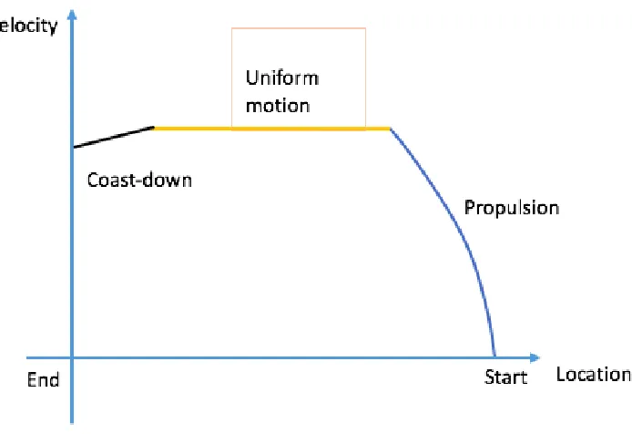
Generally, the real collision test has three phases, which are propulsion phase,

release phase, and coast-down phase. In Figure 1, from top to the bottom, the

first subfigure describes the propulsion phase where the test train is propelled by a

propulsion cart and accelerated from velocity zero. And when reaching the release

velocity/location, the test train will be released immediately in the second subfigure

- release phase. From this time on, in the third subfigure, the test train will be only

affected by the resistance force, thus, coast down towards the barrier, and finally

crash into it. In order to obtain a desired crash velocity, the release velocity/location

is one of the most important factors to be controlled in this test, as the test train can

FIGURE 1: Three phases of the collision test.

1.2

Test Facility

The basic test facility is shown in the following images.

FIGURE 2: Test facility one[18].

In Figure 2, the test train is connected with the propulsion system, located on a

straight guide rail and preparing to be accelerated.

In Figure 3, a rigid wall is located at the end of the rail. And in Figure 4, the

FIGURE 3: Test facility two[18].

2

RTPSA

The previous simulation methods are based on theoretical and historical data.

However, in a real test, resistance forces vary all the time and are subjected to the

velocity of test vehicle, wind speed and direction, temperature and humidity, which

are different in every test. When the collision test is simulated by historical data or

parameters, it brings about less accuracy of the release velocity and location, and

inac-curate crash velocity as well, due to the unpredictable resistance forces. RTPSA(Real

Time Predictive Speed Analysis)is a real-time method (can also process the

simula-tion data) improving the previous ones, which can achieve a more accurate crash

velocity by precisely controlling the release process. The advantage of RTPSA is that

the most up-to-date calibration information can be derived from real-time propulsion

behaviour during the real test[18].

The RTPSA consists of four modules.

• coefficients calculation module

• coast-down simulation module

• propulsion simulation module

• control/release module

At the beginning of the test, RTPSA will collect required data from sensors

de-scribing the behaviour of the test train. And then, the data will feed into coefficients

calculation module for some calculations in order to predict the resistance. Based on

the predicted resistance, the future behaviour of the train can be estimated, and the

release velocity is calculated before the train reaches the release point. More details

are in the following subsections.

2.1

Data Source

In an ideal condition, RTPSA should be implemented in a real test and collect

high expense of a real test .

FIGURE 5: Data for simulation[18].

Figure 5 shows part of the data used for simulation, which is given by Anemoi

Technologies Inc. This dataset is applied in the design stage for studying and

de-bugging purpose. It simulates the beginning propulsion phase by providing the

in-formation of velocity, force, and acceleration based on historical data, which will be

measured by the sensors in a real collision test. At the meantime, the RTPSA is

collecting all these data for the further calculation and simulation in order to predict

the release velocity/location.

In the line “8” of Figure 5, there are three kinds of subscription, which are “a”,

“m” and “c”, indicating three kinds of corresponding data - actual data, measured

data and calculated data. Actual data simulates the real and theoretically

perfor-mance of the system during the propulsion phase. However, due to the mechanical

deviations of the hardware and sensors, the data appeared on the sensors will not be

the actual data exactly, thus, is represented by the so-called measured data. Finally,

In addition, actual data will not be applied, as in real test the available data only

comes from sensors, which is described by the measured data in this dataset. And

later on, this dataset will be collected by RTPSA to predict the behaviour of the test

train.

2.2

Coefficients Calculation Module

This module is a real-time calculating module, in other words, this module will

continuously gather the data from sensors and do calculation while the test train is

propelled. Although, in this research, simulation data replaces the real-time data,

the data will still feed into the module in the same way as in a real test.

This module calculates the necessary coefficients which will be utilized in

predic-tion of the future behaviour of the test train. As introduced previously, the changing

resistance is the reason why most simulation methods can not work accurately. In

principle, the resistance is the combination of two parts, which are friction and

aero-dynamic resistance. Based on the physics of friction and aeroaero-dynamic, the relation

between R and v can be expressed by the following equation,

R =b0v2+b1v +b2 (1)

where b0, b1, b2 are constants, b0v2 +b1v represents the aerodynamic force, b2

cor-responds to the friction. If given a set of data (R, v), the three coefficients can be calculated, and then this relationship can be applied to predict the future behaviour

of the train. The value of v is able to be collected from the sensors, so next question is how to obtain the corresponded resistanceR. Actually, the whole behaviour of the train follows the laws of motion,

F −R=m∗A (2)

Ris calculated and then combined with the corresponded velocityvmeasured at same moments. Thus, a dataset SETRv is gained,

SETRv :{(Rt, vt) :t = 1,2, ..., n}

where R is resistance, v is velocity, and t is the timepoint when sensors do one measurement. With the knowledge of multiple linear regression model and dataset

SETRv, the coefficients b0, b1, b2 are obtained.

FIGURE 6: Coefficient module, from A to C[18].

In Figure 6, from point A to point C, the test train is accelerated from velocity zero,

and in the same period RTPSA is collecting the data and calculating the coefficients

following the ideas just introduced. Between point A and point C, there are intervals

described by different colours. At the end of each interval, RTPSA will calculate the

coefficients once, and evaluate the results based on the current collected data. By

experiments, the first interval starting from point A, coloured by black, is proved

unqualified for the further calculation, due to the instability of the data, while the

combination of the other intervals are the most qualified[18]. Finally, before point C

2.3

Coast-Down Simulation Module

The Coast-down simulation module is implemented right after the relation

tween resistance and velocity is obtained, contributing to accurately predict the

be-haviour of the test train during the coast-down phase.

Same as the propulsion phase, the coast-down behaviour also obeys the equation

as following.

−R=m∗A (3)

where R is resistance, m is mass, and A is acceleration. The force F is disappeared, as there is no more force coming from the propulsion system. The resistance is

the only influence on the train, which can be defined by equation (3). Since mass

is predefined, the acceleration of the train after release is ready for further calculation.

Given the resistance changing with the velocity, the acceleration is also affected

by the velocity. Further more, as the resistance is the only force, the acceleration will

continuously decrease, so will the velocity. In other words, the coast-down phase is

a variable acceleration motion. In order to study the relation between location and

velocity, the whole process will be divided into small pieces and each piece is regarded

as uniform acceleration motion, which is defined by the following expressions.

v =v0+At

S =S0+v0t+

1 2At

2

wherev is the ending velocity of each piece,v0 is the starting velocity of each piece, t

is the time which divides the whole process and gives the size for each piece, Ais the acceleration, and finally S0 is the start location while S is the end location for each

interval.

The acceleration is given by velocity, and the time is predefined. As each piece’s

is acquired, the whole process can be calculated based on this velocity. The

coast-down behaviour starts from the moment when the test train is released and ends

when the train crashes into the barrier. It is impossible to obtain the release

infor-mation which is the result of RTPSA and will be gained at the very end. But the

crash velocity/location is predefined, included the velocity and the location. Thus,

instead of calculating forwardly, the calculation starts from the end point and

pro-cesses backward to the start point, eventually gains a set of data SETBD describing the coast-down motion,

SETBD :{(locationt, velocityt) :t= 1,2, ..., n}

where t is the time of each small piece of uniform acceleration motion.

FIGURE 7: Coast-down module, from B to D[18].

In the Figure 7, the crash velocity is defined as 80 kmph, and the barrier is placed

30 meters away from the rail’s end point. After the data collection and coefficients

generation from point A to point C, RTPSA will immediately start to simulate the

movement after release from B to D. Calculation proceeds from the point D,

back-wards to point B, and ends until a large enough size of dataset is obtained. After this

module, the next mission is the prediction of the last propulsion phase described by

2.4

Propulsion Simulation Module

The propulsion simulation module is invoked after the coast-down simulation

mod-ule, and simulates the behaviour of the train after the data collection process and

before release.

Theoretically, the test train is propelled from start point A to point B, but

sepa-rated into two parts, the real running part AC and the predicted part CB simulated

by RTPSA. The train is actually accelerated until enough data has been collected

to obtain the coefficients(in the second module), after that, in order to predict the

release point, RTPSA simulates the coming propulsion phase(last propulsion phase).

The math model underlying the last propulsion phase is same as previous one when

collecting data.

F −R=m∗A

where the propulsion force F is controlled, mass m is constant, and resistanceR can be retrieved by given the corresponded velocity based on the equation (1) from second

module. Then acceleration is the only unknown parameter, and can be obtained. The

last propulsion phase is variable acceleration motion, as acceleration is also changing

on resistance which is varying on velocity. And it is continuous from the former

propulsion phase, so the end point C of the collection process is the head of this

phase. The velocity and location of point C can be measured, and by following the

same idea in the previous module, the relation between the location and velocity is

known. Finally, the last propulsion phase is predicted by a set of data SETCB,

SETCB :{(locationt, velocityt) :t = 1,2, ..., n}

FIGURE 8: Propulsion module, from C to B[18].

Observing the Figure 8, the length of the curve CB is short, which indicate the time

between release and the end of data collect does not last long. As introduced, during

this period of time, the train is still accelerating and at meantime the calculation is

proceeding. Thus, the actual time for the system to prepare for the release(which is

called leading time) is defined by the following equation.

LeadingT ime=TCB −Tcalculation

TCB is the time that testing train spends in travelling from C to B. Tcalculation is the time for calculation by RTPSA. If the leading time is too small, the system can not

complete the task. Usually, leading time should be 1 to 2 second, which decides the

position of point C can not be too closed to point B, so generally the velocity of point

C is given by the value of crash velocity[18].

2.5

Control/Release Module

After the coast-down simulation module and propulsion simulation module

com-plete, the control/release module is implemented with the data sets from these two

For the purpose of seeking for the release point, the behaviour of the coast-down

process and the propulsion process is required. Because the point of intersection

be-tween this two phases on the (location, velocity) coordinate system is the solution.

However, these two phases are described by discrete data points, which results in the

impossibility to find their intersection by simply search the same point in the two

datasets. Even if there is one overlap point, the reason is just coincidence. In order

to solve the problem, two approximated functions describe the data sets are required

and the new goal is to find the intersection of these two functions. Thus simple linear

regression model is qualified to discover the approximated functions, and then the

release point will be obtained.

The reason why simple linear model is practical is from the observations on several

times of experiments. First, by repeated experiments, the dataset SETBD of coast-down phase is very closed to the fitted function of this phase calculated based on

simple linear model[18]. Secondly, the time spent on the propulsion phase predicted

by propulsion simulation module is very short, generally 1 to 2 seconds, leading to

small error between the fitted function of propulsion phase and SETCB[18]. Last, as the method will be deployed on real time test, the calculation time should be as short

as possible and simple linear regression model can save time.

2.6

Summary

In RTPSA, the necessary data is collected during the first propulsion phase while

the test train is propelled by the propulsion cart. After the software obtains

suffi-cient data, it will invoke the coeffisuffi-cient calculation module to discover the relation

between resistance and velocity. And this relation will be utilized in the prediction of

the coast-down phase and the following propulsion phase by coast-down simulation

module and propulsion simulation module. Therefore, their point of intersection is

regarded as the expected release point where the test train will be released and hit

the barrier with the desired crash velocity. As the entire calculation process operates

train reach this velocity although the test is still in processing during the calculation.

3

PID Controller

PID controller is short for proportional-integral-derivative controller, which is a

control loop feedback mechanism. PID controller aims to make a system keep stable

at an expected status which is also named as setvalue/setpoint, such as controlling a

car to keep a certain velocity. In order to achieve this goal, PID controller will moniter

the status of the system frequently, and this frequency is called sampling frequency.

After the sampling frequency is decided, at every time points, PID controller

contin-uously generates outputs based on error values indicating the difference between a

desired setpoint and a measured process value. And then, this output will be applied

by the system in order to update its status. The measured process value is the

feed-back status of the system after the system applies the output from last time point[20].

The PID controller attempts to minimize this error value at next time point unless

the difference equals to zero, and eventually, the system will maintain homeostasis

at the setpoint. The error value occurring during the homeostasis is difficult to be

erased, but can be controlled within a certain range.

Here is the expression for PID,

u(t) = Kpe(t) +Ki Z t

0

e(τ)dτ +Kd

de(t)

dt (4)

whereKp,Ki, andKdare all non-negative values, representing the coefficients for the proportional, integral, and derivative terms which correspond to the three parts on

the right side of the equal sign. They are significantly important for PID controller,

which will affect the performance of the system, including stability and settling time.

The settling time represents how much time the system spends in reaching the stable

The advantage of PID controller is it only relies on the measured process value,

in other words, the underlying math model is not necessarily to be known[12].

Mean-while, by tuning the three coefficients, the performance can be controlled within an

acceptable range. But this method does not guarantee the best control[5].

3.1

Proportional Term

Proportional term is defined by the expression,

P =Kpe(t) (5) where Kp is a non-negative number, called proportional gain. And e(t) is the error value on time t.

This term provides an output P which is proportional to the error value, by mul-tiplying the error with a non-negative coefficient Kp.

The output P of this term is the principle part of the controller, while the other two terms plays an regulatory role. The value of the output should depend on the

real requirements, not be too large or too small, which can be controlled by the

pro-portional gain. An overly large gain cause a huge change in the output when the error

is provided, and an over sensitive system[25]. On the other hand, if the gain value is

too low, the system will become less sensitive even with a large input error[25]. Thus,

for an ideal system, the output should be large enough to accelerate the pace to the

setpoint when the error is high, and small enough when the error is low in order to

avoid fluctuation.

However, sometimes the system can not be stable just at the setpoint. The error

value between stable status and setpoint is named as steady-state error, generally

proportional term[32][5]. The so-called non-zero error system is the one that

contin-uously lose energy, such as a car with constant velocity. Because of the resistance,

the velocity can not reach the one when the resistance is not existing. A part of

the propulsion power from the engine will be spent to offset the resistance and then

the car will lose a certain amount of speed. This amount losing speed is defined as

steady-state error.

3.2

Integral Term

This term is given by the following expression.

I =Ki Z t

0

e(τ)dτ (6) where Ki is the non-negative number called integral gain, and

Rt

0e(τ)dτ is the

accu-mulation of the past error over time.

The output I of the integral term is related with both the magnitude and the duration of the error. It accumulates the instantaneous error over time, and such

accumulation is just the sum of errors that should have been neutralized previously.

Then, this sum is multiplied by the integral gain, indicating the relationship between

the input error value and the output I, and added to the PID controller outputu(t).

The value of Ki should not be too large, otherwise will result in overshooting problem which means the status of the system will exceed the setpoint[9]. And a

proper Ki can velocity up the movement of the system status towards setpoint and offset the steady state-error. As introduced in last section, the steady-state error

is the loses of a system, which are collected, accumulated,then brought back to the

3.3

Derivative term

Derivative term is defined by,

D=Kd

de(t)

dt (7)

where Kd is non-negative derivative gain. de_dt(t) is the slope of the error over time.

This term estimates the trend of the system behaviour, and controls this trend

to be stable by calculating the slope of the error, multiplying the derivative gain

and then adding them to the PID controller output. It predicts the error for the next

control loop and adds this future error in the current loop[10], which will decrease the

error in the next loop, thus boost the settling time and stability[25][31]. Derivative

term is rarely implemented in practice - by one estimate in only 25 percent deployed

controllers, as its unstable impact on the stability of the real-world system[9].

3.4

Tuning Coefficients

As mentioned, the three coefficients significantly affect the performance of the

system, as they describe the relationship between the input and the output. The

contribution of the tuning process is the adjustment of the coefficients to an

satisfy-ing status for the expected system feedback, which not only brsatisfy-ings about satisfysatisfy-ing

stability, but also desired settling time.

3.5

Summary

The PID controller will moniter and adjust the velocity of the uniform motion

phase which will be appended to the existing RTPSA so as to obtain a more accurate

release velocity. After the sampling frequency is determined, the setvalue of PID will

be assigned by the desired velocity of uniform motion. The input is the difference

between the velocity of the train at every time point and the setvalue. Then, the PID

at each time point in order to keep the test train doing uniform motion. The PID

controller keep processing until the test train is released.

So far, the mechanism of the RTPSA and PID controller are introduced. And in

Limitation of RTPSA

In this chapter, the limitation of the current RTPSA is discussed in details. The

limitations are the lack of early safety warning mechanism which indicates the last

chance to abort the test and last chance to release the test train, and the deviation

of the simulated release point from real release point.

1

Early Safety Warning

One limitation is lack of early safety warning mechanism. The early safety

warn-ing includes two situations. As exception may happen durwarn-ing the test and sometimes

it is necessary to abort the test, in the first situation, once the train is propelled

during the test by the propulsion cart, both the propulsion cart and the test train

move extremely fast in a very short time. In order to abort the test safely so that the

propulsion cart and the test train can brake successfully and the barrier stays safe,

the current RTPSA has to be augmented with a module that can decide if aborting

the test is possible given the velocity of the train, the distance travelled so far, and the

brake distance of the propulsion cart and the train. The improved RTPSA method has

to decide whether it is safe to abort the test when the propulsion cart is still attached

to the train so that both can come to a complete stop before hitting the barrier. In

other words, improved RTPSA should find out where is the last chance to abort the

test(LCA). In the second situation, the test train reaches the calculated release veloc-ity and then is released by the propulsion cart. The test train will coasts down to the

the propulsion cart safely comes to a complete stop without hitting anything, the last

chance to release the test train(LCR) should be decided by the improved RTPSA as well. During the test, there must be critical velocity/distance at which test has to be

aborted or the test train need to be released before it is too late to make the decisions.

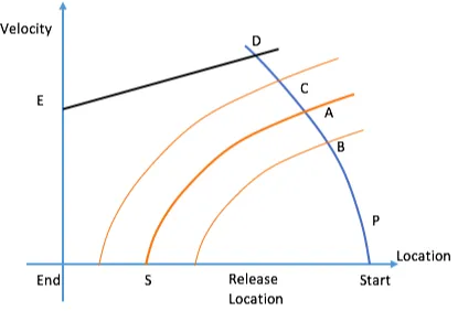
FIGURE 9: Safety warning information, schematic diagram.

For example, Figure 9 shows a location-velocity coordinate system. On this plane,

the blue curve P represents the behaviour of the test train when it is propelled by the propulsion cart. The black line DE is the coast-down phase of the test train. The other three orange curves with similar shape describe the brake behaviour of the

test train decelerated with the propulsion cart. The collision test starts at the Start

the test needs to be aborted, after the brake phase, the test train and propulsion cart

should finally stop between S and point Start in order to be safe. Otherwise, they will be too close to the barrier and may not stop safely. Point A is the last chance to abort a test. If the test is aborted at this point, the test train and propulsion cart

will just stop at pointS. Thus, when the test is aborted before pointA, such as point

B, the test train and propulsion cart can stop safely. However, if pointA is unknown and the test is still aborted at pointC, the test train and the propulsion cart will not be safe.

2

Deviation of Simulated Release Point from Real

Release Point

The RTPSA method could calculate precisely the release velocity and location in

simulation. Once the release velocity is reached, the train is right away released in

simulation. The simulation also demonstrates that the train will then hit the barrier

at the exact desired crash velocity. This positive result proves in principle that the

idea behind the RTPSA method works as expected, at least in simulation.

However, the inaccuracy occurs in simulating the last propulsion phase(mentioned

in chapter 2) with simple linear model introduced in the control/release module of

RTPSA. The motion of the test train in the last propulsion phase should be described

by a curve on a velocity-location coordinate system. However, this motion is simply

simulated by a straight line in the control/release module, which is an inaccurate

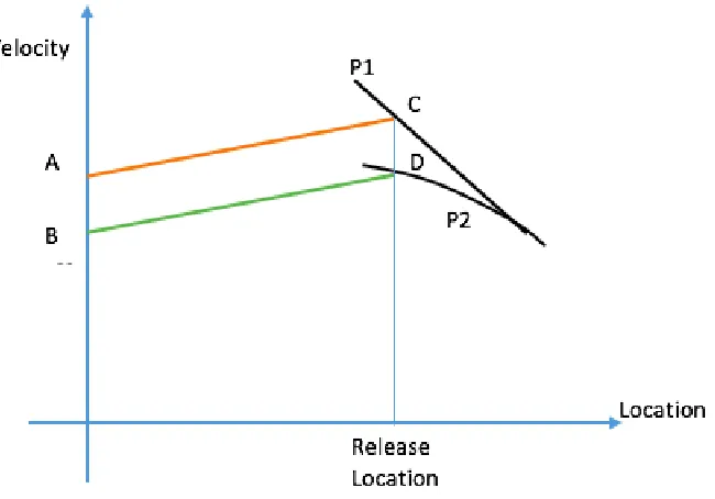
simulation. This inaccuracy has influence on releasing precisely. Figure 10 shows the

deviation of simulated release point from real release point. The X-axis is location,

FIGURE 10: Deviation of simulated release point from real release point, schematic

diagram.

real release point will be point D. As a result, the orange line AC represents the coast-down phase of the test train calculated by RTPSA, and the green line BD

describes the coast-down phase in a real test. Point A is the required crash point, and pointB is the real crash point. Obviously, there is deviation of real release point from caculated release point. This deviation will finally result in the inaccurate crash

velocity.

However, if the train can maintain the release velocity for a short time before

release(in other words, do uniform motion), it is easier to release the train and the

deviation of real release point and calculated release point can be minimized. As

shown in Figure 11, after accelerated by the propulsion cart, the test train will do

uniform motion before release. After this motion, the test train will coast down and

crash into the barrier with the desired velocity.

chap-FIGURE 11: The behaviour of the test train in improved RTPSA, schematic diagram.

ter. And in the next chapter, the proposed method, improved RTPSA, is introduced

Improved RTPSA

In order to solve the problem raised in the previous chapter, a new safety warning

module is combined with the original RTPSA. Moreover, the test train will move with

a uniform velocity before release, and the PID controller module is implemented to

monitor and control this uniform motion phase in order to minimize the deviation

between real release point and calculated release point. This chapter discusses the

design principle, software structure and the details of these two new modules.

1

Design Principles

1.1

Necessary Simulation Before Real Test

Improved RTPSA will be deployed in real time collision test, where the test train

will connect with the propulsion cart and be accelerated to a calculated release

ve-locity, and then, instead of being released right away at this veve-locity, the train will

move with this release velocity for a while and then disconnect with the propulsion

cart at a calculated release location, in order to minimize the deviation of real release

point from calculated( or called predicted) release point. Compared with the original

RTPSA, there are two new modules, safety warning module and PID controller

mod-ule, in improved RTPSA. In these two modules, there are some important parameters

which consists of the outputs of early safety warning module and the coefficients of

the PID controller. However, these important parameters are required to be decided

The outputs of early safety warning module is a set of early safety warning

in-formation. The early safety warning information includes two parts which are LCA

and LCR mentioned in chapter 3. It may not be proper if the safety warning infor-mation is calculated during the real test. Assuming the train is running and RTPSA

is calculating where is the release velocity/location and where is the last chance to

abort the test. However, this last chance may have already been missed during the

calculation before the result comes out. Then, even if the train is decelerated

imme-diately, the test still can not be aborted safely. This kind of situation occurs when

the length of the rail is too short or the propulsion force is too strong. To circumvent

this circumstance, the safety warning information should be obtained in a simulation

before the real test by studying simulated data.

FIGURE 12: Effect of proportional gain, schematic diagram[5].

The PID controller will detect and adjust the velocity during the uniform

mo-tion. As introduced in chapter 2 section 3, there are three important coefficients

KP, KI, KD, affecting the performance of the PID controller system. In Figure 12, the X-axis represents the time, while Y-axis is the status of the object controlled

by PID. The blue curve with two right angles indicates the ideal performance of the

The differentK in the right-top corner represents the different value of proportional gain KP, while KI and KD are fixed in this case. The performances of the object varying on different K is showed by different coloured curves. Moreover, the settling time is how much time the PID controller takes to adjust the object from one initial

status to an stable status. And the stability represents how smooth the performance

is. Obviously, in this figure, the stability and the settling time are significantly

influ-enced by the proportional gain. Although this figure only shows the effect ofKP, the other two coefficientsKI and KD also affect the performance of the controlled object. Moreover, these three coefficients are required to be tuned based on the performance

of the controller, and can not be simply calculated by any expression. Different PID

system may have different values of the coefficients to achieve expected performance,

such as expected settling time and stability. Even for the same system but different

setvalues, the best fitting coefficients might be different.

Generally, there are two ways to tune the coefficients. One is self-learning method[11]

in which the system implemented with a machine learning method can adjust the

co-efficients of PID controller itself by studying the performance of the controlled system.

This first way does not need human intervention and is normally used in the situation

when the requirement of the system(setpoint) always changes or is not predefined.

However, the machine learning process takes normally long time that cannot be

tol-erated in real time applications, thus is not selected in this project. In the second

way, the three coefficients of PID are tuned by the people with their experience or

software tools before PID controller is deployed. The drawback of the second way

is it always requires a person to update the PID coefficients when the requirement

varies. In this project the uniform motion velocity, which is also the setvalue of PID

controller, is not predefined before RTPSA is deployed. But time is precious in a real

time system, the first way is not proper in this project. As a result, the coefficients

1.2

Feasibility of the Calculation Based on Simulated Data

As introduced, some parameters of the safety warning module and PID controller

module is required to be calculated in a simulation test with simulated data. This

subsection will discusses the feasibility of this calculation which is based on simulated

data, in order to make sure if they are feasible in a real test.

The main drawback of the simulated data of a collision test is that the resistance

force(all the resistance mentioned in below only consists friction and aerodynamic

re-sistance) cannot be predicted precisely. Apart from the resistance, the other data(such

as propulsion force, brake force and so on) of a real test can be simulated with very

small deviation.

The purpose of the safety warning module is obtainingLCAandLCR(mentioned in chapter 3). The correctness of LCAand LCR is the most important requirement. If the test is aborted at or before LCA, the test train and the propulsion cart must definitely stop safely. However, as introducted, LCA and LCR are all calculated based on simulated data where the resistance can not be simulated precisely. If the

inaccurate resistance is still considered, the correctness of LCA and LCR cannot be guaranteed. However, as a conservative strategy, if the resistance is not considered

when calculating LCA and LCR, the test train must travel less distance in a real test where resistance exists, which can make sure the test train and propulsion cart

stop within the safety distance. The feasibility and details of this strategy will be

explained in the section “Early Safety Warning Module”.

In terms of the PID controller module, as introduced in chapter 2, it will control

the system to be dynamically equilibrium at the setvalue. In other words, the status

of the system will be controlled within a certain range, but not definitely just stay

coefficients can be found to satisfy a certain system, and at the same time one certain

set of PID coefficients may be qualified in different systems, as long as the status of

the systems are limited within an expected range. Thus, although the simulated data

may be different from the real test data, the PID coefficientsKp,Ki, andKdtuned in a simulation test can still be theoratically qualified in the corresponded real test. The

experiment results is satisfied as well. However, more experiments, especially real test

experiments, are still required in the future, since the current experiments are still

based on simulated data introduced in chapter 2 section 2. Although this simulated

data have already considered the deviation of real tests from simulations and try to

eliminate this deviation with compensatory values[18], it is still a compromise to test

the result of real data based on simulated data.

2

Software Structure

The original RPTSA is implemented and generates result as expected, however

there are still limitations which are discussed in chapter 3. The improved RTPSA

does not modify the original RTPSA but adding modules on it in order to obtain a

better result. Improved RTPSA has three parts, early safety warning module, original

RTPSA, and PID Controller Module.

FIGURE 13: Structure of original RTPSA[18].

The structure of the existing RTPSA is shown in Figure 13. The input of original

sensors in real test and is historicaland theoretical data in simulation tests which is

introduced in chapter 2 section 2. This data stream comes from the propulsion

sys-tem on the right side of the figure, and then feeds into coefficients calulation module

through the interface. The output coming from control/release module consists of two

parts. One of them is the release point consisting of the release velocity and location.

The other one is a demonstration video to demonstrate the whole test process. As

shown in this figure, RTPSA collects the data stream of the propulsion phase from

the hardware as the input of the coefficient calculation module. After calculation,

a set of coefficients b0, b1, b2(mentioned in chapter 2) indicating the relation between

resistance and velocity will be saved and passed to the coast-down simulation module

as the input. Based on this relation, the resistance of the coast-down motion can be

calculated and thus the whole performance of the coast-down phase can be predicted

bySETBDintroduced in chapter 2. Then, the stored coefficients will feed into propul-sion simulation module and another set of points SETCB(introduced in chapter 2) are generated to predict the last propulsion phase before release. Eventually, this two

sets of points will be treated as the input of the control/release module. The simple

linear regression model is applied to build the math models of coast-down phase and

propulsion phase. Then their intersection points is calculated and regarded as the

output - release velocity/location. This information will be sent back to the

hard-ware(FCS is short for facility control system) to physically release the test train.

In the improved RTPSA, two new modules, safety warning module and PID

con-troller module, are augmented to the previous system as shown in Figure 14.

The early safety warning module is firstly implemented. In this module, the early

safety warning information includingLCA and LCR is calculated before a real test. Then, this information will feed into the original RTPSA.

After safety warning information is transferred, the original RTPSA will still

op-erate in the almost same way as described in Figure 13. However, the only difference

occurs in the last step - control/release module. The release velocity and location

will be re-calculated. The details of the calculation will be discussed in the following

sections. Then, the new release velocity is transferred to PID controller module as

the setvalue to control the release process. When the test train reaches the release

velocity, PID controller will communicate with propulsion system to force the test

train to do uniform motion until it reaches the release location. After that, the test

train will be disconnected from propulsion system, and then hit the barrier with the

desired crash velocity.

3

Early Safety Warning Module

The early safety warning module focuses on two parts. The first part is the last

chance to abort the test train(LCA), when test train connects with propulsion system. The second part is the last chance to release the test train(LCR) in order to keep the propulsion cart safe.

3.1

Principle and Design

In this module,LCAandLCRwill be calculated. More specificly,LCAandLCR

will be represented by two certain locations called safety locations. In other words,

in terms of LCA, the test should be aborted before a safety location, and for LCR

In terms of LCA, the train is connected with propulsion cart. In this situation, firstly, the test train will be propelled by the propulsion cart to a safety location.

This process is called propulsion stage. Then the test train and propulsion cart is

decelerated to velocity zero and stops at or before the safety distance which is the

last location for the test train and the propulsion cart to stop safely. This process is

brake stage.

FIGURE 15: Parameters in LCA, schematic diagram.

As introduced, LCA will be calculated in a simulation before a real test is de-ployed. The resistance can not be simulated the same as the one in a real test.

calculating LCA(and LCR). The LCA calculated by this strategy may not be the best solution but will be completely correct.

Figure 15 shows the performance of the test train aboutLCAin a location-velocity coordinate system. The test train is propelled by the propulsion cart from the point

Start, and the barrier is located at the point End. The distance between End and

S is the safety distance introduced in chapter 3. The location of pointStart is zero. Assume that FP is the propulsion force in both of simulation and real test,FB is the brake force in both of simulation and real tests,m is the mass of propulsion cart and test train, R is the resistance force in real test. Lsl is the safety location of LCA calculated without resistance. If resistance is not in consideration, when the test is

aborted at Lsl the test train and the propulsion cart will finally stop completely at point S just as shown in Figure 15. On the other hand, in a real test,if the test is aborted at Lsl as well, the test train and the propulsion cart will finally stop at loca-tionLstop. Because of the influence of the resistance, Lstopmust be smaller thanS. As a result, the LCA calculated without R can guarantee the test train and propulsion cart stop safely.

So far, the correctness of Lsl is explained. In other words, if the test train and propulsion cart start to decelerate at or before Lsl, they will never reach S, thus can stop safely. Then the next goal is calculating where is Lsl.

As illustrated, the safety locationLsl should be calculated in the simulation with-out considering resistance. By observing Figure 15, Lsl is the intersection of the propulsion stage withoutR and the brake stage without R. The brake stage without

R can be described by the following equation,

−FB =m∗as2 (1)

where as2 is deceleration, FB >0. Thus as2 is calculated,

as2 = −FB

And the relation between location and velocity is shown by the following equations,

L=L0+

1 2as2t

2 ₍₃₎

v =v0+as2t (4)

where t is time, L is the location corresponded to the time,v0 and L0 are initial

velocity and intial location, and v is velocity. As the brake stage without R goes through the point where velocity is 0 and location is S, then, if the brake stage is calculated backwards from this point, v0 equals to 0 and L0 equals S. By solving the

equations (3) and (4), the relation between location and velocity can be calculated,

v =p2(L−S)as2 (5)

whereas2 is given by equation (2). LocationS, mass and brake forceFB are provided before a test. Based on these information, the value of as2 can be calculated.

In a similar way, the relation between location and velocity during the propulsion

stage withoutRcan also be calculated. The force of propulsion stage can be described by the following equation,

FP =m∗as1 (6)

where as1 is the acceleration. As the propulsion stage without R goes through the

Startpoint where location and velocity are both 0, the relation betweenv andL can be described,

v =p2Las1 (7)

where the value of as1 is obtained based on equation (6) and the information of mass

and propulsion force are provided as well.

The location of the solution of equation (5) and equation (7) is the safety location

Lsl. By solving these two equations,

Lsl =L=

as2+S

as2−as1

where as2, S, and as1 are known, thus Lsl can be calculated.

FIGURE 16: Same image as Figure 15.

So far, the calculation completes, if the train is propelled to a certain release

velocity and is released without doing any uniform motion. However, if there is an

uniform motion when the test train is propelled, the behaviour of the test train will

differ from the one without uniform motion. In Figure 16, the yellow line represents

the behaviour of uniform motion, where vunif orm is the velocity of uniform motion. So the test train and propulsion cart will first move as described by the propulsion

curve and then follow the uniform motion line, instead of moving on the propulsion

curve throughout. In this situation, if vs1 is the corresponding velocity of Lsl while resistance is not considered, then vs1 > vunif orm. By observing Figure 16, when

Lnsl is calculated by solving the equations (5) where v =vunif orm ,

Lnsl =L=

v2

unif orm 2as2

+S

. Thus, when vs1 < vunif orm, the value of Lsl is the safety location for LCA. On the other hand, while vs1 > vunif orm, the safety location is Lnsl. However, without the knowledge of vunif orm, it is impossible to determine which one is the safety location. Thus, the next goal is determining the value of vunif orm.

In terms of LCR, the safety location Lrsl for release will be calculated. Together with the safety location, the corresponding velocity vrsv is also calculated. If the propulsion cart releases the test train at or greater than vrsv and decelerates imme-diately, the propulsion cart can stop safely. In improved RTPSA, as the test train

will do uniform motion before being released, the release veloctiy just equals to the

velocity of uniform motion. Thus, the velocity of uniform motionvunif orm must equal to or be greater than the safety velocity vrsv. The goal of LCR is determining a proper velocity for the uniform motion in order to keep the propulsion cart safe after

release.

The configurations of the test in Figure 17 are same as Figure 15. But in this figure,

the test train will first be propelled to the velocity vunif orm, and do uniform motion with this velocity. The test train will be released at location Lrsl, and coast down to the barrier. Meanwhile, the propulsion cart(short for PC cart) will immediately

decelerate after release. Moreover, the location of point Start is zero as well in this figure.

FIGURE 17: Parameters in the second part of early safety warning module, schematic

release at Lrsl.

As vunif orm will not be affected by the resistance and vunif orm equals tovrsl when calculating LCR, Lrsl and vrsl will be same in both of the real test and the situa-tion without resistance. In other words, in both situasitua-tions, the propulsion cart will

release the test train at the same location and velocity. Because of the resistance,

the inequalityLrstop < S is gained. In other words, althoughLrsl is obtained without considering the resistance, if the test train is released atvrsl in a real test, the propul-sion cart can still stop safely. Then, next goal is to calculate the value ofvrsv andLrsl.

The brake stage of propulsion cart for LCR starts from the time when test train is just released, and ends at the time when the propulsion cart completely stops. The

relation between location L and velocity v of the brake stage of propulsion cart can be described by the following equation,

v =p2(L−S)ar (9)

wherearis the deceleration of the propulsion cart, and can be defined by the following equation,

ar =

−FB

mpc

whereFB is the brake force, andmpc is the mass of the propulsion cart. And all these information can be obtained before simulation.

In improved RTPSA, the release location/velocity is the intersection of uniform

motion and coast-down motion. The safety location of LCR - the last chance to release the propulsion cart - is also one of the possible release locotions. Thus, location

Lrsl and velocityvrsv must be on the coast-down phase. In other words, this location and velocity is the intersection of the brake stage of propulsion cart and coast-down

phase. In order to obtain the coast-down phase, RTPSA is required to be applied

then, the coast-down phase is calculated and described by the following equtaion,

v =aL+b (10)

where coefficientsaandb are calculated by RTPSA. By sovling the equations (9) and (10), the values ofLrsl and vrsv are obtained.

As shown in Figure 17, the brake stage of the propulsion cart is almost vertical to

the location-axis, reflecting that the brake time of the propulsion cart is short, since

the mass of propulsion cart is small while the brake force is huge. Apart from extreme

cases( such as the rail is too short or the crash velocity is too large), the propulsion

cart is generally safe in the original RTPSA where the uniform motion is excluded,

because the time for the coast-down phase is way greater than the time for the brake

stage of propulsion cart. However, after uniform motion is included, the time of the

coast-down process is critically cut down. As shown in Figure 18, assuming segment

HI indicates the uniform motion, the test train will be detached at pointI instead of the original release pointB, which leads to the significant reduction of the coast-down phase, from BD to ID. If point J represents the intersection of the brake stage of propulsion cart and coast-down phase, the propulsion cart is dangerous after release

when the velocity of pointI is smaller than the velocity of point J. In order to avoid this situation, the velocity for the uniform motion vunif orm should be greater than the velocity of point J which is the safety velocity vrsv. And vunif orm should also be smaller than the velocity of point B. As a result, the velocity of the uniform motion is calculated as following,

vunif orm =b

vrsv +vorv

2 c

where vorv is the orignal release velocity calculated by RTPSA which is also the ve-locity of point B.

Moreover, the uniform motion velocity is also the release velocity. And the release

velocity and location must be on the coast-down phase. In a real test, improved

but with different value ofaandb. By solving this equation with the value ofvunif orm, the new release location is obtained.

FIGURE 18: Uniform motion in original RTPSA, schematic diagram.

3.2

Program Logic

In Figure 19, the flow chart for the early safety warning module describes the

program logic in the improved RTPSA.

First, the data stream, consisting of the mass, force, safety distance and other basic

information, is transferred to this module. And then, the math models indicating each

phase of motion are built. One of them, the model for brake stage of propulsion cart

is prepared to feed into RTPSA for simulation. In terms of other two models, the

propulsion phase for the test cart and the propulsion cart and the brake process of

these two objects, the location of their intersection will be regarded as the initial

version of the last chance to abort a test. Both of this safety location and the math

model of the brake phase for the two objects will be collected by the RTPSA as well.