University of Windsor University of Windsor
Scholarship at UWindsor
Scholarship at UWindsor
Electronic Theses and Dissertations Theses, Dissertations, and Major Papers
9-17-2018
Parameterization Of The Exhaust-Fascia Interface Using
Parameterization Of The Exhaust-Fascia Interface Using
Surrogate Modelling
Surrogate Modelling
Tyler Doyle
University of Windsor
Follow this and additional works at: https://scholar.uwindsor.ca/etd
Recommended Citation Recommended Citation
Doyle, Tyler, "Parameterization Of The Exhaust-Fascia Interface Using Surrogate Modelling" (2018). Electronic Theses and Dissertations. 7515.
https://scholar.uwindsor.ca/etd/7515
This online database contains the full-text of PhD dissertations and Masters’ theses of University of Windsor students from 1954 forward. These documents are made available for personal study and research purposes only, in accordance with the Canadian Copyright Act and the Creative Commons license—CC BY-NC-ND (Attribution, Non-Commercial, No Derivative Works). Under this license, works must always be attributed to the copyright holder (original author), cannot be used for any commercial purposes, and may not be altered. Any other use would require the permission of the copyright holder. Students may inquire about withdrawing their dissertation and/or thesis from this database. For additional inquiries, please contact the repository administrator via email
Parameterization Of The Exhaust-Fascia Interface
Using Surrogate Modelling
by
Tyler Doyle
A Thesis
Submitted to the Faculty of Graduate Studies
through the Department of Mechanical, Automotive & Materials Engineering in Partial Fulllment of the Requirements for
the Degree of Master of Applied Science at the University of Windsor
Windsor, Ontario, Canada
2018
Parameterization Of The Exhaust-Fascia Interface
Using Surrogate Modelling
by
Tyler Doyle
APPROVED BY:
P. Henshaw
Department of Civil & Environmental Engineering
V. Roussinova
Department of Mechanical, Automotive & Materials Engineering
J. Defoe, Advisor
Department of Mechanical, Automotive & Materials Engineering
Author's Declaration of Originality
I hereby certify that I am the sole author of this thesis and that no part of this thesis has been published or submitted for publication.
Abstract
Currently, full vehicle computational uid dynamics (CFD) simulations are used to predict rear fascia temperatures. As these simulations are expensive and time consuming, only what is intended to be a worst case scenario analysis is completed. Certain variables can be overlooked and the case selected may not be the worst case scenario. The objective of this thesis is to create a surrogate model that can rapidly predict maximum fascia temperature for a variety of vehicle operating conditions and exhaust positions, while exploring the physical mechanisms responsible for the heat transfer between the exhaust gas, exhaust components, and rear fascia.
Using full vehicle CFD simulations, an investigation of the maximum fascia tem-perature as a function of vehicle operating conditions and exhaust positioning is com-pleted by identifying non-dimensional parameters governing maximum fascia temper-ature, consisting of both geometric and non-geometric parameters based on vehicle speed and exhaust inlet velocity (Reynolds number), their ratio (velocity ratio), and exhaust temperature (exhaust temperature ratio). The exhaust positioning within the rear fascia is simplied into four non-dimensional parameters to explore the mod-ications in geometry.
Acknowledgments
Completing a thesis while spending a year abroad has not been an easy feat and I thank those around me for their condence and motivation throughout the last two years.
My supervisor, Dr. Defoe, thank you for all your assistance throughout my the-sis. Your commitment to research and education, as well as your simple approach to problem solving is something I will continue to carry with me throughout my career. Thank you to everyone at Fiat Chrysler Canada Automotive Research and Devel-opment Centre (ARDC), Chrysler Technical Center (CTC), Centro Richerche Fiat (CRF) who I have met with and have been there to answer any questions throughout my research. My industrial supervisor, Erin Farbar, thank you for always being there to answer my questions and work through any diculties.
Thank you to Dr. Johrendt at the University of Windsor and Dr. Belingardi at Politecnico di Torino for all the work you've done to help make the International Master's program an incredible experience.
Thank you to my committee members Dr. Henshaw and Dr. Roussinova for taking the time to review my thesis and provide feedback throughout my research.
Contents
Author's Declaration of Originality iii
Abstract iv
Acknowledgments v
List of Figures ix
List of Tables xvi
Nomenclature xvii
1 Introduction 1
1.1 Objectives . . . 4 1.2 Key Outcomes . . . 4 1.3 High Level Outline . . . 6
2 Literature Review 7
2.1 Heat Transfer Modelling and CFD Best Practices . . . 8 2.2 Key Vehicle Thermal Management Case . . . 12 2.3 Surrogate Model Construction . . . 13
3 Approach 19
3.2 CFD Simulations . . . 24
3.3 Parameter Development . . . 34
3.3.1 Geometric Parameter Development . . . 34
3.3.2 Non-Geometric Parameter Development . . . 36
3.3.2.1 Non-Geometric Parameter Design Space . . . 39
3.4 Design of Experiments . . . 42
3.5 Surrogate Model Generation . . . 43
4 Results 44 4.1 Assessment of CFD Results . . . 44
4.2 Model Construction . . . 47
4.3 Model Assessment . . . 47
4.3.1 Model Prediction Error . . . 47
4.3.2 Geometric Parameters . . . 49
4.3.2.1 X+ . . . 50
4.3.2.2 Y+ . . . 56
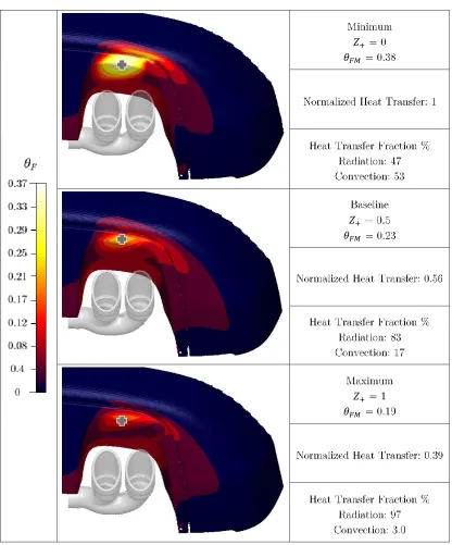
4.3.2.3 Z+ . . . 61
4.3.2.4 β+ . . . 65
4.3.3 Non-Geometric Parameters . . . 70
4.3.3.1 Exhaust Temperature . . . 71
4.3.3.2 Vehicle Speed and Exhaust Velocity . . . 73
4.3.3.3 R=0 . . . 75
4.3.3.4 R>0 . . . 79
4.3.4 Final Surrogate Model Predictions (SM2) . . . 88
4.3.4.1 Non-Geometric . . . 88
5 Summary, Conclusions, and Recommendations for Future Work 91
5.1 Summary . . . 91
5.2 Conclusions . . . 93
5.2.1 Contributions . . . 94
5.3 Future Work . . . 96
5.3.1 Location Analysis . . . 96
5.3.2 Exhaust Geometry . . . 96
5.3.3 Velocity Measurements for Reynolds Number Calculations . . 97
5.3.4 Improvements to CFD Modelling . . . 98
Bibliography 100 A DOE Samples 103 B Calculations 104 B.0.1 Mach Number Calculation . . . 104
B.0.2 Reynolds Number Calculation - Constant Properties - 311 K, UJ=83.68 . . . 104
B.0.3 Reynolds Number Calculation - Variable Properties - 1242 K, UJ=83.68 . . . 105
C EBF Model Matrices 106 C.0.1 Initial Model -SM1- Inputs: 7, Outputs: 1, Designs: 24 . . . 106
C.0.2 Final Model - SM2- Inputs: 7, Outputs: 1, Designs: 43 . . . . 108
List of Figures
1-1 Comparison of traditional and modern exhaust packaging. Left:
tra-ditional; right: modern. . . 2
1-2 Convection and radiation govern the heat transfer to and from the fascia. . . 3
2-1 A 2 input, 10 level full factorial sample. . . 14
2-2 Sampling on a 2 input, 10-point LHS. [17] . . . 14
2-3 Sampling on a 2 input, 10-point OLHS. [17] . . . 16
3-1 Flowchart of approach taken to complete the research. . . 20
3-2 Top: coherent exhaust jet; bottom: non-coherent exhaust jet. . . 23
3-3 C-SUV used for all CFD simulations. . . 24
3-4 CFD domain matches experimental conguration. . . 26
3-5 Heat transfer resistance diagram, to and from the fascia. Dashed: radiative; solid: convective. . . 27
3-6 Uniform velocity inlet simulates exhaust ow. . . 29
3-7 Flow separation in center section of the exhaust tailpipe, from CFD data. Viewing XY plane. . . 30
3-8 Trailer used in CFD simulations and its dimensions. . . 31
3-10 Decrease in under-body convective velocity in large domain. Velocity contours cut at centre of vehicle. Left: small domain; right: large
domain. . . 33
3-11 Chain of dependency between experimental data and conguration used for surrogate model. . . 33
3-12 Geometric parameters (driver's side view forX+ andβ+ and rear view for Y+ and Z+). . . 35
3-13 Modifying β+ while maintaining X+ and Z+. . . 37
3-14 θF M∗ values of cases simulated with CFD to determine non-geometric parameters. . . 39
3-15 Engine map of exhaust conditions at the catalytic converter. . . 40
3-16 GT-Power model sets CFD boundary conditions. . . 41
3-17 Exhaust conditions at CFD exhaust jet inlet, extracted from GT-Power. 42 4-1 Thermocouple locations do not capture hotspot location. . . 45
4-2 DOE Results. . . 47
4-3 Fascia area used for heat transfer analysis. . . 49
4-4 Predicted vs. CFD θF M values for X+. . . 50
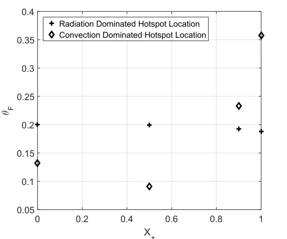
4-5 Heat transfer and θF values for X+. θF M located with gray cross. . . 52
4-6 Exhaust jet and fascia θF contours for X+= 0. Top: view towards inboard exhaust tip, plane cut at centre of inboard exhaust tip; bottom: view towards outboard exhaust tip, plane cut at centre of outboard exhaust tip. Exhaust, as well as fascia surface behind plane do not haveθF contours. . . 53
4-8 Exhaust jet and fascia θF contours for X+ = 0.9. Top: view towards
inboard exhaust tip, plane cut at centre of inboard exhaust tip; bottom: view towards outboard exhaust tip, plane cut at centre of outboard
exhaust tip. . . 54
4-9 Exhaust jet and fascia θF contours for X+ = 1. Top: view towards inboard exhaust tip, plane cut at centre of inboard exhaust tip; bottom: view towards outboard exhaust tip, plane cut at centre of outboard exhaust tip. . . 54
4-10 θF values for X+ at the two locations of θF M, CFD results. . . 56
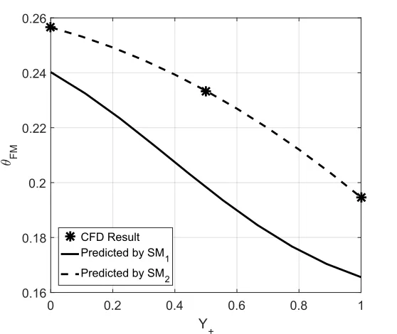
4-11 Predicted vs. CFD θF M values for Y+. . . 57
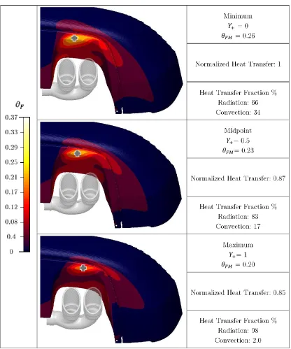
4-12 Heat transfer and θF values for Y+. . . 58
4-13 Exhaust jet and fascia θF contours for Y+ = 0. Top: view towards inboard exhaust tip, plane cut at centre of inboard exhaust tip; bottom: view towards outboard exhaust tip, plane cut at centre of outboard exhaust tip. . . 59
4-14 Exhaust jet and fascia θF contours for Y+ = 0.5. Top: view towards inboard exhaust tip, plane cut at centre of inboard exhaust tip; bottom: view towards outboard exhaust tip; plane cut at centre of outboard exhaust tip. . . 59
4-15 Exhaust jet and fascia θF contours for Y+ = 0.5. Top: view towards inboard exhaust tip, plane cut at centre of inboard exhaust tip; bottom: view towards outboard exhaust tip, plane cut at centre of outboard exhaust tip. . . 60
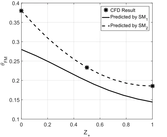
4-16 Predicted vs. CFD θF M values for Z+. . . 61
4-18 Exhaust jet and fascia θF contours for Z+ = 0. Top: view towards
inboard exhaust tip, plane cut at centre of inboard exhaust tip; bottom: view towards outboard exhaust tip, plane cut at centre of outboard exhaust tip. . . 63 4-19 Exhaust jet and fascia θF contours for Z+ = 0.5. Top: view towards
inboard exhaust tip, plane cut at centre of inboard exhaust tip; bottom: view towards outboard exhaust tip, plane cut at centre of outboard exhaust tip. . . 64 4-20 Exhaust jet and fascia θF contours for Z+ = 1. Top: view towards
inboard exhaust tip, plane cut at centre of inboard exhaust tip; bottom: view towards outboard exhaust tip, plane cut at centre of outboard exhaust tip. . . 64 4-21 Predicted vs. CFD θF M values for β+. . . 65
4-22 Heat transfer and θF values for β+. . . 66
4-23 Exhaust jet and fascia θF contours for β+ = 0. Top: view towards
inboard exhaust tip, plane cut at centre of inboard exhaust tip; bottom: view towards outboard exhaust tip, plane cut at centre of outboard exhaust tip. . . 67 4-24 Exhaust jet and fascia θF contours for β+ = 0.21. Top: view towards
inboard exhaust tip, plane cut at centre of inboard exhaust tip; bottom: view towards outboard exhaust tip, plane cut at centre of outboard exhaust tip. . . 67 4-25 Exhaust jet and fascia θF contours for β+ = 0.5. Top: view towards
4-26 Exhaust jet and fascia θF contours for β+ = 1. Top: view towards
inboard exhaust tip, plane cut at centre of inboard exhaust tip; bottom: view towards outboard exhaust tip, plane cut at centre of outboard
exhaust tip. . . 69
4-27 θF M prediction with increasing β+ values at aReV value of 0. . . 70
4-28 ETR4 cases studied, shown on the engine map. . . 72
4-29 Predicted vs. CFD θF M values for ETR4. . . 73
4-30 Predicted vs. CFD θF M values for increasing ReV with increasing ReJ. 75 4-31 Heat transfer and θF values for R= 0, increasing ReJ. . . 77
4-32 Exhaust jet and fascia θF contours for R = 0, ReJ = 1.23× 10⁵. Top: view towards inboard exhaust tip, plane cut at centre of inboard exhaust tip; bottom: view towards outboard exhaust tip, plane cut at centre of outboard exhaust tip. . . 78
4-33 Exhaust jet and fascia θF contours for R = 0, ReJ = 3.66× 10⁵. Top: view towards inboard exhaust tip, plane cut at centre of inboard exhaust tip; bottom: view towards outboard exhaust tip, plane cut at centre of outboard exhaust tip. . . 78
4-34 Exhaust jet and fascia θF contours for R = 0, ReJ = 6.06× 10⁵. Top: view towards inboard exhaust tip, plane cut at centre of inboard exhaust tip; bottom: view towards outboard exhaust tip, plane cut at centre of outboard exhaust tip. . . 79
4-35 θF M values for R >0 and ET R4 = 88.3. . . 80
4-36 Heat transfer and θF values for non-zero R values, increasing R. . . . 82
4-38 Exhaust jet and fascia θF contours for R = 0.20. Top: view towards inboard exhaust tip, plane cut at centre of inboard exhaust tip; bottom: view towards outboard exhaust tip, plane cut at centre of outboard exhaust tip. . . 83 4-39 Exhaust jet and fascia θF contours for R = 0.24. Top: view towards
inboard exhaust tip, plane cut at centre of inboard exhaust tip; bottom: view towards outboard exhaust tip, plane cut at centre of outboard exhaust tip. . . 84 4-40 Exhaust jet and fascia θF contours for R = 0.39. Top: view towards
inboard exhaust tip, plane cut at centre of inboard exhaust tip; bottom: view towards outboard exhaust tip, plane cut at centre of outboard exhaust tip. . . 84 4-41 Exhaust jet and fascia θF contours for R = 0.58. Top: view towards
inboard exhaust tip, plane cut at centre of inboard exhaust tip; bottom: view towards outboard exhaust tip, plane cut at centre of outboard exhaust tip. . . 85 4-42 Exhaust jet and fascia velocity contours for R= 1.2. Exhaust outlined
in white. View towards inboard exhaust tip. Top: velocity plane cut at centre of inboard exhaust tip; bottom: plane cut at centre of outboard exhaust tip. . . 87 4-43 Exhaust jet and fascia θF contours for R = 1.2. Top: view towards
5-1 Exhaust jet and fascia velocity contours for R= 1.2. Exhaust outlined
List of Tables
3.1 Case used to assess grid independence. . . 30
3.2 Grid independence renement results. . . 31
3.3 Baseline (normalized) geometric values. . . 35
3.4 Cases analyzed to determine non-geometric parameters. . . 38
4.1 Boundary conditions for assessment of CFD. . . 44
4.2 Absolute dierence in θF and temperature between CFD and experi-mentally measured values. . . 46
4.3 Model assessment cases. . . 48
4.4 Cases analyzed for exhaust temperature. . . 72
4.5 Cases simulated with CFD for ReV and ReJ analysis. . . 74
4.6 ReV and ReJ values for R >0and ET R4 = 88.3. . . 80
4.7 Non-geometric parameters predicted bySM2to yield highest maximum fascia temperature. . . 88
4.8 Exhaust position predicted by SM2 to produce lowest maximum fascia temperatures. . . 89
Nomenclature
Symbols
β+ beta - exhaust rotation
D diameter d distance
ET R Exhaust temperature ratio f polynomial function
H vehicle height J index
k− K-epsilon λ design
L vehicle length
Φp optimality criterion
ϕbasis function R Reynolds ratio Re Reynolds number S covariance matrix SM surrogate model T temperature
υ kinematic viscosity W vehicle width ω weighting function x sample point
xc basis function centre
y unknown function of interest
X+, Y+, Z+ Exhaust translation directions
X, Y, Z cartesian coordinates
Subscripts
1, 2surrogate model 1 and 2
F fascia
F M fascia maximum i, j, k, m indices
∞ free stream
J jet
s number of distinct distance values in maximin criterion V vehicle
Superscripts
p positive integer
Abbreviations
CFD Computational Fluid Dynamics CRF Centro Richerche Fiat
CTC Chrysler Technical Center DOE Design of Experiments DOM Discrete Ordinate Method EBF Elliptical Basis Function FCA Fiat Chrysler Automobiles HPC High Performance Computing LHS Latin Hypercube Sampling NVH Noise Vibration Harshness
OLHS Optimal Latin Hypercube Sampling RANS Reynolds-Averaged Navier-Stokes RBF Radial Basis Function
RTE Radiative Transfer Equation S2S Surface to Surface
Chapter 1
Introduction
Automakers have, since the early 2000's, begun packaging the exhaust components within the rear bumper, also known as the rear fascia. These packing congurations, primarily motivated by aesthetics, also place the exhaust system closer to the under-body, reducing interaction with the under-body ow. Since it is not a structural component, the rear fascia is typically a plastic part to reduce weight. There are multiple packaging techniques used throughout the industry, but regardless of the technique, the hot exhaust components and exhaust gas are in close vicinity to the plastic fascia. An example of traditional and modern exhaust packaging is illustrated in Figure 1-1.
the heat transfer between the exhaust and fascia, the case that yields the highest fascia temperatures may be overlooked by such a selective approach, resulting in a maximum fascia temperature that is in excess of the maximum allowable value.
Figure 1-1: Comparison of traditional and modern exhaust packaging. Left: tradi-tional; right: modern.
While the simulations' accuracy is not always known, even measuring these tem-peratures experimentally is non-trivial. Typically measurements are completed with thermocouples; however, peak temperatures can be missed due to improper place-ment, as thermocouples essentially provide a point measurement. Eective use of both CFD and experiments together is important as, computations can more easily reveal trends and the expected locations of the maximum fascia temperature, while experimental tests yield reliable temperature values at the operating condition and location that is identied as the worst case.
ex-of running multiple CFD simulations for a specic design, a model generated from CFD simulations for a generic conguration will be able to quickly predict the maxi-mum fascia temperature for any load condition. Using experimental data to validate the model will ensure the predictions are reliable and can be used instead of lengthy design studies.
Thus, an approach that combines CFD, experiments to assess data, and surro-gate modelling is likely required to successfully predict maximum fascia temperatures during the design stage. When a design does have unacceptably high temperatures, insight into what governs the maximum fascia temperature can be used to generate a suitable alternative design.
Figure 1-2: Convection and radiation govern the heat transfer to and from the fascia.
heat transfer from the exhaust tips and convection from the exhaust jets. From the fascia, there is radiation heat transfer to the surroundings and convection to the under-body ow.
1.1 Objectives
The two main objectives of this thesis are to:
1. identify key parameters that characterize the uid-thermal interaction of the exhaust-fascia system and their various sensitivities and importance, and
2. use design of experiments (DOE) to develop a model that can predict maximum fascia temperatures for a variety of exhaust positions.
1.2 Key Outcomes
The key outcomes of this thesis are:
1. Two heat transfer mechanisms; radiation and convection govern the behavior of the heat transfer between the exhaust parts, exhaust gas, and rear fascia. Changing an operating condition or the positioning of the exhaust within the fascia will change the net amounts of radiative and convective heat transfer to the fascia. This will determine both the location and temperature of the hot-spot on the fascia.
2. The highest maximum fascia temperatures occur at a vehicle speed of zero. In-creasing vehicle speed lowers the maximum fascia temperature until a minimum is reached and then it increases again as vehicle speed increases.
maxi-speed will result in the highest fascia temperatures. This corresponds to wide open throttle (WOT) conditions while driving slowly. This could be during heavy towing conditions at very low speed. With a baseline geometry, the case predicted by the nal surrogate model to produce the highest fascia temperature exceeds the maximum allowable value by 200 K.
4. The nal surrogate model suggests that keeping the exhaust components as far away from the fascia as possible, decreasing its surface area, while aiming the exhaust downwards from the fascia will result in the lowest fascia tempera-tures. This decreases the two governing mechanisms: radiation and convection, and thus the total heat transfer to the fascia. In comparison to the baseline geometry, for the load condition resulting in the highest maximum fascia tem-perature, the optimal geometry is reduces the maximum fascia temperature so that it exceeds the allowable value by only 70 K.
5. The exhaust velocity's inuence on maximum fascia temperature is directly related to the vehicle speed and thus the ratio of the vehicle speed to the exhaust velocity. At a value of 0.24, the ratio was found to yield highest maximum fascia temperatures due to the exhaust jets' ability to remain coherent, while being directed towards the fascia by the under-body ow.
1.3 High Level Outline
Chapter 2
Literature Review
Little research in the open literature can be found related to heat transfer mechanisms governing temperatures for the exhaust jet and the surrounding area. Much of the existing work has focused on noise, vibration, and harshness (NVH) instead.
Research completed by Srinivasan et al. [1] and Eller et al. [2] has been done to ensure that high temperature components do not damage the parts around them. However, this was done for under-hood or under-body components and not the rear fascia area of the vehicle. For thermal protection of under-hood and under-body com-ponents, there is no exhaust jet; however, exhaust parts are modelled. Srinivasan et al. applied an isothermal boundary condition to model exhaust components, whereas Xiao et al. [3] applied a constant heat ux to the exhaust components. To best model the exhaust components in this thesis, these methodologies are reviewed in Section 2.1. Research of the heat transfer from high temperature jets to surrounding surfaces, such as that by Spring et al. [4] is used to better understand parameters involved in the heat transfer from the exhaust jet to the rear fascia. Furthermore, modelling techniques from these studies can be used to study the heat transfer between the exhaust and rear fascia, which is the focus of this thesis.
been proven to be eective and has been applied to many areas of research such as high speed civil transport, airfoil shape optimization, diuser shape optimization, and injectors [5].
2.1 Heat Transfer Modelling and CFD Best
Prac-tices
CFD simulations should be able to accurately capture the relevant physical mecha-nisms for both the ow and heat transfer. The main challenge in this is related to correctly predicting the Nusselt number. This is because it depends on the details of the turbulent momentum transport and so it is aected by the choice and accuracy of the turbulence model in Reynolds-averaged Navier-Stokes (RANS) computations. This is noted by Spring et al. [4] who investigated CFD-based prediction of heat transfer from a jet in a cross-ow. The authors note that the standard k−ε model
exhaust jet on the fascia), increasing the external ow velocity will produce higher heat transfer coecients and Nusselt numbers. This corresponds to increased vehicle speeds increasing the convective transport of the exhaust jet.
To non-dimensionally analyze a jet and external ow velocity, Spring et al. dened the Reynolds number of both the jet and external ow. They dened the jet Reynolds number with respect to the diameter of the jet inlet. In other research investigating jets in external ows, such as the work done by Jendoubi et al. [6], Michalke et al. [7], and Chan et al. [8], the authors dened a velocity ratio of U∞
UJ−U∞,
UJ−U∞ UJ+U∞, and UJ
U∞, respectively, where UJ and U∞ are the jet velocity and external ow velocity, respectively. For this thesis, the vehicle Reynolds number (ReV) is easily dened with respect to the vehicle speed (external ow velocity) and the vehicle length. The exhaust jet Reynolds number (ReJ), as dened by Spring et al., can be calculated with respect to the jet inlet diameter. The velocity ratio, R, can be dened as the
ratio between the vehicle and exhaust jet velocity, R= UV
UJ, avoiding division by zero at a vehicle speed of zero.
Srinivasan et al. [1] outline a procedure for vehicle thermal protection develop-ment that uses three-dimensional CFD to determine high temperature regions on the vehicle under-body. The procedure used a coupled convection-radiation simulation. It neglected conduction, as the conductivity of the most thermally sensitive compo-nents (elastomers, plastics, and rubbers) is poor. They were treated as adiabatic boundaries without signicant loss of accuracy. The computation was carried out using the commercial package CFD-ACE+ which is a general purpose unstructured control volume based Navier-Stokes ow solver. Standard k− turbulence model in
sys-tem. Through the use of this methodology, CFD temperatures and experimental test values were compared. For 13 components, it was found that on average, the CFD over predicted temperatures by 4 K with an average error of 8.29%. This could be attributed to the adiabatic boundary condition employed on the thermally sensitive parts. The procedure provided by Srinivasan et al. provides an accurate method to use for the exhaust part boundary conditions (isothermal), as well as the boundary conditions for the fascia (adiabatic).
Xiao et al. [3] also studied the radiation and conjugate heat transfer for the vehicle under-body. The authors completed a steady state analysis considering radiation and conjugate heat transfers. Unlike Srinivasan et al., they incorporated conduction into the analysis. They calculated the component temperature by integrating conjugate heat transfer on internal and external airow of the exhaust system. Star-CD was used which solves the RANS equation using a nite volume technique. The high-Reynolds number k − turbulence model was used. Conduction was solved for both uid
CFD computations does not consider cooling via the external air as done by Xiao et al. [3]; however, one-dimensional skin temperatures are computed with convection to the external air, decreasing potential error.
Zhang and Romzek [9] outline the use of CFD in vehicle exhaust systems. They noted that the majority mass fraction of exhaust gas is nitrogen, and experimental test results show the exhaust gas can be treated as ideal gas. This was also conrmed by Xiao et al. [3] who also assumed that the gas can be modelled as air and treated as an ideal gas. Zhang and Romzek also note that the uid ow inside the exhaust pipe is primarily turbulent ow and that thek−turbulence model can be used. For
exhaust boundary conditions, they found that commonly, inlet boundary conditions are exhaust gas mass ow rate and temperature. Lastly, they noted that emissivity of material is another critical input to accurately simulate skin temperature when a radiation heat transfer model is active. This was also mentioned in the procedure outlined by Srinivasan et al. [1].
Kandylas and Stamatelos [10] investigated exhaust system design based on heat transfer computation. In their work, it is stated that although the exhaust gas ow in a real exhaust system is unsteady and compressible, the variation of pressure in automotive exhaust systems is on the order of 0.01 kPa and thus is of negligible importance. For this narrow pressure range, density was determined to be a function of temperature, and thus the ow of exhaust gas could be assumed to be steady and incompressible. Their model showed good agreement between computational and experimental exhaust gas temperatures.
nitrogen is 3521 K, and exhaust gas temperatures are typically below 1300 K, one would not expect to see any signicant radiation heat transfer from the exhaust jets to the rear fascia.
In summary, both the vehicle (ReV) and jet (ReJ) Reynolds numbers non-dimensionalize the external and jet ow, respectively. A velocity ratio, R, the ratio between vehicle
and exhaust inlet velocity, where R = UV
UJ can be used to non-dimensionally analyze the two ows. The procedure described by Srinivasan et al. provided good agreement between experimental and CFD results while simplifying the heat transfer, removing conduction. Although it did not incorporate an exhaust jet, other studies indicate that it can be modelled as steady, incompressible and turbulent air. Modest indicates that neglecting radiation heat transfer from air is acceptable as the exhaust gas will not reach high enough temperatures to cause any signicant radiation heat transfer. This past work sets the stage to complete the problem of determining the maximum fascia temperature due to the heat transfer from exhaust parts and exhaust jets.
2.2 Key Vehicle Thermal Management Case
2.3 Surrogate Model Construction
The motivation for surrogate modelling is clearly dened in the literature. A sur-rogate approach saves time and money by decreasing the amount of experiments (whether physical or computational) completed, while allowing for fast analysis and approximations [12]. Similar denitions can be found in [5, 13, 14, 15, 16]. Surro-gate modelling methodology can be found in many papers [5, 13, 14, 15] and also in textbooks [12, 16]. The methodology is similar between each piece of literature; how-ever, the procedure outlined by Forrester et al. in Engineering Design via Surrogate Modelling [12], known as the surrogate modelling process was found to be the most clear and concise and is summarized below with additional information from other resources.
1. The design space is identied. The outputs of interest are identied and the inputs that impact the output(s) are analyzed. Here, the ranges of the input parameters can be selected as well.
2. Design of experiments (DOE) is completed. To generate the surrogate model, a sampling method is chosen to distribute the samples uniformly within the design space. A uniform level of model accuracy throughout the design space requires a uniform spread of points. When the number of input variables are small, or the experiments are not time consuming, full factorial sampling can be used [12]. Mckay et al. [13] notes that one of the most popular DOE methods for (relatively) uniform sample distributions is Latin hypercube sampling (LHS).
A full factorial sample uses every combination of inputs at the specied number of levels. As shown in Figure 2-1, 2 inputs with their range divided into 10 levels results in 100 experiments (102). The design space is uniformly sampled; however, many
single input sampled at the same 10 levels results in an increase of 900 experiments.
Figure 2-1: A 2 input, 10 level full factorial sample.
The LHS technique allows the designer total freedom in selecting the number of designs (λ) to run (as long as it is greater than the number of inputs), but at least3λ
designs is recommended to initialize a surrogate model [17]. LHS divides the design space into λ equal sized hypercubes known as bins. A point is placed randomly into
each bin ensuring that the design space can be exited along any direction parallel to any axis without encountering any of the other occupied bins. In Figure 2-2, a 2 input, ten-point (ten-design) LHS is shown. Each row and column only contain one point, but the points are not distributed evenly throughout the design space.
A drawback to LHS is that it is not reproducible because samples are generated with random combinations [17]. In addition, as the number of points decreases, the chances of missing some regions of the design space increases [17]. To uniformly distribute the points evenly throughout the design space, the optimal Latin hyper-cube sampling (OLHS) method was developed [17]. The OLHS method gives the best opportunity to model the true function of the response across the range of the inputs [12]. OLHS uses an optimality criterion known as the φp criterion, based on the maximin distance criterion [17], which ensures the points are uniformly spaced throughout the design space while following the LHS methodology.
The following OLHS process is described by [17, 18]. First, a normal LHS is run. The design is a maximin distance design, [19] if it maximizes the minimum inter-site distance:
min1≤i, j≤λ, i6=jd(xi, xj)
where d(xi, xj) is the distance between two sample points xi and xj:
d(xi, xj) =dij =
" m X
k=1
|xik−xjk|t
#1/t
, t = 1or2
Morris and Mitchell [20] built upon the maximin distance criterion. Further de-scribed by [17, 18], for a given design, by sorting all the inter-sited distance dij(1≤
i, j ≤ λ, i 6=j), a distance list (d1, d2, ..., ds), and an index list (J1, J2, . . . , Js) are obtained, where di's are distinct distance values with d1 < d2 < · · · < ds, Ji is the number of pairs of sites in the design separated bydi, ands is the number of distinct distance values. A design is called a φp-optimal design if it minimizes:
φp =
" s X
i=1
Jid −p i
#1/p
to the maximin distance criterion. Figure 2-3 shows a more evenly distributed set of points, which would lead to a better surrogate model.
Figure 2-3: Sampling on a 2 input, 10-point OLHS. [17]
Once the DOE portion of the surrogate modelling process is nished, the following steps are completed:
3. the design space is sampled, meaning the experiments are run with the param-eter values generated by the chosen sampling technique in the previous step.
4. The predictive model is built using the results from the experiments.
Methods to generate approximation models for non-linear, multi-dimensional land-scapes include semi-parametric models (Kriging) and non-parametric models (Basis functions) [5]. Parametric models such as polynomial models are not used for non-linear, multi-dimensional problems as they assume that there is a single global func-tion between the inputs and outputs. This can cause high amounts of error if the problem is highly non-linear.
output is the sum of two components:
y(x) = f(x) +S(x)
Herey(x)is the unknown function of interestf(x)is a known polynomial function
ofxcalled the trend and provides a global model of the design space. It is often taken
to be a constant. S(x) is a correlation that depends only on the distance between
the locations under consideration and is known as the covariance matrix. While
f(x) globally approximates the design space,S(x)creates localized deviations so the
Kriging model can interpolate the sampled data points.
Basis function models are non-parametric, meaning that they use dierent models in dierent regions of the data to build an overall model [5]. These models known as basis functions ϕj are used to give an output [17]:
y(x) =
M
X
j=1
ϕj(x)ωj where
ϕj(x) = kx−xck22 = (x−xc)T(x−xc)
is the Euclidean distance between the prediction site x and the centres xc of the
M basis functions. ωj are the coecients of the linear combinations, or weights. Basis functions can consist of Radial Basis Functions (RBF) and Elliptical Basis Functions (EBF). Compared to RBF networks where all inputs are handled equally, EBF networks treat each input separately using individual weights [17]. Instead of the Euclidean distance shown above, EBF networks use a Mahalanobis distance [21], dened as:
where S is known as the covariance matrix:
S≈diag(Si); i= 1, ..., n
where Si are positive numbers and n is the number of input variables. TheSi values are optimized for a minimum sum of the errors for M−1 data points. TheS matrix
ranks the input variables in the order of inuence on the output variable, allowing the EBF model to typically better approximate the function better than the RBF model.
Chapter 3
Approach
This chapter details the approach taken to computationally predict the maximum fascia temperature and generate the surrogate model. A owchart outlining the ap-proach is shown in Figure 3-1. To tackle the problem, it is split into three parts:
1. Carry out the CFD simulations and investigate the physics driving the heat transfer to the fascia.
2. Dene and sample the design space.
3. Generate the surrogate model and assess its accuracy.
3.1 Non-Dimensional Parameters
•Carry out CFD simulations based on methodology from the literature
•Analyze results to determine the parameters defining the maximum fascia
•Determine the physics driving the behavior of the function
•Minimize the number of input parameters and define their ranges
•Use OHLS methodology to sample the design space
•Generate the experimental cases and complete simulations with parameter
•Acquire output data from the completed experiments
•Generate surrogate model using the method that yields least prediction error
•Analyze the model and identify the physical mechanisms responsible for the
values set by the sampling method
observed trends with a separate sample set againt a separate set of samples
temperature function
Figure 3-1: Flowchart of approach taken to complete the research.
θ is a non-dimensional temperature. It is described by the dierence in
high-est temperature in the system, TExhaust Gas and the lowest temperature in the sys-tem, TAmbient. Their dierence is the largest temperature dierence in the system
∆Tmaximum.
θ = T −TAmbient
TExhaust Gas−TAmbient
= T −TAmbient ∆Tmaximum
θF and θF M are non-dimensional representations of the local fascia temperature and maximum fascia temperature, respectively:
θF =
TF ascia−TAmbient
∆Tmaximum and
θF M =
max(TF ascia)−TAmbient
∆Tmaximum
At a θF value of zero, the fascia temperature is the same as the ambient air. At one, the fascia temperature is the same temperature as the exhaust gas. θF would be invariant for a given set of exhaust gas temperatures if convection were the only heat transfer mechanism at play; the values of θF would not be a function of the actual system temperatures, but only their dierences. However, since radiation heat transfer is modelled, this invariance breaks down as radiation heat transfer does not scale with temperature dierences, but with dierences in temperature to the fourth power. Thus, for a single load case, where the exhaust gas temperature and exhaust gas velocity is constant (and thus exhaust component temperatures are constant),
θF is best to compare results, as the radiation-driving temperature dierence to the fourth power will remain constant. In cases where radiation is less important and the heat transfer to the fascia is predominantly via convection, theθF behavior approaches the theoretical invariance of pure convective heat transfer.
When comparing non-dimensional temperatures for a set of cases where the tem-perature of the exhaust gas is not the same, (dierent load cases), usingθis not ideal,
as the denominators of the respective θ's (TExhaust Gas−TAmbient) are not equivalent. For a straightforward comparison, θis calculated with respect to a single exhaust gas
temperature, so that the denominator is the same for both calculations. Therefore, when comparing cases with dierent exhaust gas temperatures, the denominator is calculated with respect to the case with the highest exhaust gas temperature, so that the denominator is constant for all cases being analyzed. This is indicated byθ∗:
θ∗= (θ)
∆Tmaximum
max(∆Tmaximum)
= T −TAmbient
max(∆Tmaximum)
θF∗=
TF ascia−TAmbient
max(∆Tmaximum) and
θF M∗=
max(TF ascia)−TAmbient
max(∆Tmaximum)
=max(θF)
The temperatures of the exhaust components can also be non-dimensionalized, where θExhaust T ip and θT ailpipe are the non-dimensional exhaust tip and tailpipe tem-perature, respectively:
θExhaust T ip =
TExhaust T ip−TAmbient
TExhaust Gas−TAmbient and
θT ailpipe =
TT ailpipe−TAmbient
TExhaust Gas−TAmbient
As discussed in Chapter 2, velocity ratios are used as non-dimensional parameters to analyze jets in an external ow. ReV and ReJ are used to dene the Reynolds number for the vehicle and exhaust jet, respectively, where:
ReV =
UVL
v ReJ =
UJD
v
UV is vehicle speed, UJ is the inlet velocity of the exhaust gas, Lis the characteristic length of the vehicle, D is the diameter of the exhaust inlet, and v is the kinematic
viscosity of air, which is the same for both ows. The use of constant kinematic viscosity is discussed in Section 3.2.
velocity:
R = UV
UJ
This parameter allows for the analysis of the ability of the exhaust jets to remain coherent with respect to the under-body ow. A coherent and non-coherent jet is illustrated in Figure 3-2. A coherent exhaust jet is strong, will not be very spread out, and typically jets well away from the fascia. A non-coherent exhaust jet is weak and will spread into the surrounding area.
Figure 3-2: Top: coherent exhaust jet; bottom: non-coherent exhaust jet.
As will be shown, for R values larger than 0.24, the exhaust jets are weak in comparison to the under-body ow and likely to be dispersed. R values near 0.24 result in exhaust jets that will remain coherent but will have their direction changed towards the fascia by the under-body ow. For R values below 0.24, the exhaust jets will remain coherent and will jet freely into the domain without any change in direction from the under-body ow.
The exhaust temperature ratio,ETR, is used to analyze the exhaust gas
to the lowest temperature in the system, the ambient temperature:
ETR = TExhaust Gas
TAmbient
Throughout the thesis,ETR4is used to consider the importance of radiation. At one,
the exhaust gas is the same temperature as ambient and as it increases, so does the exhaust gas temperature.
3.2 CFD Simulations
A single vehicle is used for all CFD simulations. Shown in Figure 3-3, the vehicle is a compact sports utility vehicle (C-SUV) from Fiat Chrysler Automobile's (FCA) eet that has a dual tip exhaust recessed into the fascia.
Figure 3-3: C-SUV used for all CFD simulations.
and allowed for detailed full vehicle CFD simulations to be completed. The ACE+ Suite has its own 3D viscous, unstructured adaptive Cartesian mesh grid generation system for use with the ACE+ solver. It also has its own post-processor, CFD-View. The CFD-ACE+ solver is able to solve both turbulent ow and heat transfer CFD problems. It uses a nite-volume, pressure-based unstructured ow solver, with a collocated, cell centered approach [22].
All simulations were steady state (as the maximum fascia temperature needed to be calculated in steady state) and incompressible, as Mach numbers remained below 0.19 for all cases. The standard k−ε turbulence model was used based on guidance
from the literature. An S2S model is most appropriate for enclosed radiative transfer with non-participating media [23], and as air is not a participating media, an S2S model can be used. The discrete ordinate method (DOM), which solves the radiative transfer equation (RTE) for a number of discrete solid angles, allows for participating media, scattering, and emissivity, and is best suited for cases with localized heat sources. Most other models, such as the P-1 model will over-predict radiative uxes [23]. Thus, due to localized heat sources, the DOM radiation model is used.
The CFD domain, shown in Figure 3-4, models the dynamometer test cells at the Chrysler Technical Center (CTC). The dimensions and the placement of the vehicle match the experimental congurations used. This allows for the resultant CFD fascia temperatures to be compared with thermocouple data acquired in the test cell.
Figure 3-4: CFD domain matches experimental conguration.
The front of the computational domain is a uniform velocity inlet with air as the working uid. It is 1.04L (car lengths) away from the front of the vehicle to reduce the upstream inuence the vehicle has on the ow. The pressure outlet is 3.03L away from the rear of the vehicle.
The ground temperature is constant at 339 K, while the ambient temperature is 311 K. Both of these values are used in the simulation of the Davis Dam load case, a drive-cycle used by automakers to simulate extreme vehicle thermal conditions. The high ground temperature simulates the temperature of asphalt on a hot day, which would be much higher than the air temperature due to its absorption of solar radiation.
of radiation.
Fascia
TExhaustT ips TAir
TW alls
TJ et
TGround
Figure 3-5: Heat transfer resistance diagram, to and from the fascia. Dashed: radia-tive; solid: convective.
For a sample simulation, compared with an adiabatic fascia boundary condition, conduction was found to decrease θF M by 0.04. This is due to conduction being a diusive process. Conduction was not modelled in the simulations used to build the surrogate model as it signicantly increased computational time. Due to plastic's low thermal conductivity, the resultant increase inθF M was not large, with a temperature dierence of 12 K. An emissivity of 0.9 was applied to the fascia, as painted plastic ranges from 0.85 to 0.94 depending on the nish [24].
The research completed by Srinivasan et al. [1] established that modelling the exhaust parts as isothermal correlated well with experimental data. The isothermal exhaust part temperatures in this thesis were set using values extracted from a one-dimensional model of the exhaust, to be detailed later. An emissivity that corresponds the average between aged and new steel, 0.3, was also applied to the exhaust parts [24].
A uniform velocity inlet located at the exit of the muer, which is the inlet to the tailpipe, is used as exhaust gas inlet boundary condition. This inlet, with diameter,
D, shown in Figure 3-6 is a value of149D away from the domain outlet. At the inlet,
in the literature, the exhaust gas is modelled as air. The exhaust gas jet does not emit radiation as noted by Modest [11] as the characteristic vibration temperature of air is well above the temperature of the exhaust gas.
Constant properties of air are used, resulting in the same constant density, vis-cosity, and thermal conductivity for both the external ow and exhaust jets. Due to the large temperature dierence between the external ow and exhaust jets,ReJ cal-culated with respect to the ambient air properties is larger than if it were calcal-culated with properties that varied with temperature. Occurring at the highest exhaust gas temperature used in the thesis, the maximum dierence in ReJ is 90% and the ReJ value remains in the turbulent regime. The calculation can be viewed in Appendix B. In the case where the exhaust gas temperature is at its highest temperature, so is the exhaust velocity, and the mechanism responsible for the maximum fascia tempera-ture is radiation, as will be shown later. This is due to the high temperatempera-ture exhaust components and the high strength exhaust jets being well away from the fascia.
Figure 3-6: Uniform velocity inlet simulates exhaust ow.
An area for potential discrepancy between CFD and experimental tests is the location of the exhaust inlet. The uniform ow inlet at the entrance of the tailpipe assumes that the exhaust velocity is constant at the exit of the muer. In reality, to perfectly capture the exhaust ow out of the tailpipe, the inlet would need to be at the entrance of the exhaust manifold and ow through the whole exhaust system and muer. This would involve less economical computational modelling of the ow through the catalytic converter as well as the muer.
If the ow was assumed to be fully turbulent out of the muer, a prole boundary condition representative of a fully developed turbulent pipe ow could be applied to the CFD boundary inlet. To simplify the CFD modelling for the DOE cases run, this wasn't done in this way; however, this would better capture the non-uniformity in the ow without having to model the ow through the catalytic converter and muer.
the inboard tip (bottom) due to this radical change in direction. The ReJ value of the inner tip will always be lower, leading to easier dispersion of the inboard exhaust jet.
𝑈 𝑈𝐼𝑛𝑙𝑒𝑡
Figure 3-7: Flow separation in center section of the exhaust tailpipe, from CFD data. Viewing XY plane.
Grid independence of the computational results was assured. Simulations were completed increasing the grid renement level until the change in θF M was below 0.01. The boundary conditions for the simulations completed are displayed in Table 3.1.
Table 3.1: Case used to assess grid independence.
ETR4 ReJ ReV R 85.4 1.31×10⁵ 0 0
3-8.
Table 3.2: Grid independence renement results.
Renement Level θF M Default Mesh 0.29 + 1 Level Finer 0.28 + 2 Levels Finer 0.28
Figure 3-8: Trailer used in CFD simulations and its dimensions.
Figure 3-9: Increased domain size accommodates trailer.
To connect the results from the simulations in the large domain, with a trailer, to the small domain, without a trailer, intermediate simulations were completed. The intermediate simulations were completed in the large domain without a trailer. The results of the intermediate simulations were compared with the results of simulations completed in the small domain. With only domain size increasing, the change inθF M was less than 0.03. As view factors remain unchanged, the increase is due to a small reduction in convective velocity below the vehicle, shown in Figure 3-10.
surrogate model.
𝑈 𝑈𝑚𝑎𝑥
Figure 3-10: Decrease in under-body convective velocity in large domain. Velocity contours cut at centre of vehicle. Left: small domain; right: large domain.
Experimental Data
Small Domain No Trailer
CFD Assessment
Small Domain No Trailer
Intermediate CFD
Large Domain No Trailer
CFD Configuration
Large Domain With Trailer Simulation For Surrogate Model
Figure 3-11: Chain of dependency between experimental data and conguration used for surrogate model.
Experimental data only exists for the conguration in the small domain, without a trailer. As a result, assessment of the CFD simulations was completed in the small domain, without a trailer. Thus, the CFD simulations were grounded with the experimental data; however, in Chapter 5, recommendations are made to further map these congurations together.
in-creases in θF M. Exhaust parts were set as isothermal boundaries, with the exhaust gas temperature and velocity being set as a uniform ow inlet at the exit of the muf-er. The working uid was air with constant properties, which did not contribute to radiation heat transfer.
3.3 Parameter Development
Geometric and non-geometric parameters aect the maximum fascia temperature. They are described and their ranges for the DOE are dened in this section.
3.3.1 Geometric Parameter Development
The placement of the exhaust within the rear fascia is dened by four non-dimensional parameters. Three correspond to X, Y, and Z translation parameters X+, Y+, and
Z+respectively. Increasing X+,Y+, andZ+corresponds to moving in the negative X,
negative Y, and negative Z direction, respectively. The last parameter, the pitch of the exhaust tailpipe (rotation with respect to the XY plane) is dened by β+. These
are depicted graphically in Figure 3-12.
The initial geometry provided by FCA dened the baseline position of the exhaust. The values of the parameters are given in Table 3.3. Their ranges, also known as the design space, were dened with the cooperation of FCA and their exhaust design procedures.
Any change in X+ value translates the exhaust tips in the positive or negative X
direction. This corresponds to the rear and front of the vehicle. The tailpipe length is adjusted to accommodate the position of the exhaust tips. The minimumX+ value
𝛽+
𝛽+
Figure 3-12: Geometric parameters (driver's side view for X+ and β+ and rear view
for Y+ and Z+).
Table 3.3: Baseline (normalized) geometric values.
X+ Y+ Z+ β+
0.90 0.50 0.50 0.21
Modifying the Y+ value translates the exhaust tips in the negative or positive Y
respectively. Complying with the movement of the exhaust tips, the tailpipe length upstream of the 90 degree bend is adjusted so that it always connects the muer to the 90 degree bend. The minimum and maximum Y+ values produce no contact
between the outer edges of the fascia and the exhaust tips.
The Z+ position dictates the translation of the exhaust tips in the positive or
negative Z direction, corresponding to the top and bottom (towards the ground) of the vehicle. The minimum Z+ value ensures no contact with the fascia, while the
maximum meets ground clearance guidelines. A change in β+ value rotates the tips
and tailpipe with respect to the center of the tailpipe inlet to the muer.
The minimum β+ value corresponds to the exhaust tips parallel with the road.
Any position above parallel directs the exhaust jets into the fascia, increasing heat transfer to the fascia, so positions above parallel were not investigated. The maximum
β+value meets styling guidelines in the FCA exhaust department. Due to the coupling
betweenβ+,X+,andZ+, during geometry modication, the exhaust tips and tailpipe
were rst rotated to the correctβ+value. The height of the exhaust was then adjusted
to the speciedZ+ value and lastly, the length of the tailpipe was adjusted such that
the specied X+ value was met. This process is visually depicted in Figure 3-13.
3.3.2 Non-Geometric Parameter Development
𝛽+
Figure 3-13: Modifying β+ while maintainingX+ and Z+.
Table 3.4: Cases analyzed to determine non-geometric parameters.
Drive-Cycle ETR4 θExhaust T ip θT ailpipe ReJ ReV R
1 30.9 0.65 0.88 1.31×10⁵
0 0
2.61×10⁶ 0.27
8.53×10⁶ 0.86
2 65.1 0.76 0.91 3.82×10⁵
0 0
2.61×10⁶ 0.09
8.53×10⁶ 0.29
In Figure 3-14, where θF M∗ is calculated with respect to the highest exhaust gas temperature out of the two drive-cycles (drive-cycle 2), it is shown that there is a change inθF M∗due to the change inReV, for dierent values ofReJ andETR4. Also, the change inθF M∗ is not constant asReV increased, showingθF M∗'s dependence on all three parameters. Thus, the three variables (ReV, ReJ, and ETR) were taken to be inputs into the DOE. Due to θExhaust T ip and θT ailpipe's deterministic relationship with ETR and ReJ, they were not considered as independent inputs into the DOE.
ETR determines the temperature dierence between the fascia and exhaust jets as
well as the exhaust components. ReV governs the wake produced behind the vehicle and the amount of forced convection caused by the interaction of the under-body ow with the rear fascia. ReJ governs the distance the exhaust jets remain coherent. The velocity ratio, R, is used in conjunction with the Reynolds numbers to analyze
Figure 3-14: θF M∗ values of cases simulated with CFD to determine non-geometric parameters.
3.3.2.1 Non-Geometric Parameter Design Space
An engine map sets the ranges of the exhaust gas temperature and exhaust gas velocity and thus ETR andReJ.One-dimensional simulation and dynamometer data acquired from the smallest and largest engines that would be found in a typical FCA C-SUV generated the map used in this thesis. Data at the lowest and highest engine speeds produced the lower and upper bounds of the map. Exhaust gas temperature and exhaust ow rate data were collected while keeping the engine speed at a constant value and increasing the power output of the engine. To capture all load cases, the two engine maps were joined together so that exhaust temperature and velocity range would cover the absolute minimums and maximums for both engines. The exhaust temperatures and ow rates were captured at the catalytic converter. These values were non-dimensionalized and the resulting engine map is shown in Figure 3-15. Clearly dened are the upper and lower bounds of the plot. The shaded area provides the range ETR4 and ReJ at the catalytic converter. Intermediate engine speeds were not provided, thus the maximumReJ values at the highest engine speeds for the two engines are connected to close the bounds of the engine map.
𝑇𝐸𝑥 ℎ 𝑎 𝑢𝑠𝑡 𝐺 𝑎 𝑠 𝐴𝑡 𝐶𝑎 𝑡𝑎 𝑙𝑦 𝑡𝑖𝑐 𝐶 𝑜𝑛 𝑣𝑒 𝑟𝑡𝑒 𝑟 𝑇𝐴𝑚𝑏𝑖𝑒 𝑛𝑡 4
As detailed in Section 3.2, the CFD simulations' boundary condition for the ex-haust gas temperature and velocity is dened at the exit of the muer. The data from the engine map measured these values at the catalytic converter. ETR and
exhaust velocity (ReJ) was acquired at the end of the muer using a GT-Power [25] model of the exhaust system. Beginning with an exhaust system template within GT-Power, the catalytic converter, resonator, muer, the piping throughout, as well as the tailpipe, and exhaust tips are input using measurements of the exhaust system from the vehicle studied. The material of the exhaust piping is steel, which sets the roughness of the internal piping. Ambient temperature remained the same as that in the CFD simulations, 311 K. The model used air as the working uid. Although external ow around the exhaust is neglected, convection from the exhaust parts to the still ambient air was not. The thermal solver is steady state and simulations are automatically shut-o when steady state is reached. Figure 3-16 illustrates the location of the inputs into the model and CFD boundary location in the model.
Figure 3-16: GT-Power model sets CFD boundary conditions.
Figure 3-17: Exhaust conditions at CFD exhaust jet inlet, extracted from GT-Power.
The range of ReV is independently set as it is not dependent on engine load. The range is set from 0 to 1.09×10⁷. This range covers typical drive-cycle speeds a
vehicle will endure. At its minimum, the vehicle is stationary and at its maximum, the vehicle is at highway speed.
3.4 Design of Experiments
Using the OLHS method in the Isight software, a set of 24 cases was generated, satisfying the requirement the number of initial DOE cases is at least three times the number of inputs. For each case, the value of each input parameter into the CFD simulations is shown in Appendix A.
ETR4 and ReJ are bound within the engine map (before the catalytic converter) that was shown previously, while theReV values are sampled from their dened range. Boundary conditions for the CFD exhaust inlet and isothermal part temperatures are extracted from the GT-Power model for each specic case dened by the sampling.
3.5 Surrogate Model Generation
The 24 CFD experiments are completed with the parameter values set from the DOE. The output of interest (maximum fascia temperature) is extracted from the CFD results. The initial surrogate model (SM1) is then generated using the experimental
CFD results with the approximation model of choice. To construct the surrogate model, Isight allowed for the use of Kriging, Radial Basis Functions, or Elliptical Basis Functions. Their functions are dened in Chapter 2.
A priori, it was unknown which approximation method would result in the lowest surrogate model error. A set of CFD experiments, separate from the DOE is used to assess the error of the surrogate model. Each approximation model is assessed and the model resulting in the least amount of error in (Chapter 4) is selected to use for
SM1. For increased accuracy, the nal surrogate model (SM2) is generated by adding
Chapter 4
Results
In this section, the CFD simulation results are assessed and the resultant surrogate model is analyzed. The prediction error ofSM1 is assessed using a set of CFD cases
separate from the initial DOE. These cases individually modify the parameter values to also identify the physical mechanisms responsible for the observed trends. SM2 is
generated from the addition of these cases.
4.1 Assessment of CFD Results
As discussed in Chapter 3, experimental data was collected in the test cell at CTC. The CFD accuracy was assessed using the small domain without a trailer, consistent with the experimental conguration.
A drive-cycle using the baseline exhaust position was completed in the test cell and boundary condition values were extracted from the measured data. The non-geometric boundary conditions are shown in Table 4.1.
Table 4.1: Boundary conditions for assessment of CFD.
The assessment could not be made on the basis of θF M as the thermocouples in the experiment were not placed so as to capture the maximum fascia temperature. Figure 4-1 shows computed θF contours on the surface of the fascia together with numbered thermocouple locations in the experiment.
𝜃𝐹
Figure 4-1: Thermocouple locations do not capture hotspot location.
Table 4.2: Absolute dierence in θF and temperature between CFD and experimen-tally measured values.
Thermocouple # |∆θF| |∆T|[K]
1 0.010 5.54
2 0.041 22.7
3 0.037 20.5
4 0.039 21.6
5 0.024 13.3
6 0.028 15.5
7 0.025 13.9
8 0.027 15.0
9 0.029 16.1
10 0.020 11.1
4.2 Model Construction
ResultingθF M values captured from the CFD simulations that made up the DOE are shown in Figure 4-2. The cases are dened in Appendix A. θF M ranged from 0.08 to 0.48.
Figure 4-2: DOE Results.
4.3 Model Assessment
Cases at the minimum, midpoint, and maximum values of each of the geometric parameters were used to assess the error of SM1, generated from the 24 cases in
Figure 4-2. These cases are shown in Table 4.3.
4.3.1 Model Prediction Error
the input and outputs, while incorporating a non-parametric covariance matrix. Due to the relationship between the inputs and output being highly non-linear, a single global function was not capable of predicting the output, resulting in a high amount of error.
Table 4.3: Model assessment cases.
X+ Y+ Z+ β+ ETR4 ReJ ReV R 0.9 0.5 0.5 0.21
88.3 3.66×10⁵ 5.45×10⁶ 0.20
0
0.5 0.5 0.21 0.5
1
0.9 0 0.5 0.21
1
0.9 0.5 0 0.21
1
0.9 0.5 0.5 0 0.5
1
The RBF and EBF models resulted in similar error due to their use of basis functions. The RBF model resulted in a maximum error of 49%, with an average of 18%, while the EBF model resulted in a maximum error of 45% with an average of 16%. As predicted in Chapter 2, the EBF model performed better than the RBF model due to its ability to weight each input. Thus, the EBF approximation model was selected to generate SM1. The dierence between the CFD values, θF M and the SM1's predicted values,θˆF M, ranged from 0 to 0.16.
To increase the accuracy ofSM1, it was re-generated with all of the cases analyzed
used to generate an EBF model will lie directly on its surface. Thus, the model with the additional cases (SM2) has no error with respect to the cases analyzed. Two
models:
1. SM1 - initial (without additional cases),
2. SM2 - nal (with additional cases)
are analyzed in the following sections. The resulting models' basis center array, scaling array, and covariance matrix are shown in Appendix 3-2.
4.3.2 Geometric Parameters
In this section, the eect of each geometric parameter in isolation is analyzed in detail to gain insight into the physical mechanisms governing the changes in maximum fascia temperature. Isolation was completed by modifying the parameter of interest, while keeping the others constant. Cases at the minimum, midpoint, and maximum value for each parameter is analyzed. For parametersX+ and β+, as shown in Table 4.3 an
additional case was completed to capture the midpoint value, as the baseline geometry did not do so. The convective and radiative heat transfer fractions of the total heat transfer to the fascia are analyzed over the area outlined in Figure 4-3. The total heat transfer is taken over the whole area and for each specic parameter, it is normalized with respect to the case that results in the highest total heat transfer.
4.3.2.1 X+
In the CFD cases, Figure 4-4 displays θF M increasing asX+ is increased.
Figure 4-4: Predicted vs. CFD θF M values for X+.
SM1 shows a slightly non-linear increase of θF M as X+ increases. Due to a lack
of simulations in the design space as X+ approaches one, SM1 does not capture the
large increase in θF M, resulting in a large amount of error. This increase is properly captured with SM2 (with additional cases), which also predicts a slight decrease in
θF M betweenX+ values of 0.5 and 0.7. This is realistic and is detailed in the location
analysis of X+ further in this section. The exhaust jets may not impinge on the
fascia untilX+reaches 0.7, when the exhaust is more recessed within the fascia. This
impingement is shown at the location of θF M in Figure 4-5 for X+ values of 0.9 and
1. Additionally, the amount of radiative heat transferred to the hotspot atX+ values
of 0 and 0.5 is decreased as the exhaust recedes into the fascia. This total decrease in heat transfer decreases the θF M value.
parts. The large surface area results in an increased view factor between the inboard exhaust tip and fascia, which is responsible for θF M. The exhaust jets are far from the fascia to avoid any interaction, reducing convective heat transfer fraction to the fascia. This is shown in Figure 4-6. The high decrease in convective heat transfer results in the lowestθF M value, 0.20, for theX+ cases. The high amount of radiative
heat transfer leads to the highest amount of total heat transfer to the fascia for the
X+ cases.
Receding the exhaust into the fascia to an X+ value of 0.5, a high fraction of
radiative heat transfer remains. There is a decrease in surface area in comparison to the minimum X+ case, as can be seen in Figure 4-5, which decreases the total heat
transfer to the fascia. Convective heat transfer is 6.0% of the total heat transfer to the fascia as the exhaust jets are still well away from the fascia, as shown in Figure 4-7. There is a decrease in total heat transfer to the fascia; however,θF M remains the same as the minimum X+ case, as the view factor, and thus radiative heat transfer
remains unchanged at the location of θF M.
At an X+ value of 0.9, as a result of the decreased exhaust surface area and
increased outboard exhaust jet interaction, in comparison toX+ values of 0 and 0.5,
there is an increase in convective heat transfer to the fascia and the radiative heat transfer drops to 83%. This is observed in the lower image in Figure 4-8, where there is noticeable interaction between the outboard exhaust jet and fascia. Due to this concentrated location of convective heat transfer, a change in the location of
𝑋+ 𝜃𝐹𝑀
𝑋+ 𝜃𝐹𝑀
𝑋+ 𝜃𝐹𝑀
𝑋+ 𝜃𝐹𝑀
𝜃𝐹
Figure 4-6: Exhaust jet and fascia θF contours for X+= 0. Top: view towards
inboard exhaust tip, plane cut at centre of inboard exhaust tip; bottom: view towards outboard exhaust tip, plane cut at centre of outboard exhaust tip. Exhaust, as well as fascia surface behind plane do not have θF contours.
𝜃𝐹
Figure 4-7: Exhaust jet and fascia θF contours for X+ = 0.5. Top: view towards
𝜃𝐹
Figure 4-8: Exhaust jet and fascia θF contours for X+ = 0.9. Top: view towards
inboard exhaust tip, plane cut at centre of inboard exhaust tip; bottom: view towards outboard exhaust tip, plane cut at centre of outboard exhaust tip.
𝜃𝐹
Figure 4-9: Exhaust jet and fascia θF contours for X+ = 1. Top: view towards