University of Windsor University of Windsor
Scholarship at UWindsor
Scholarship at UWindsor
Electronic Theses and Dissertations Theses, Dissertations, and Major Papers
10-19-2015
A new wind tunnel setup and evaluation of flow characteristics
A new wind tunnel setup and evaluation of flow characteristics
with/without passive devices
with/without passive devices
Yong Bai
University of Windsor
Follow this and additional works at: https://scholar.uwindsor.ca/etd
Recommended Citation Recommended Citation
Bai, Yong, "A new wind tunnel setup and evaluation of flow characteristics with/without passive devices" (2015). Electronic Theses and Dissertations. 5474.
https://scholar.uwindsor.ca/etd/5474
A NEW WIND TUNNEL SETUP AND EVALUATION OF
FLOW CHARACTERISTICS WITH/WITHOUT PASSIVE
DEVICES
by
Yong Bai
A Thesis
Submitted to the Faculty of Graduate Studies
through the Department of Civil and Environmental Engineering
in Partial Fulfillment of Requirements for the Degree of Master of Applied Science at the
University of Windsor
Windsor, Ontario, Canada
2015
A NEW WIND TUNNEL SETUP AND EVALUATION OF
FLOW CHARACTERISTICS WITH/WITHOUT PASSIVE
DEVICES
By
Yong Bai
APPROVED BY:
______________________________________________ Dr. G. Rankin (Outside Department Reader) Mechanical Automotive & Materials Engineering
______________________________________________ Dr. R. Balachandar (Department Reader)
Department of Civil and Environmental Engineering
______________________________________________ Dr. S. Cheng (Advisor)
Department of Civil and Environmental Engineering
______________________________________________ Dr. D. Ting (Co-Advisor)
Mechanical Automotive & Materials Engineering
AUTHOR’S DECLARATION OF ORIGINALITY
I hereby certify that I am the sole author of this thesis and that no part of this thesis
has been published or submitted for publication.
I certify that, to the best of my knowledge, my thesis does not infringe upon
any-one’s copyright nor violate any proprietary rights and that any ideas, techniques, quotations,
or any other material from the work of other people included in my thesis, published or
otherwise, are fully acknowledged in accordance with the standard referencing practices.
Furthermore, to the extent that I have included copyrighted material that surpasses the
bounds of fair dealing within the meaning of the Canada Copyright Act, I certify that I have
obtained a written permission from the copyright owner(s) to include such material(s) in
my thesis and have included copies of such copyright clearances to my appendix.
I declare that this is a true copy of my thesis, including any final revisions, as
ap-proved by my thesis committee and the Graduate Studies office, and that this thesis has not
ABSTRACT
The spire-roughness-element technology is the most widely used approach in a low
speed wind tunnel simulation. In the current study, this technology will be applied in a new
wind tunnel facility at the University of Windsor. After setting up all the instrumentations
and developing data acquisition and analysis software, the flow quality of the empty wind
tunnel is evaluated first. The noise sources which cause distortion of the raw data have been
identified. Subsequently, the flow properties at the test section with the presence of spires
and roughness elements have been measured. Wind speed profiles, turbulence intensity
profiles, integral length scale and power spectrum are studied. A very important
ACKNOWLEDGEMENTS
Many thanks to my supervisors, Dr. Shaohong Cheng and Dr. David Ting, for all the
invaluable help and guidance during the project.
I would also like to show my gratitude to the committee members, Dr. R.
Bala-chandar and Dr. G. Rankin, for their comments on my proposal. I am grateful to Mr.
Mat-thew St. Louis who provides excellent supports of manufacturing of each parts used in the
TABLE OF CONTENTS
AUTHOR’S DECLARATION OF ORIGINALITY vi
ABSTRACT vi
ACKNOWLEDGEMENTS v
LIST OF FIGURES vi
LIST OF TABLES vi
NOMENCLATURE xviii
CHAPTER 1: INTRODUCTION 1
1.1 Background 1
1.2 Motivation 3
1.3 Objectives 4
CHAPTER 2: LITERATURE REVIEW 6
2.1 Atmospheric Boundary Layer 6
2.2 Simulation of Atmospheric Boundary Layer in a Wind Tunnel 21
2.2.1 Active simulation approaches 22
2.2.2 Passive simulation approaches 24
CHAPTER 3: CFI WIND TUNNEL SETUP 29
3.1 Instrumentations 29
3.1.2 Hot-wire anemometer(HWA) 31
3.1.3 Traverse system 38
3.1.4 Data acquisition system 40
3.2 Data Analysis 42
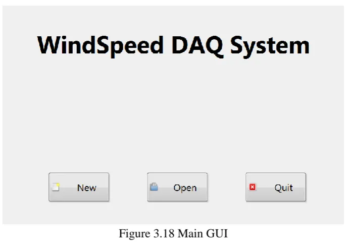
3.3 Software for Instrumentation Operation 43
CHAPTER 4: FLOW QUALITY OF EMPTY WIND TUNNEL 49
4.1 Wind Tunnel Speed Range 49
4.2 Measurement in Empty Wind Tunnel 50
4.2.1 Coordinate system and measurement planes 51
4.2.2 Horizontal profiles of streamwise wind speed 54
4.2.3 Vertical profiles of streamwise wind speed 60
4.2.4 Turbulence intensity 62
4.2.5 Identification of noise sources 64
4.3 Summary for the evaluation of the empty CFI wind tunnel quality 71
CHAPTER 5: FLOW CHARACTERISTICS IN WIND TUNNEL WITH THE
ADDTION OF PASSIVE DEVICES
73
5.1 Design of Passive Devices 73
5.1.1 Design of Spires 74
5.1.3 Testing cases 78
5.2 Effect of spires on the flow characteristics 79
5.3 Effect of roughness elements on flow characteristics 88
5.4 Combined effect of spires and roughness elements on flow characteristics 94
5.4.1 Three spires with 72 pieces of roughness elements (2% frontal area
density)
96 5.4.2 Three spires with 144 pieces of roughness elements (4% frontal area
density)
100 5.4.3 Three spires with 200 pieces of roughness elements (frontal area den
sity of 5.56%)
104
5.5 Summary 109
CHAPTER 6: CONCLUSIONS AND RECOMMENDATIONS 114
6.1 Conclusions 114
6.2 Recommendations 116
REFERENCES 117
APPENDIX A: SUMMARY OF VELOCITY SAMPLE UNCERTAINTY 122
APPENDIX B: LABVIEW® PROGRAMS 123
LIST OF FIGURES
Figure 1.1 CFI wind tunnel at the University of Windsor 1
Figure 1.2 Layout of CFI wind tunnel at the University of Windsor 2
Figure 1.3 Turntable and traverse system 2
Figure 1.4 7-Blade axial flow fan 3
Figure 1.5 Honeycomb screen 3
Figure 2.1 Atmospheric boundary layer 7
Figure 2.2 Logarithmic wind velocity profile (after Garratt, 1992) 9
Figure 2.3 Surface roughness dimensions (after Grimmond and Oke, 1999) 12
Figure 2.4 Mean and fluctuating components of a wind velocity time history 19
Figure 2.5 Vibrating spires (Pang and Lin, 2008) 23
Figure 2.6 Arrangement of the grid and coordinate system (after Owen, 1957) 24
Figure 2.7 Schematic diagram of the array of differentially spaced flat plates in
wind tunnel (after Phillips, 1999)
25
Figure 2.8 Shape of elliptic wedge generator 26
Figure 2.9 Six inch standard half-width spires (Standen, 1972) 27
Figure 2.10 Shapes of spires (Standen, 1972) 27
Figure 3.1 Schematics of instrumentation setup 29
Figure 3.2 Pitot static tube 30
Figure 3.3 Multi-point fitting curve 34
Figure 3.4 CTA measurement chain (1.Hot-wire probe (55P16); 2. 4m cable; 3. Mini
CTA 54T30; 4. Power cable; 5. Data cable)
Figure 3.5 Calibration system of hot-wire probe (1. Pitot static tube; 2. Hot-wire
probe (55P16);3. Jet nozzle; 4. Pressure regulator; 5. Pressure gauge; 6.
Switch; 7. AfterFilter)
35
Figure 3.6 The probe 55P16 fixture (1. Probe 55P16; 2. Clamp; 3. 1. ―Z‖-shaped
rod)
36
Figure 3.7 Clamp 36
Figure 3.8 Close-up of the three clamps 37
Figure 3.9 ―Z‖-shaped rod 37
Figure 3.10 Minimum distance to the floor 38
Figure 3.11 Two-axis BiSlide® traverse system 39
Figure 3.12 ―T‖-shaped plate support 39
Figure 3.13 Cleat and steel plate 40
Figure 3.14 Y-Z mounting 40
Figure 3.15 NI cDAQ-9178 41
Figure 3.16 NI 9222 41
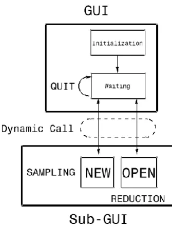
Figure 3.17 State chart 44
Figure 3.18 Main GUI 45
Figure 3.19 Data acquisition GUI 45
Figure 3.20 Use SETTING button to setup the ambient and sampling parameters 46
Figure 3.21 TEST 46
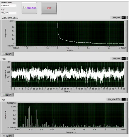
Figure 3.22 Data reduction GUI 47
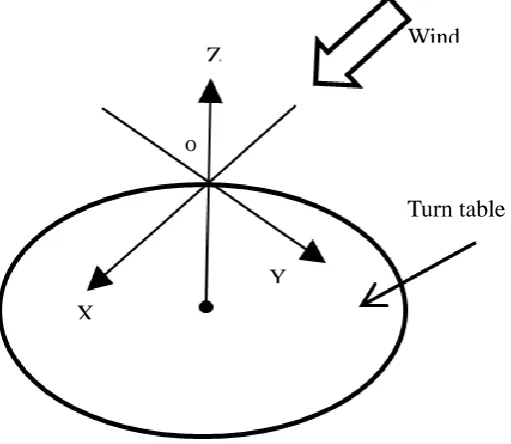
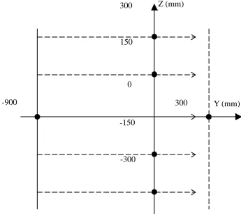
Figure 4.2 Definition of the coordinate system 51
Figure 4.3 Locations of test planes along Z-axis 52
Figure 4.4 Locations of test planes along Y-axis 53
Figure 4.5 Horizontal profile of streamwise wind speed in the empty wind tunnel
(x=0) (Pitot static tube)
55
Figure 4.6 Minimum required sampling number for mean wind speed at sampling
frequency of 32 kHz
56
Figure 4.7 Minimum required sampling number for σ of mean wind speed at sam-pling frequency of 32 kHz
56
Figure 4.8 Horizontal profile of streamwise wind speed (hot-wire anemometer)
(X=0, Z=0)
57
Figure 4.9 Schematics of traverse vertical axis movement and the setup of the
Z-shaped rod
58
Figure 4.10 Schematics of the adjusted installation of Z-shaped rod and HWA 59
Figure 4.11 Horizontal profile of streamwise wind speed after adjustment of Z-rod
orientation (X=0, Z=0)
59
Figure 4.12 Vertical profiles of streamwise wind speed (Pitot static tube) (X=0) 61
Figure 4.13 Vertical profiles of streamwise wind speed (hot-wire anemometer) (X=0) 62
Figure 4.14 Vertical profile of turbulence intensity without noise treatment (X=0,
Y=0)
63
Z=0)
Figure 4.16 A segment of sample wind speed PSD 64
Figure 4.17 Location A 65
Figure 4.18 Location B 65
Figure 4.19 Flexible connector between the fan house and the test section 66
Figure 4.20 Intersection of three data cables 67
Figure 4.21 Mean wind speed oscillates at a low frequency 69
Figure 4.22 Vertical profile of turbulence intensity (X=0) 70
Figure 4.23 Horizontal profile of turbulence intensity (X=0) 71
Figure 5.1 Rectangular working sections as a control volume (Irwin, 1979) 75
Figure 5.2 Wooden triangular spire (mm) 77
Figure 5.3 Bottom surface of a cubic roughness element with two magnet parts
(mm)
79
Figure 5.4 Three spires at the entrance of the wind tunnel test section 80
Figure 5.5 Vertical profiles of streamwise wind speed in the empty wind tunnel and
after installing three spires (X=0, Y=0)
81
Figure 5.6 Vertical profiles of turbulence intensity in the empty wind tunnel and
af-ter installing three spires (X=0,Y=0)
82
Figure 5.7 Vertical profiles of streamwise wind speed after installation of three
spires
83
Figure 5.9 Comparison of dimensionless Vertical profiles of streamwise wind speed
(X=0)
85
Figure 5.10 Dimensionless wind speed fitting curve (X=0, Y=0) 85
Figure 5.11 Horizontal profile of streamwise wind speed (three-spires) (X=0, Z=-700
mm)
86
Figure 5.12 Horizontal profiles of turbulence intensity (three-spire) (X=0, Z=-700
mm)
87
Figure 5.13 Arrangement of roughness element (Case 3) 89
Figure 5.14 Vertical profiles of streamwise wind speed with 200 pieces of roughness
element (frontal area density of 5.5%) (X=0)
89
Figure 5.15 Vertical profiles of turbulence intensitys with 200 pieces of roughness
element (frontal area density of 5.5%) (X=0)
90
Figure 5.16 Vertical profiles of streamwise wind speed with 144 Pieces of roughness
element (frontal area density of 4%) (X=0)
90
Figure 5.17 Vertical profiles of turbulence intensitys with 144 pieces of roughness
element (frontal area density of 4%) (X=0)
91
Figure 5.18 Vertical profiles of streamwise wind speed with 72 Pieces of roughness
element (frontal area density of 2%) (X=0)
91
Figure 5.19 Vertical profiles of turbulence intensitys with 72 Pieces of roughness
element (frontal area density of 2%) (X=0)
92
Figure 5.20 Comparison of vertical profiles of streamwise wind speed (empty tunnel
v.s. three roughness-element-only cases, X=0, Y=0)
Figure 5.21 Comparison of turbulence intensity profiles (empty v.s. three
rough-ness-element-only cases, X=0, Y=0)
93
Figure 5.22 Schematic layout of using spires combined with roughness elements to
simulate atmospheric boundary layer in wind tunnel (mm)
94
Figure 5.23 Actual layout of three spires combined with 200 roughness elements in
the CFI wind tunnel
95
Figure 5.24 Vertical profile of streamwise wind speed (three spires with 72 pieces of
roughness elements, X=0, Y=0)
97
Figure 5.25 Vertical profiles of turbulence intensity (three spires with 72 pieces of
roughness elements, X=0, Y=0)
97
Figure 5.26 Vertical profile of streamwise wind speed fitting curve (three spires with
72 pieces of roughness elements, X=0, Y=0)
98
Figure 5.27 Horizontal profile of streamwise wind speed (three spires with 72 pieces
of roughness elements, X=0, Z=-400 mm)
98
Figure 5.28 Horizontal turbulence intensity (three spires with 72 pieces of roughness
elements, X=0, Z=-400 mm)
99
Figure 5.29 Vertical profile of streamwise wind speed (three spires with 144 pieces
of roughness elements, X=0, Y=0)
101
Figure 5.30 Vertical turbulence intensity (three spires with 144 pieces of roughness
elements, X=0, Y=0)
Figure 5.31 Vertical profile of streamwise wind speed fitting curve (three spires with
144 roughness elements, X=0, Y=0)
102
Figure 5.32 Horizontal profile of streamwise wind speed (three spires with 144
roughness elements, X=0, Z=-400 mm)
102
Figure 5.33 Horizontal turbulence intensity (three spires with 144 roughness
ele-ments, X=0, Z=-400 mm)
103
Figure 5.34 Vertical profile of streamwise wind speed (three spires with 200 pieces
of roughness elements, X=0, Y=0)
105
Figure 5.35 Vertical profiles of turbulence intensity (three spires with 200 pieces of
roughness elements, X=0, Y=0)
106
Figure 5.36 Vertical profile of streamwise wind speed fitting curve (three spires with
200 pieces of roughness elements,X=0, Y=0)
106
Figure 5.37 Horizontal profile of streamwise wind speed (three spires with 200
piec-es of roughnpiec-ess elements, X=0, Z=-400 mm)
107
Figure 5.38 Horizontal profiles of turbulence intensity (three spires with 200 pieces
of roughness elements, X=0, Z=-400 mm)
107
Figure 5.39 Power spectrum at point (0, 0, 0) 108
Figure 5.40 Integral length scale on vertical middle plane (X= 0 mm, Y= 0 mm) 108
sive device arrangement (X=0, Y=0)
Figure 5.42 Vertical profiles of turbulence intensitys under different types of passive
device arrangement (X=0, Y=0)
111
Figure 5.43 Comparison between power law wind speed profile with exponent 0.33
and the dimensionless vertical profiles of streamwise wind speed under
different frontal area density of the roughness elements
112
Figure 5.44 Relation between frontal area density of roughness element and exponent
α of power law wind speed profile
113
Figure 5.45 Hypothetic curve between α-value and frontal area density 113
LIST OF TABLES
Table 2.1 Terrain Classification 10
Table 2.2 Aerodynamic properties of surfaces (Monteith and Unsworth, 1990) 14
Table 2.3 Terrain roughness category and exposure type (ASCE 7-95) 18
Table 2.4 Constants c and d for different terrain types 20
Table 3.1 Multi-point Calibration 34
Table 4.1 Accelerations at different locations and motor frequencies 66
NOMENCLATURE
A,B, n constants in the King’s law
constants in the unicurve transfer function
𝑃
̅̅̅̅ block top surface area
total frontal area of all spires
𝑇
̅̅̅̅ block floor area
b base of the triangle
calibration coefficients for hot-wire probe
drag coefficient of each spire
effective surface friction coefficient
d zero-plane displacement, or the width of a wind tunnel
DAQ Data Acquisition
𝐷𝑥 length of the influence area of a block
𝐷𝑦 width of the influence area of a block
𝑑𝑢̅
𝑑𝑧 shear of the mean wind speed
E anemometer voltage
E(f) energy of an eddy
cut-off frequency of a low-pass filter
height of a wind tunnel
h height of spires
𝐼, 𝐼𝑢 turbulence intensity
𝑘 Von Kármán constant
𝑙𝑚 mixing length
𝐿 Obukhov length
𝐿𝑥 length of the block
𝐿𝑦 width of the block
N sampling number
Ns number of spires
𝑦 𝑚 velocity pressure
( ) auto-correlation function
𝑢(𝑘) power spectrum density
SR sampling rate
T sampling time
T1 integral time scale
t0 sampling starting time
𝑣̅ lateral wind speed
𝑢𝑟 known wind speed at a reference height
𝑢(𝑧) wind speed at height z
𝑢̅ longitudinal mean wind speed
𝑢′ longitudinal fluctuating component
𝑢∗ friction (or shear) velocity
𝑢𝑟𝑚 , 𝜎 longitudinal turbulence strength
𝑈̅ mean wind speed
𝑈 value of U above the boundary layer
𝑢′𝑤′
̅̅̅̅̅̅ constant momentum flux
distance from station 2 to station 3
𝑤̅ vertical fluctuating component
𝑤′ vertical fluctuating component
( ) time series sampled according to the Nyquist criteria
z height above tunnel floor
𝑧 surface roughness length
𝑧𝐻
̅̅̅ height of the block
Greek Symbols
ʌ𝑥 longitudinal length scale
height of boundary layer
ρ air density
( ) auto-correlation coefficient of the samples
𝜓 stability term
energy cascade rate
𝜆̅ roughness frontal area density
λp
̅̅̅ roughness plan area density
CHAPTER 1 INTRODUCTION
1.1 Background
Wind tunnel is an important research tool in the field of wind engineering. It has an
extensive application, which includes studying wind-induced load on and response of
structures, investigating wind-related environmental issues, evaluating pedestrian level
wind comfort and assessing aerodynamics feature of vehicles. Compared to full-scale
measurement, the cost of wind tunnel test is much lower. In addition, under controllable lab
conditions, test is repeatable which ensures the accuracy of the results. Thus, wind tunnel
tests remain as the most popular measure to obtain wind-related information.
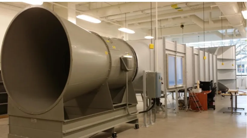
A new wind tunnel granted by Canada Foundation for Innovation (CFI) was
con-structed at the University of Windsor in December, 2012 (Figure1.1). It will be referred as
the CFI wind tunnel in the rest of the document. This is an open-loop low-speed
atmos-pheric boundary layer wind tunnel, designed to perform aerodynamic studies of various
civil structures and wind-related environmental issues.
Figure 1.2 illustrates the overall layout of the CFI wind tunnel. As can be seen from
the figure, this wind tunnel has a total length of 17.6m. It consists of the inlet bell, the
con-traction part, the flow development region, the test section, the transition part, the fan house
and the diffuser. The size of the test section is 1.8 m wide by 1.8 m high.
Figure 1.2 Layout of CFI wind tunnel at the University of Windsor
On the floor of the test section, there is a turn table with a diameter of 1.5m, as
giv-en in Figure 1.3. It can be rotated by 360. By mounting models on the turn table and
rotat-ing it, it allows to simulate the scenario of wind blowrotat-ing from different directions on the
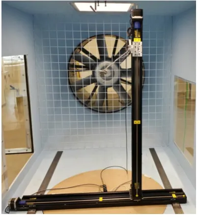
testing model. The airflow is generated by a 7-blade axial-flow fan which has a diameter of
1.7m.
The electric motor of the fan, shown in Figure 1.4, has a power of 110 kw.
Honey-comb screen is mounted at the end of the inlet contraction part. It is used to reduce large
turbulent eddies. As can be seen from Figure 1.5, the honeycomb has hexagonal shape and
the thickness of the screen is 12 mm. The designed maximum wind velocity at the test
sec-tion is 15m/s.
Figure 1.4 7-Blade axial flow fan
Figure 1.5 Honeycomb screen
1.2 Motivation
The CFI wind tunnel is a new facility. It is necessary to set up all required
instru-mentations and evaluate the flow quality in the empty tunnel prior to any other tests. In
envi-ronmental issues. These all occur within the atmospheric boundary layer close to the
ground surface, where various man-made structures and other obstacles are present.
De-pending on the terrain condition, the characteristics of the approaching wind could be
con-siderably affected. When studying wind-induced effects on structures in the wind tunnel, it
is of utmost importance to faithfully reproduce the terrain condition at the site. It is usually
achieved by setting up passive devices in the upstream of the test section. The effect of
dif-ferent types of passive device and their various combinations on the flow characteristics at
the test section needs to be studied and properly understood in order to successfully
simu-late atmospheric boundary layer flow associated with different terrain conditions.
1.3 Objectives
The objectives of the current project are as follows:
1. Set up instrumentations in the CFI wind tunnel. Design and manufacture fixtures and
clamps used to support Pitot static tube and hot-wire anemometer. Develop a new
data acquisition system for these sensors and software for data sampling and
treat-ment.
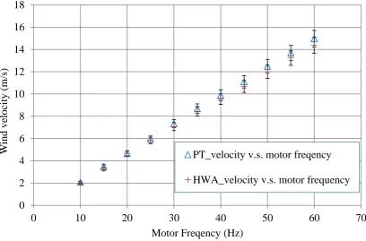
2. Evaluate the flow quality in the empty wind tunnel. Determine the relation between
the fan motor frequency and the generated wind speed, as well as the maximum
achievable wind speed of the CFI wind tunnel. Examine the uniformity and
sym-metry of the flow field at the testing section and the free stream turbulence intensity
level.
to be used in the simulation of atmospheric boundary layer in the CFI wind tunnel.
4. Study the impact of different passive device arrangements on the flow characteristics
in the wind tunnel. The testing cases will include: spires-only,
rough-ness-elements-only, and the combination of spires and roughness elements.
5. Verify Irwin’s approach for spire design in terms of spire height and the generated
boundary layer thickness.
6. Explore the relation between the exponent in the power law mean wind speed profile
CHAPTER 2 LITERATURE REVIEW
Wind tunnel is an important tool used in aerodynamic research to study the effects
of air past solid objects. The earliest wind tunnels were built in the late 19th century when
many attempted to invent successful heavier-than-air flying machines. Later, the scope of
wind tunnel study was much expanded to other areas. For example, to study the effects of
wind on man-made structures or objects, to investigate wind-related environmental issues
such as air pollution, soil erosion and snow drifting. In these kinds of studies, it is required
to simulate the interaction between the wind and the objects submerged in the lowest few
hundred meters of the atmosphere. This layer is known as the surface layer, which is the
bottom layer of the atmospheric boundary layer (ABL). The wind tunnel designed for this
purpose is called atmospheric boundary layer wind tunnel (ABLWT). In this chapter, the
fundamentals and theories of ABL will be reviewed, followed by the various approaches of
designing an ABLWT.
2.1 Atmospheric Boundary Layer
The characteristics of ABL are directly influenced by its contact with the ground
surface, the temperature, and the humidity of air. In a clear day, the ABL can be typically
divided into several sub-layers. The bottom sub-layer is called the surface layer. Due to
presence of various obstacles on the ground surface, wind flow close to the ground would
be retarded. Thus, there is a vertical gradient in the wind speed distribution. Commonly, it
Figure 2.1 Atmospheric boundary layer
Logarithmic wind velocity profile
Majority of the human activities occur in the surface layer. Despite the effect of a
complex ground surface on turbulent flow, the theory of the surface layer is more
devel-oped than that for the boundary layer as a whole because the presence of ground surface
limits the size of the eddies. Further, a large number of ground-based measurement
cam-paigns have been carried out using instrumented masts. Within the surface layer, turbulent
fluxes of heat and momentum are usually assumed as constants. For example, in the case of
a convective boundary layer, the sensible heat flux at the top is typically 90% of the ground
value. Thus, it is reasonable to assume it to be constant through the surface layer. Similar
reasoning applies to momentum, and the constant momentum flux 𝑢̅̅̅̅̅̅′𝑤′ is defined as
𝑢∗ = √−𝑢̅̅̅̅̅̅ (2.1)′𝑤′
where 𝑢∗ is the friction (or shear) velocity, typically around 0.2𝑚/𝑠 in the day and 𝑢̅̅̅̅̅̅′𝑤′
is always negative in the surface layer, 𝑢′ and 𝑤′are respectively fluctuating components
of the horizontal and vertical velocity.
Prandtl (1904) developed a model, in terms of mixing length, to describe
by means of an eddy viscosity. The mixing length 𝑙𝑚 is the typical depth of a surface layer
in the vertical direction. Actually, a surface layer is much shallower than its width, thus the
mixing length can be considered as the radius of a typical eddy. This leads to the following
relationship between the friction velocity, the mixing length and the shear of the mean wind
in the surface layer:
𝑢∗ = 𝑙𝑚
𝑑𝑢̅
𝑑𝑧 (2.2)
Since 𝑢∗is a constant along height, if 𝑙𝑚is known, then the wind shear and hence the
ver-tical wind speed variation can be determined. As discussed earlier, when the flus
Richard-son number equals to zero, the surface layer becomes neutral and stable. The variation in
the potential temperature, which is the temperature that a parcel of air would have if it
brought adiabatically to some reference pressure, would not play an active role. It turns out
that the mixing length would only dependent on the reference height 𝑧, and the eddy size
would increase linearly with respect to height, i.e.
𝑙𝑚 = 𝑘𝑧 (2.3)
where 𝑘 is the Von Kármán constant.
Substitute Eq. (2.3) into Eq. (2.2) yields
𝑑𝑢̅ 𝑑𝑧 =
𝑢∗
𝑘𝑧 (2.4)
If assume that the wind speed is zero at height 𝑧 , and integrate Eq. (2.4), it gives
∫ 𝑑𝑢̅ 𝑢(𝑧) =𝑢∗ 𝑘 ∫ 𝑑𝑧 𝑧 𝑧 𝑧 𝑢(𝑧) =𝑢∗ 𝑘 ln (
𝑧
𝑧 ) (2.5)
where 𝑘 is the Von Kármán constant, which is roughly 0.4 for all turbulent fluids, 𝑧 is
logarithmic profile falls to zero. Eq. (2.5) describes the logarithmic wind velocity profile, as
shown in Figure 2.2
Figure 2.2 Logarithmic wind velocity profile (after Garratt,1992)
When wind blows over an array of densely packed objects, such as a forest, a city,
and so on, an offset in height should be introduced so that the wind velocity profile moves
upward by a displacement d. Thus Eq. (2.5) becomes:
𝑢(𝑧) = 𝑢∗ 𝑘 ln (
𝑧 − 𝑑
𝑧 ) (2.6)
where d is the zero-plane displacement.
Under non-neutral conditions, a stability term,𝜓, is introduced to Eq.(2.6), i.e.
𝑢(𝑧) =𝑢∗ 𝑘 ln (
𝑧 − 𝑑
𝑧 ) + 𝜓(𝑧 𝑧 𝐿) (2.7)
where 𝐿 is the Obukhov length and 𝜓 is a stability term.
Although the mixing length model is only a rough approximation, the logarithmic
wind velocity profile has been verified by many field data measured by different
research-ers. In the lowest 10 to 20 m of the surface boundary layer, the logarithmic wind velocity
varia-tion. To gain more insights into the characteristics within the surface layer, the key
parame-ters governing the logarithmic wind velocity profile will be reviewed respectively.
Surface Roughness Length z
Surface roughness length z is equivalent to the height at which the wind speed
theoretically becomes zero in a logarithmic profile. In reality, wind speed at this height no
longer follows the mathematical description of the profile. It is named such that it is
typi-cally related to the height of terrain roughness elements. Although this is not a physical
length, it can be considered as a length scale representing the roughness of the surface. As
an approximation, it is roughly one-tenth of the height of the surface roughness elements.
Table 2.1 lists the relation between some typical terrain conditions and the corresponding
roughness length.
Table 2.1 Terrain Classification
Terrain Description
Roughness Length
z (m)
Literature
Open sea, fetch at least 5 km 0.0002 Lewis,1976
Mud flats, snow; no vegetation, no obstacles 0.005 Callaghan,1976
Open flat terrain; grass, few isolated obstacles 0.03 ESDU, 1972
Low crops; occasional large obstacles 0.1 Deacon, 1953
High crops; scattered obstacle 0.25 Leurs, 1981
parkland, bushes; numerous obstacles 0.5 Garratt, 1978
Regular large obstacle coverage 1.0 Allen, 1976
Despite the progress in the past few decades to use surface roughness length to
ac-count for the effects of ground surface covered with small roughness elements on the wind
velocity profile, due to high cost of field measurements, much effort has been made to find
a better model to reproduce the wind velocity profile in ABLWT. This is typically achieved
by the combined use of turbulence generation devices, such as spires, and roughness
ele-ments.
Refer to Figure 2.3, the roughness plan area density λ̅̅̅p is defined as the ratio
be-tween the block top surface area ̅̅̅̅𝑃 and the block floor area ̅̅̅̅𝑇, i.e.
𝜆𝑃 ̅̅̅ =̅̅̅̅𝑃 𝑇 ̅̅̅̅= 𝐿𝑥 ̅̅̅ 𝐿̅̅̅𝑦 𝐷𝑥
̅̅̅̅ 𝐷̅̅̅̅𝑦 (2.8)
where 𝐿𝑥is the length of the block (along the wind direction);
𝐿𝑦 is the width of the block (transverse to the wind direction);
𝐷𝑥is the length of the influence area of a block (along the wind direction);
𝐷𝑦 is the width of the influence area of a block (transverse to the wind direction);
and the roughness element frontal area density 𝜆̅ is defined as:
𝜆̅ =̅̅̅̅𝐹
𝑇
̅̅̅̅= 𝑧𝐻 ̅̅̅ 𝐿̅̅̅𝑦
𝐷̅̅̅̅ 𝐷𝑥̅̅̅̅𝑦 (2.9)
where 𝑧̅̅̅ 𝐻is the height of the block;
Lettau (1969) depicted the relation between the surface roughness length and the
alignment of roughness elements along the wind tunnel floor based on wind tunnel testing
results, which was
𝑧 =1
Figure 2.3 Surface roughness dimensions (after Grimmond and Oke, 1999)
In the experimental study by Counihan (1971), roughness cubes were placed in
dif-ferent alignments downwind of elliptic wedge eddy generators. By analyzing the velocity
profiles, an empirical formula different from Lettau's was proposed:
𝑧 = 𝑧̅̅̅[1.08𝜆𝐻 ̅̅̅ − 0.08] (2.11)𝑃
The empirical formula proposed by Lettau (1969) is applicable to λ̅̅̅ < 0.06p , whereas that
by Counihan (1971) is valid for 0.1 <λ̅̅̅ < 0.25p .
In the empirical formula proposed by Jackson (1981), the surface roughness length
is determined by the roughness frontal area density 𝜆̅, the drag coefficient , the
rough-ness element height 𝑑, and the mixing length 𝑙 𝑜𝑟 𝑙ℎ:
𝑧̅𝐻− 𝑑
𝑧 = 𝑒𝑥𝑝 | 𝜅ℎ 𝛼𝑙ℎ
| (2.12)
where 𝛼 = 𝜆̅ 𝑧̅𝐻 /4𝑙
Theurer (1993) introduced the roughness plan area density λ̅P in his roughness
length prediction model and found that Lettau’s formulation of z would fail for plan area
density higher than 0.25. Wieringa (1993) pointed out the deficiencies in these empirical
wind tunnel testing data, Peterson (1997) noticed that uncertainty in the prediction of wind
velocity profile could occur due to selection of different fitting range of data along height.
This implies that the effect of zero-plane displacement on the surface roughness length
cannot be neglected. A comparison between these empirical models showed that all of them
are valid under the conditions of high roughness frontal or plane area density (Duijim,
1999). Bottema (1997) developed a new model to deal with cases of low roughness frontal
or plane area density, or non-uniform dimensions of roughness elements. Results showed
that the consistency between Bottema's and Lettau's model was up to 95%.
The empirical formulae reviewed above are all developed based on wind tunnel
testing results. Before 1998, it was believed that the velocity profile was strongly dependent
on properties of roughness elements, such as dimension, shape, and alignment on a wind
tunnel floor. Since these formulae still cannot satisfactorily predict the velocity profile,
fur-ther improvements were proposed by different researchers by introducing anofur-ther
parame-ter, which is the zero-plane displacement d. In the refined formulae proposed by Macdonald
et al (1998), besides dimension and alignment of roughness elements as well as the
ze-ro-plane displacement, two new parameters, i.e. the drag coefficient and the von Kármán
constant were included based on the principle of conservation of momentum. Jia et al (1998)
found that when the roughness frontal area density was reduced by over 20%, the surface
roughness length would decrease. This agrees with the finding by Rapauch and Thom
(1980).
It can be seen from the above literature that surface roughness length, which
velocity profile. When simulating such an effect in the wind tunnel using cubic roughness
elements, the dimension, shape and alignment of roughness elements would strongly affect
the generated wind velocity profile. In the current study, cubic roughness elements will be
used as part of the passive device to produce natural atmospheric boundary layer above
certain type of terrain condition in the CFI wind tunnel.
Zero-plane displacement d
Thom and Raupach (1981) defined the zero-plane displacement, d, as the height in
meters above ground where wind speed becomes zero as a result of the presence of
obsta-cles such as trees and buildings. In practice, it is evaluated from the logarithmic wind
pro-file by plotting the logarithm of height versus wind speed under near neutral conditions.
Table 2 gives the zero-plane displacement associated with a number of typical ground
sur-face types.
Table 2.2 Aerodynamic properties of surfaces (Monteith and Unsworth, 1990)
Surface Roughness Length(m) Zero Plane Displacement (m)
water 0.1-10-4 N/A
ice N/A
snow N/A
sand 0.0003 N/A
soil 0.001-0.01 N/A
grass, short 0.001-0.003 < 0.07
grass, tall 0.04-0.1 < 0.06
crops 0.04-0.2 < 3
orchards 0.5-1 < 4
deciduous forest 1-6 < 20
On the other hand, the zero-plane displacement can be considered as the height at
which the mean drag appears to act (Jackson, 1981). Stull (1988) estimated that the
ze-ro-plane displacement should vary between 0.6 to 0.8 times the height of the forest
cano-pies. The results by Arya (1998) verified Stull's prediction. However, the roughness length
and zero-plane displacement yielded from measurement results over agricultural crops and
forests are not consistent, since the latter has distinct and different leaf area profiles. From a
theoretical perspective, Shaw and Pereira (1982) used a higher order turbulence closure
model to examine the inter-relation between the zero-plane displacement, the surface
roughness length, the leaf area index, the canopy drag and the distribution of leaf area.
Theurer (1993) normalized the zero-plane displacement by the roughness element
height. It was found that the dimensionless zero-plane displacement was 1.67 times of the
roughness frontal area density 𝜆 . This convinced many researchers that the conventional
empirical models of surface roughness length should be corrected by the zero-plane
dis-placement. To further confirm this, Spanton et al (1996) conducted a series of field
meas-urements to obtain roughness frontal area density at different districts in some cities in UK.
Results showed that 𝜆 is 50-60% in business zones and 20-40% in industrial zones. This
suggests that the Lettau's model, of which the effect of zero-surface displacement is
ne-glected, would overestimate the surface roughness length. After comparing data yielded
from seven different calculation methods, Peterson (1997) indicated that the zero-plane
displacement should be included in the surface roughness length calculation model.
Shear velocity μ∗ is a scaling velocity that is related to momentum transfer. It is an
important parameter in geophysical flows. It is typically derived from logarithmic flow
ve-locity profile by applying ordinary least square regression. This parameter would also
strongly affect the calculation results of surface roughness length (Bottema et al, 1998).
Raupach and Thom (1980) indicated that due to the uncertainty of turbulent kinetic energy,
the calculated μ∗ is different from the measurement. Thus, the approach of using turbulent
kinetic energy to determine μ∗is hardly used now. Cook (2003) noticed a 15% discrepancy
in the shear velocities measured by Iyengar and Farell (2001). According to his speculation,
this could be caused by the drag acting on a block could not be totally converted into inner
Reynolds stress. The correct approach is to measure Reynolds stress directly. A number of
new methods for calculating shear velocity have been proposed recently. Liu et al (2003)
measured the turbulence intensity close to a wind tunnel wall and then substituted the
sur-face roughness length into the velocity profile formula to obtain shear velocity. In the
mod-el proposed by Hollingsworth (2003), various free stream parameters, such as the mean
flow velocity, the integral length scale and the turbulence intensity were all considered in
the formulation.
Power-law wind velocity profile
The power-law wind velocity profile is often used as a substitute for the logarithmic
wind velocity profile in non-complex terrain up to a height of about 200 m above ground
level. It can be expressed as:
𝑢(𝑧) 𝑢𝑟 = (
𝑧 𝑧𝑟)
where 𝑢(𝑧) is the wind speed (in 𝑚/𝑠) at height z (in meter);
𝑢𝑟is the known wind speed at a reference height 𝑧𝑟;
𝛼 is an exponent, which typically varies from about 0.1 on a sunny afternoon to
about 0.6 during a cloudless night. Under neutral stability conditions, it is approximately
1/7, or 0.143.
In wind resource assessments, a constant α value of 1/7 is commonly assumed.
However, when a constant power law exponent is used, the surface roughness length, the
zero-plane displacement (Touma, 1977), or the stability of the atmosphere (Counihan, 1979)
are excluded in the prediction of velocity profile. In places where trees or structures impede
the near-surface wind, this may yield quite erroneous estimates. Even under neutral
stabil-ity conditions, an exponent of 0.11 is more appropriate to be used for the over open water
(e.g. for offshore wind farms) than 0.143, which is more suitable for terrain over open land
surfaces (Meindl and Gilhousen, 1994). The larger the power-law exponent is, the more
considerable the gradient in the vertical profile of streamwise wind speed will be. The four
types of terrain roughness categories implied by Exposures A, B, C and D in ASCE 7-95
are given in Table 2.3.
Although power-law is a useful engineering approximation to estimate the average
wind speed profile, the actual profile deviates from this idealized relationship. As discussed
by Irwin (1979), the exponent in the power-law wind velocity profile is a function of
stabil-ity, surface roughness length and the height range within which it is determined. In the
lowest 10–20 m of the planetary boundary layer, the logarithmic profile can generally offer
power-law profile has a wider applicable range. Bergstom (2001) conducted open duct
tur-bulent experiments on smooth and coarse walls. The friction velocity was determined by
the power-law profile since it was noticed that the logarithmic profile layer was very thin
and could be neglected. Afzal (2001) studied a turbulent boundary layer without neglecting
pressure gradient. It was found that the transient layer could be described by either the
power-law or the log-law. In particular, as Reynolds number increases, the power-law
pro-file and logarithmic propro-file coincides with each other.
Turbulence Intensity
Turbulence in natural wind causes fluctuation of wind velocity in time and space.
Figure 2.4 shows a segment of typical wind velocity time history.
The movement of wind is comprised of three velocity components, which are along
respectively the three Cartesian coordinate axis directions x, y and z. 𝑢 is the horizontal
stream wise velocity, 𝜈 is the horizontal lateral velocity and 𝑤 is the vertical velocity.
These three velocity components can be further expressed as the superposition of a mean
component and a zero-mean fluctuation component (Reynolds’ averaging), i.e. Table 2.3 Terrain roughness category and exposure type (ASCE 7-95)
Exposure type Terrain Description α z (m)
D Open sea, Fetch at least 5 km 0.12 0.002
C Mud flats, snow; no vegetation, no obstacles 0.16 0.02
B parkland, bushes; numerous obstacles 0.22 0.5
𝑢 = 𝑢̅ + 𝑢′ 𝜈 = 𝜈̅ + 𝜈′ 𝑤 = 𝑤̅ + 𝑤′
} (2.14)
where, 𝑢̅ 𝑣̅ 𝑤̅ are mean components of velocity, and 𝑢′ 𝑣′ 𝑤′ are the fluctuating
components of velocity. In the case of vertical velocity, its mean component is typically
zero over flat terrain.
Figure 2.4 Mean and fluctuating components of a wind velocity time history
The mean wind speed is defined as:
𝑈̅ =1
𝑇∫ 𝑈𝑑𝑡
𝑡 +𝑇
𝑡 𝑇
= 1
𝑁∑ 𝑈(𝑑𝑖𝑠𝑐𝑟𝑒𝑡𝑒)
𝑁
=
= (𝑢̅̅̅̅̅̅̅̅̅̅̅̅̅̅̅̅̅̅̅̅+ 𝜈 + 𝑤 ) ⁄
= (𝑢̅ + 𝜈̅ + 𝑤̅ + 𝑢̅̅̅̅̅̅ + 𝜈′𝑢′ ̅̅̅̅̅ + 𝑤′𝜈′ ̅̅̅̅̅̅̅)′𝑤′ ⁄
(2.15)
where T is sampling time, t0 is sampling starting time, N is sampling number, and the
lon-gitudinal turbulence strength is
𝑢𝑟𝑚 = 𝜎 = √𝑢̅′ = √1
𝑁∑(𝑢′)
𝑁
=
(2.16)
Turbulence is often considered as the superposition of eddies with different sizes
transported by the mean flow. One of the main characteristics of turbulence is the
the root-mean-square of the fluctuating component of the longitudinal wind velocity and its
time-averaged mean value, i.e.
𝐼 = 𝜎 𝑈⁄ (2.17)̅
Similar definitions can be applied to the lateral and vertical velocities.
An empirical formula for estimating turbulence intensity of ABL flow is provided
by ESDU 75001 (1975), i.e.
𝐼𝑢 = 1
ln (𝑧 𝑧⁄ )*0.867 + 0.566log𝑧 − 0.246(log𝑧) + 𝜆 (2.18)
𝜆 = { 0.76
𝑧 . 7 𝑧 > 0.02𝑚 1.0 𝑧 ≤ 0.02𝑚
(2.19)
where 𝑧 is the surface roughness length, and z is the height.
Zhou et al (2002) proposed a general formula for estimating the turbulence intensity
of ABL flow, which is
𝐼(𝑧) = 𝑐(𝑧 10⁄ ) (2.20)
where c and d are constants related to the terrain type and are listed in Table 2.4.
Table 2.4 Constants c and d for different terrain types
CODE ASCE 7-95 AS1170.2 NBC RLB-AIJ EUROCODE
Terrain
Class c d c d c d c d c d
A 0.450 0.167 0.453 0.300 0.621 0.360 0.402 0.400 0.434 0.290
B 0.300 0.167 0.323 0.300 0.355 0.250 0.361 0.320 0.285 0.210
C 0.200 0.167 0.259 0.300 0.200 0.140 0.259 0.250 0.189 0.160
D 0.150 0.167 0.194 0.300 0.204 0.200 0.145 0.120
Power Spectrum of Longitudinal Fluctuating Velocity
In the view of Kolmogorov (1941), turbulent motion of flow spans a wide range of
scales from a macro scale at which the energy is supplied, to a micro scale at which energy
is dissipated by viscosity. The interaction between eddies of different scales passes energy
from the larger ones gradually to the smaller ones. This process is known as the turbulent
energy cascade. The atmospheric power spectrum typically consists of three sub-ranges: the
energy containing range, the inertial sub-range, and the dissipation range. Turbulence in the
energy containing range is produced by shear and buoyancy. In the inertial sub-range,
en-ergy is neither produced nor destroyed, but cascades from larger to smaller eddies. Let us
denote as the energy cascade rate. By dimensional analysis, the spectrum in the inertial
sub-range can be obtained as
𝑢(𝑘) = 𝛼 𝑘 (2.21)
where 𝛼 is the Kolmogorov constant, 𝑘 is a wavenumber, defined by 2 / l n .
The value of 𝛼 has been determined experimentally to be about 1.5 (Pope, 2000).
The − 5 3 ⁄ power law of the energy spectrum has been observed to hold well in the inertial
range, that is, for those intermediate size eddies. However, an alternative theory that
pre-dicts a −2 power law has also been proposed (Saffman, 1968; Long, 1997; 2003).
2.2 Simulation of atmospheric boundary layer in wind tunnel
Simulation of atmospheric boundary layer in wind tunnel can be achieved by
natu-ral formation or introducing man-made devices. The former approach requires very long
formed when flow passes a 20-30m long rough floor development section. The boundary
layer wind tunnel at Western university uses this method to simulate ABL. However, this
approach is rarely utilized now due to the requirement of long test section. But rather, the
latter approach, i.e. to form ABL in the wind tunnel using different types of man-made
de-vices, is the primary technique adopted by many researchers in different wind tunnel labs.
Depending on whether or not controllable devices are part of the simulation tool, the latter
approach can be further classified as passive simulation method and active simulation
method. The essential difference between these two is whether or not the device is capable
of supplying energy into the flow field in the wind tunnel. Various man-made devices used
in the passive and active simulation methods to generate ABL in wind tunnel will be
re-viewed in the next two subsections.
2.2.1 Active simulation approaches
Due to limitation of wind tunnel size, it is difficult to generate large scale turbulence
using passive simulation methods. By supplying additional energy with appropriate
fre-quency components to the wind tunnel flow field, the active simulation approaches can
help to increase the low frequency components in turbulent flow, and thus improve the
simulation results on integral length scale and power spectra of longitudinal fluctuating
ve-locity. However, the high cost of active simulation devices limited its utilization in practice.
Nishi et al (1999) reproduced the vertical Reynolds stress coefficient in a two
di-mensional wind tunnel, which had eleven fans arranged vertically. Each fan was connected
length×width×height were respectively 3.8m×0.18m×1.0m and 5.0m×1.0m×1.0 m. The
maximum wind velocity of the tunnel was 11 m/s. Oscillating airfoils were installed at the
mid-section of the tunnel to add vertical turbulence to the main flow. All fans and
oscillat-ing airfoils were controlled independently by computers.
Various types of turbulent flow characteristics could be simulated by modifying the
computer program. Using this kind of active simulation devices, Nishi and his colleagues
also reproduced coherent motions similar to the natural turbulent flow.
The 1MW boundary layer wind tunnel at the Monash University used active
simu-lation techniques to reproduce ABL over suburban terrain in the wind tunnel. A large trip
board with adjustable oscillation stroke and frequency was hinged on the tunnel floor and
activated by a pneumatic cylinder to flap in the wind. Cheung et al (2001) used this active
device to simulate more real atmospheric turbulence effects on large structures and
pollu-tant dispersion studies.
Pang and Lin (2008) developed a technique of using oscillating spires to actively
simulate the turbulent boundary layer (Figure 2.5). A conventional spire is symmetrically
split into two parts, which can flap with a certain frequency. This device was proven to
in-creases the turbulence energy and the integral scale.
2.2.2 Passive simulation approaches
In the passive simulation approach, man-made devices, such as fences, uniform
grids, spires and roughness elements, or combination of some of them, are typically used to
artificially thicken the boundary layer. To reproduce flow characteristics over certain type
of terrain condition at the test section, it is required not only to reproduce the corresponding
wind velocity profile, but the associated turbulence intensity, integral length scale and
power spectra of the longitudinal fluctuating velocity.
Owen (1957) obtained a nearly uniform shear flow in the working section of a wind
tunnel by inserting a grid of parallel rods with varying spacing, as shown in Figure 2.6. By
adjusting arrangements of the rods along the vertical direction, a linear or logarithmic
vari-ation of velocity profile was produced at large distance downstream. However, the
experi-mental results of turbulence intensity disagreed with the theoretical prediction because
dis-sipation of turbulence energy was high.
Figure 2.6 Arrangement of the grid and coordinate system (after Owen, 1957)
Philips et al (1999) used an array of non-uniformly spaced flat plates to produce a
specified velocity profile, which is shown in Figure 2.7. The fully developed duct flow
This method was developed to simulate weak shear flow with zero vertical pressure
gradi-ents.
Figure 2.7 Schematic diagram of the array of differentially spaced flat plates in wind tunnel (after Phillips, 1999)
Ham et al (1998) modified the shape of conventional spires so as to generate a
low-turbulence nominal flow. The geometric shape of spire was discontinuous. Several
rows of chain were used as roughness elements and placed behind an upstream barrier. A
very good agreement between the laboratory and field wind velocity characteristics was
observed.
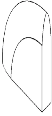
Counihan (1969) developed a method to simulate an ABL in a wind tunnel. The
eddy generators consisted of triangular, cranked triangular, plane elliptic and elliptic wedge
shapes. The shape of the elliptic wedge generator is shown in Figure 2.8. Counihan carried
out an experiment in the CERL boundary layer wind tunnel which has a working section
24" wide, 7-30" high and 5′ long.
The tests were conducted at a free stream velocity of 9m/s and without the presence
of a barrier or surface roughness. Counihan found that a working section length between
general characteristics of boundary layer flow were formed at a distance of three boundary
layer thicknesses from the generator trailing edges. To simulate flow condition over rural
terrain, Counihan's method can produce satisfactory simulation results in wind tunnel.
Figure 2.8 Shape of elliptic wedge generator
Standen (1972) proposed a method to generate thick shear layer using an array of
standard half-width spires. These spires, with spacing of half spire height, were placed at
the entrance to the tunnel working section, as shown in Figure 2.9. Standen made various
investigations by changing the height of spires from 6" to a maximum of 7", and increasing
wind speed from 15m/s to 30m/s. He also developed several other types of spires, as shown
Figure 2.9 Six inch standard half-width spires (Standen, 1972)
Spires shown in Figure 2.10(a) and Figure 2.10(b) are triangular plates without central
sec-tion and Figure 2.10(c) with a rear splitter.
Figure 2.10(a) Figure 2.10(b) Figure 2.10(c)
Figure 2.10 Shapes of spires (Standen, 1972)
Standen's method can provide a good approximation to the ABL up to 450 m above
the ground surface. However, he thought the method need to be refined. Especially, the
ra-tio of boundary layer thickness to spire height is not a constant for all spire sizes.
Irwin (1979) found that Standen's method might produce very high spire drag and a
boundary layer with too high αvalue. At the same time, he thought any roughly triangular
shaped spires would give an acceptable boundary layer simulation at six spire heights
details of the spire shape are not that important. Based on the overall momentum balance at
different stations in the wind tunnel, he introduced a new method to design spires. The
shape of the spire was triangular. A set of spires were placed at the entrance to the test
sec-tion and followed by an array of cubes. The mean velocity profile, longitudinal turbulence
intensity and integral length scale compare well with neutral planetary boundary layer data,
and other turbulence properties, such as turbulence spectrum, are similar to those at full
scale measurements.
Since the spire-roughness element technique was proposed, it was widely used by
many wind tunnel labs to simulate a wide range of surface layer. Although the simulation
data reported by individual projects tend to be scattered and there is no overall assessment
available, they lied almost entirely within the range of the full scale data. So, the eddy
CHAPTER 3 CFI WIND TUNNEL SETUP
3.1 Instrumentations
The wind speed measurement system in the CFI wind tunnel is shown in Figure 3.1.
It includes a Pitot static tube, a Miniature CTA 54T30 Hot-wire anemometer, an NI9222
data acquisition card and a computer. Analogue signals from the Pitot tube and the hot-wire
anemometer are collected firstly into NI9222 and then transferred into the computer. These
signals will be analyzed and treated by software developed in the Labview® environment.
The instrumentations used in the current study are described as follows:
Figure 3.1 Schematics of instrumentation setup
3.1.1 Pitot Static Tube
A Pitot static tube is used to monitor the free stream mean wind speed in the wind
tunnel during tests, which is used as the reference wind speed for analyzing experimental
data. It measures the dynamic pressure of the air by differencing the total pressure and the
static pressure. The static pressure is exerted on the sidewall of the tube whereas the total
pressure (also known as the stagnation pressure) is taken at the point tip of the tube. The
Usually, a Pitot static tube has two tubes, one inside the other, to sense both pressures
sim-ultaneously. By connecting these two tubes differentially to a manometer, the velocity
pressure can be directly obtained and the corresponding air velocity can be determined by
applying the formula
𝑦 𝑚 = 𝑈 (3.1)
where ρ is the air density and U is the air velocity. The maximum accuracy of a Pitot static
tube is ±2% in the laboratory application.
The Pitot static tube used in the CFI wind tunnel is Dwyer® 160E-01. It is made
of304 stainless steel. The outside diameter of the tube is 5/16′′ and the length of the depth
indicator arm is 11-7/8′′. As shown in Figure 3.2, to ensure the reference wind velocity of
the wind tunnel will not be affected by the presence of the ceiling, the Pitot static tube is
mounted 250mm below the tunnel ceiling in the mid-plane of the tunnel and upstream of
the turn table. It is connected to a Dwyer® manometer (Series MS Magnesense®
Differen-tial Pressure Transmitter, Accuracy: ±1%) by two flexible tubes. The total pressure tap is
connected to the high pressure side of the manometer and the static pressure tap to the low
pressure side. The output of the manometer displayed on its LCD screen is the dynamic
pressure.
The dynamic pressure reading on the LCD display is affected by the full scale range
of the manometer. According to the user manual (Series 160 Stainless Steel Pitot Tube
Specifics-Installation and Operation Instruction, Dwyer®, https://
www.dwyer-inst.com/PDF_files/160_IOM.pdf ), there are three full scale pressure ranges:
0-125 Pascal’s, 0-250 Pascal’s and 0-500 Pascal’s. A linear relation exists between the
voltage signal and the pressure. For example, corresponding to the 0-10 Volts of output
voltage range, for the default full scale range of 0-250 Pascal, , 0 volt corresponds to 0
Pascal whereas 10 volts corresponds to 250 Pascal, and the voltage signal can be easily
converted to pressure by = 25𝑉, where P is the dynamic pressure, and V is the voltage
signal. This default full scale range of pressure satisfies the requirement of the current study.
In addition, the analog voltage is read by the DAQ, and sent to the computer to analyze.
3.1.2 Hot-wire Anemometer (HWA)
A hot-wire anemometer, often called Constant Temperature Anemometry (CTA),
works on the basis of convective heat transfer from a heated sensing element to the
sur-rounding fluid, the heat transfer being primarily related to the fluid velocity. CTA has good
signal sensitivity and can measure instantaneous small changes in flow velocity. The
char-acteristic of high frequency response of CTA, up to 1 MHz, makes it accurately follow
transients without any time lag. Usually, CTA uses very fine wire sensors with four
differ-ent types: miniature wires, gold-plated wires, fiber-film or film-sensors. Wires are normally
pro-vide a good spatial resolution. CTA has been used for many years in flow measurement, in
particular, for turbulence.
Principally, the rate of heat loss from a sensor of CTA to the fluid is equal to the
electric power delivered to the sensor. If the fluid properties and wire resistance remain
constant, their relation may be expressed by the King’s law ( King,1914))
= + 𝑈 ( 3.2)
where E is the anemometer voltage and U is the fluid velocity. A,B, and n are constants. In
practice, the value of the exponent n changes with sensor and velocity as do the values of A
and B and it is therefore necessary to calibrate each sensor individually and to check this
calibration frequently. There are two methods to calibrate a probe: the power law curve
fit-ting and the polynomial curve fitfit-ting. According to the King’s law, the output voltages
from a probe at two known fluid velocities should be determined first, i.e. two sets of
n 𝑈 (𝑛 = 0.45 is a good starting value in practice) are available. Then, a linear trend
line can be created and it will give the constants A and B. Vary n and repeat the trend line
until the curve fitting error is acceptable. The relationship of the anemometer voltage and
the fluid velocity can finally be determined. However, as n is slightly velocity dependent,
the power law curve fitting is less accurate than the polynomial curve fitting.
Two calibration approaches are designed for the polynomial curve fitting: the
two-point calibration and the multi-point calibration. In the two-point calibration, two
known set points are used to create a unicurve transfer function for a specific probe type.
Probes with identical sensors have similarly shaped calibration curves. Dantec® Company
Calibrator, Dantec®). The unicurve transfer function, which gives a logarithmic square
rela-tion between E and U, is defined as
= [𝑙𝑛 (1 + 10𝑈)] + (3.3)
where E is the anemometer voltage and U is the fluid velocity. n are constants.
This function provides a robust curve fitting over a wide velocity range for the
Stream-Line® Calibrator, from 0.5m/s to 60m/s, with small curve fitting errors. After constants
n are determined, fifteen pairs of U-E points are chosen from the standard U-E
data. The final individual transfer function is a 5th order polynomial shown as
𝑈 = + + + + + (3.4)
where are the calibration coefficients. Applying generalized linear
re-gression, all calibration coefficients are determined. In this way, it is possible to linearize
with errors less than 1% of reading. Two-point calibration is mostly used in the 54H10
hot-wire calibrator provided by Dantec® Dynamics company.
Although the multi-point calibration approach uses a transfer function as same as
Eq. (3.4) in the two-point calibration approach, it can be either carried out with a calibrator,
which normally is a free jet, or in a wind-tunnel. Multi-point calibration is a traditional
ap-proach and can plot a fitting curve by using many pairs of U-E points. It makes very good
fits with linearization errors less than 1%. Usually, an Excel table is built first, as shown in
Table 3.1.
The output voltages at many known velocities are tested, based on which six calibration
Table 3.1 Multi-point Calibration
U(m/s) 1.25 2.5 5 7.5 10 12.5 15
E(volt) 1.56 1.68 1.82 1.91 1.98 2.05 2.09
C5 C4 C3 C2 C1 C0
Calibration
Coefficient 1159.2 -9975.0 34269.8 -58707.6 50131.7 -17068.7 #N/A
Fitting U(m/s) 1.3 2.5 5.0 7.5 10.0 12.5 15.0
Figure 3.3 Multi-point fitting curve
The CTA measurement chain in the CFI wind tunnel lab is shown in Figure 3.4.
Figure 3.4 CTA measurement chain (1.Hot-wire probe (55P16); 2. 4m cable; 3. Mini CTA
54T30; 4. Power cable; 5. Data cable) 1.5
1.6 1.7 1.8 1.9 2 2.1 2.2
0 2 4 6 8 10 12 14 16
E (
vo
lts)
U (m/s)
2
1
3
To carry out a calibration, a jet nozzle has been designed to supply free jet and a
Pitot static tube is used to measure the mean flow speed U of the jet. The calibration system
for the mini CTA is shown in Figure 3.5. By adjusting the switch or the pressure regulator,
the flow rate at the jet outlet varies. The velocity range changes from 1m/s up to 20m/s,
which covers the maximum velocity of 15m/s in CFI wind tunnel.
Figure 3.5 Calibration system of hot-wire probe (1. Pitot static tube; 2. Hot-wire probe (55P16);3.Jet nozzle; 4. Pressure regulator; 5. Pressure gauge; 6. Switch; 7.AfterFilter)
When measuring flow properties in the wind tunnel, a 55P16 hot-wire probe is
in-stalled on a traverse system as shown in Figure 3.6. The movement of the traverse in the
horizontal and vertical directions would allow it to measure instantaneous wind velocity at
a designatedpoint. According to the velocity information, the turbulent intensity and other
wind properties could be deduced.
1 2 3
4 5