Article
1
Automated identification of discrepancies between
2
nautical charts and survey soundings
3
Giuseppe Masetti 1,*, Tyanne Faulkes 2 and Christos Kastrisios 1
4
1 Center for Coastal and Ocean Mapping and NOAA-UNH Joint Hydrographic Center, University of New
5
Hampshire, Durham, NH 03824, USA; [email protected], [email protected]
6
2 NOAA National Ocean Service, Office of Coast Survey, Hydrographic Survey Division, Pacific
7
Hydrographic Branch, Seattle, WA 98115-6349, USA; [email protected]
8
* Correspondence: [email protected], Tel.: +1-603-862-3452
9
10
Abstract: Timely and accurate identification of change detection for areas depicted on nautical
11
charts constitutes a key task for marine cartographic agencies in supporting maritime safety. Such
12
a task is usually achieved through manual or semi-automated processes, based on best practices
13
developed over the years requiring a substantial level of human commitment (i.e., to visually
14
compare the chart with the new collected data or to analyze the result of intermediate products).
15
This work describes an algorithm that aims to largely automate the change identification process as
16
well as to reduce its subjective component. Through the selective derivation of a set of depth points
17
from a nautical chart, a triangulated irregular network is created to apply a preliminary
tilted-18
triangle test to all the input survey soundings. Given the complexity of a modern nautical chart, a
19
set of feature-specific, point-in-polygon tests are then performed. As output, the algorithm provides
20
danger-to-navigation candidates, chart discrepancies, and a subset of features that requires human
21
evaluation. The algorithm has been successfully tested with real-world electronic navigational
22
charts and survey datasets. In parallel to the research development, a prototype application
23
implementing the algorithm was created and made publicly available.
24
Keywords: nautical cartography; chart adequacy; change detection; triangulated irregular network;
25
safety of navigation; ocean mapping
26
27
1. Introduction
28
The content of a nautical chart is derived from data sources that may greatly vary in quality and
29
density [1,2]. It is also common to have, in a same nautical chart, parts based on modern
high-30
resolution hydrographic surveys coexisting with areas not been resurveyed since eighteenth-century
31
lead-line surveys [3]. At the same time, the recent evolution of shipping has both widened and
32
increased the hydrographic needs, with new harbors and routes established in areas that had never
33
been surveyed [4]. And, on the other side, reasons of economic effectiveness cause merchant vessels
34
to venture into approaches with less under keel clearance than before [3]. In addition, various natural
35
events (e.g., hurricanes, high sedimentation rates) and human activities (e.g., dredging) may modify
36
the condition of the premises and suddenly make obsolete parts or, in extreme cases, the entirety of
37
a chart [5,6]. Thus, not only the quality of a nautical chart depends on the surveys upon which is
38
derived but surveying for avoiding chart obsolescence represents a never-ending task.
39
After a survey, the newly collected datasets are evaluated for evidence of substantial changes
40
against the latest relevant nautical charts. This operation must take into account the numerous
41
transformations that a survey sounding has undergone from the moment that a sonar ping is emitted
42
to its final representation on the chart, in particular when integrated on a statistically-based
43
bathymetric surface and as the consequence of several possible cartographic adjustments (rounding
44
and truncation, generalization, etc.) [7-10]. In addition, although ontologically distinct, disentangling
45
inaccuracy and uncertainty adds complexity to the already challenging scenario [11]. Concurrently,
46
a general acceleration in the expected change rate of geospatial information during the past years
47
pushes toward a much shorter updating cycle of nautical charts and, thus, a quick identification of
48
discrepancies for a rapid dissemination of the required nautical information [2,3]. The identification
49
of all the dangers to navigation (DtoNs) and navigationally significant features represents a challenge
50
in complex surveys and significatively contributes to the total processing time of a new collected
51
dataset [7]. The timely and accurate detection of the above represents a key task for cartographic
52
agencies to fulfill their paramount objective to support the safety of navigation in the relevant waters.
53
Such a task is complicated by the intrinsic complex nature of a nautical chart as the result of a
54
varying combination of human-driven considerations at the compilation time. Those considerations
55
typically change from offshore to inshore, or along an open shoreline toward an intricate estuary [1].
56
Overall, the main criterion driving the chart compilation is the usefulness to the mariner in relation
57
to the scale of the chart and the surrounding details [1]. Following such a criterion, a less significant
58
feature is generally excluded (or reduced in emphasis) when its insertion may obscure other more
59
important charted elements. In areas where detailed bathy-morphological information is required, a
60
nautical chart provides a careful selection of trend-meaningful charted soundings and depth
61
contours. This selection allows the chart user to interpret the morphology of the seabed by
62
interpolating the provided bathymetric information in accordance with the shoal-biased source
63
survey datasets. The nature of the interpolation is delegated to the end user, and it can be assumed
64
that this mental process varies from a plain linear interpolation to a heavily biased interpolation
65
toward the conservative side. The degree of bias is a combination of – both objective and subjective –
66
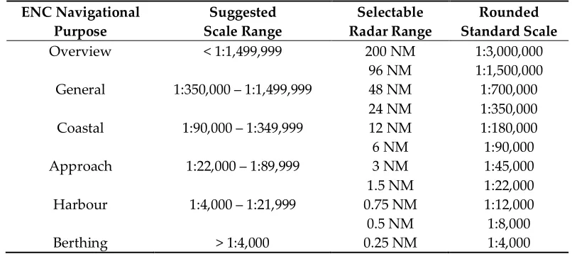
contingent user considerations and, as such, difficult to be estimated. Together with the degree of
67
interpolation bias, the likely existence of a few special cases related to the presence of feature types
68
like marine farms, restricted areas, and other types of obstructions complicates the identification of
69
discrepancies between nautical charts and the survey soundings [12].
70
The evaluation of current chart adequacy (as well as the rectification of possible deficiencies and
71
shortcomings) represents a world-wide pressing need that poses a challenge to many national
72
hydrographic offices [13,14]. Those offices must balance such a pressing need with the limited
73
available resources and survey priorities that translate to the fact that decades may past until a new
74
hydrographic survey can be conducted in a given area. In such an optic, it is becoming more and
75
more obvious the requirement to evaluate the adequacy of the chart portfolio not only using newly
76
collected bathymetric sonar bathymetry (BSB) but any possible source of geospatial information like
77
automatic-identification system (AIS) data or alternative surveying means like synthetic aperture
78
radar (SAR) shoreline extraction, satellite derived bathymetry (SDB) and airborne-lidar bathymetry
79
(ALB)[6,14-20]. However, given the physically-limited penetration in water of SAR, SDB and ALB as
80
well as the circular limitation in retrieving information from AIS data (i.e., vessels tend to avoid
81
uncharted areas), BSB surveys – despite their high cost and logistic challenges – not only provide
82
both highly accurate and dense measurements of the seafloor morphology, but also represent the
83
only practical source of hydrographic information for large parts of the ocean [15].
84
The identification of nautical chart discrepancies in comparison to newly collected hydrographic
85
survey datasets has received only limited attention in the scientific literature despite its importance
86
for the safety of navigation and relevance in the evaluation of the adequacy of the current charts, as
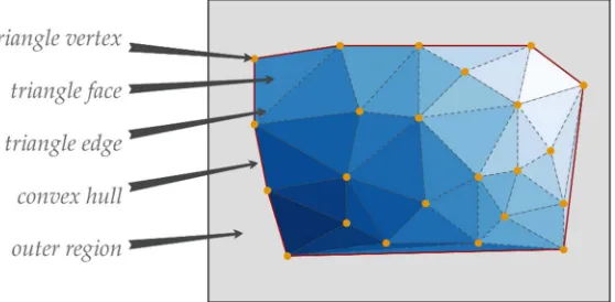
87
well as for coastal change analysis and coastal zone management [21-25]. In addition, many of the
88
techniques developed for geospatial data analysis on land cannot be straightly applied to the nautical
89
cartography realm, mainly because of the peculiar safety of navigation requirement [12,26-29].
90
Currently, the task to identify chart discrepancies against new BSB data sets is usually performed by
91
the various cartographic agencies through manual or semi-automated processes, based on best
92
practices developed over the years. However, these processes require a substantial level of human
93
commitment that includes the visual comparison of the chart against the new data, the analysis of
94
intermediate support products or, more commonly, a combination of the two.
95
This work describes an algorithm that aims to automate a large extent of the change detection
96
process and to reduce its subjective human component. Through the selective derivation of a set of
97
preliminary tilted-triangle test to all the input survey soundings. Given the complexity of a modern
99
nautical chart, a set of additional sounding-in-specific-feature tests are then performed. As output,
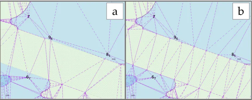
100
the algorithm provides DtoN candidates, chart discrepancies (the “deep” discrepancies may be
101
optionally identified), and a subset of features that requires human evaluation (if any). The algorithm
102
has been successfully tested with real-world Electronic Navigational Charts (ENCs) and survey
103
datasets. In parallel to the development of this work, an application implementing the algorithm was
104
created and made publicly available in the HydrOffice framework
105
(https://www.hydroffice.org/catools).
106
2. Materials and Methods
107
2.1. Electronic Navigational Charts
108
An ENC provides all the information for safe navigation in the form of a database – standardized
109
as to content, structure and format – issued on the authority of government authorized hydrographic
110
offices [30]. As such, it does not only contain information for safe navigation present in the
111
corresponding paper chart but can embed supplementary material present in other kinds of nautical
112
publications (e.g., sailing directions). The ENC content may be directly derived from original survey
113
material, but also from databased information, existing paper charts or a combination of them [31].
114
The International Hydrographic Organization (IHO) has created a standard vector format,
115
named S-57, for official ENCs (that is, produced by a government hydrographic office) that contain a
116
set of data layers for a range of hydrographic applications. However, an IHO S-57 ENC is mainly
117
used, in combination with positional information from navigation sensors and radar data, by an
118
Electronic Chart Display and Information System (ECDIS) to provide a graphical representation of a
119
marine area, including bathymetry and topography, and to assist the mariner in route planning and
120
monitoring by providing natural features, man-made structures, coastlines, and any other
121
information related to marine navigation [6,32]. To meet high standards of reliability and
122
performance, an extensive body of rules defines an ECDIS with the result that, under SOLAS Chapter
123
V regulations, an ECDIS loaded with official ENCs is currently the only alternative for the navigator
124
to the adequate and up-to-date paper charts [33].
125
As defined by the IHO standard, the S-57 data content consists of a set of features that may have
126
a spatial representation in the form of points, lines or polygons. Based on the ENC product
127
specifications, those features must be encoded using the chain-node topology (Figure 1) [32,34]. For
128
a S-57 ENC, the basic unit of geographic coverage is called “cell”, normally a spherical rectangle
129
bordered by meridians and latitudes with actual data coverage of any shape [31]. Within the same
130
navigational purpose (e.g., coastal, approach) (Table 1), the cell data may not overlap with those of
131
the adjacent cells. The navigational purpose also drives the compilation scale and, thus, the features
132
134
Figure 1. Graphical representation of the chain-node topologic model enforced by the S-57 ENC
135
specifications. A geospatial feature may be represented as a point (by an isolated node), a line (using
136
a series of edges and connected nodes), or an area (by a closing loop of edges starting and ending at
137
a common connected node). Vector objects may be shared, but duplication of coincident linear
138
geometry is prohibited [32].
139
Table 1. The ENC navigational purposes with range of compilation scales (and the standard radar
140
scale within each range) suggested by the IHO S-65 publication [31].
141
ENC Navigational Purpose
Suggested Scale Range
Selectable Radar Range
Rounded Standard Scale
Overview < 1:1,499,999 200 NM 1:3,000,000
96 NM 1:1,500,000 General 1:350,000 – 1:1,499,999 48 NM 1:700,000
24 NM 1:350,000
Coastal 1:90,000 – 1:349,999 12 NM 1:180,000
6 NM 1:90,000
Approach 1:22,000 – 1:89,999 3 NM 1:45,000
1.5 NM 1:22,000
Harbour 1:4,000 – 1:21,999 0.75 NM 1:12,000
0.5 NM 1:8,000
Berthing > 1:4,000 0.25 NM 1:4,000
142
2.2. Soundings from Bathymetric Sonar Surveys
143
In the hydrographic field, a sounding can be intended as a measured depth of water (i.e., a
144
survey sounding) or as a bathymetric value represented on a nautical chart (i.e., a charted sounding)
145
[30]. The algorithm described in this work digests both kinds of soundings, but with distinct uses. In
146
fact, the survey soundings collected using bathymetric sonars – with multibeam sonars (MBES)
147
currently playing a predominant role as acquisition devices – are analyzed as proxies for the
bathy-148
morphology of the surveyed area [35], while the charted soundings represent one of the many feature
149
types retrieved from the ENC to reconstruct the bathymetric model that the nautical cartographer
150
wanted to communicate at the time of the ENC compilation (and, when present, after the application
151
The algorithm described in this work was developed to handle as input the following types of
153
survey soundings:
154
“Pure survey soundings”, intended as the point cloud measured by a bathymetric sonar after
155
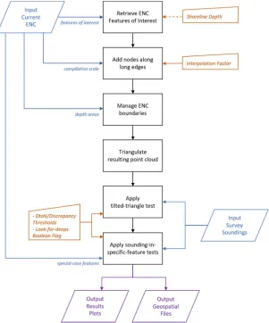
having been properly integrated with ancillary sensors, cleaned by spurious measurements and
156
reduced to the chart datum.
157
“Gridded survey soundings”, represented by the nodes with valid depth values in a
regularly-158
spaced grid created using the pure survey soundings.
159
“Selected gridded survey soundings”, commonly generated during the cartographic processing
160
using algorithms that select the grid nodes that are more meaningful to depict the trend of the
161
underlining bathymetric model.
162
Assuming the correctness in the generation of the above three types of survey soundings (whose
163
evaluation is outside of the scope of the present work), the algorithm provides similar output results,
164
with the only relevant difference of the number of flagged features. The latter is justified by the
165
different number of survey soundings in input: the gridding and the selection processes commonly
166
reduce the amount of features input of one or more orders of magnitude.
167
2.3. Bathymetric Model Reconstruction using a Triangulated Irregular Network (TIN)
168
From a general point of view, a TIN consists of a network of irregular triangles generated by
169
connecting the nodes of a dataset in a way that guarantees the absence of intersecting triangle edges
170
and superposed triangle faces, but also that the union of all the triangles fills up the convex hull of
171
the triangulation (see Figure 2) [36]. For the aims of this work, we generate a TIN from a set of
three-172
dimensional nodes retrieved from the chart and then assume a linear variation of the bathymetric
173
model among those nodes.
174
175
Figure 2. Example of a Triangulated Irregular Network (TIN) with the adopted nomenclature for the
176
various components.
177
The generated TIN is based on the Delaunay conforming triangulation [37] selected for the
well-178
known characteristic properties (e.g., being mathematically well defined, providing an unique output
179
for a given dataset independently from the data sequence) [38]. In the literature, several algorithms
180
implementing such a triangulation are available [39,40]. For the present work, we adopted the
181
practical convex hull algorithm that combines the two-dimensional Quickhull algorithm with the
182
general-dimension Beneath-Beyond algorithm, using the implementation provided by the open
183
source QHull code library [41].
184
For the bathymetric model reconstruction, the algorithm retrieves nodes from the following
185
ENC feature types (in parenthesis, the adopted S-57 acronym):
186
Charted soundings (SOUNDG).
187
Depth contour lines (DEPCNT) with a valid depth value attribute (VALDCO).
188
Dredged area polygons (DRGARE) with a valid value for the minimum deptnh range attribute
189
(DRVAL1).
190
All the point features with a valid value of sounding attribute (VALSOU).
191
Depth area polygons (DEPARE) for the ENC cell boundaries only.
193
To avoid the creation of triangles crossing feature edges (and, thus, the corresponding
194
misrepresentation in the reconstructed bathymetric model), additional nodes are inserted along the
195
feature edges that are longer than the interpolation length ( ) of one centimeter ( = 0.01 ) at
196
the ENC compilation scale ( ) (Figure 3):
197
= . (1)
For example, with a value of 1:10,000, the obtained by applying (1) is 100 meters. Given
198
that the position of features in an ENC are provided in geographic coordinates referred to the World
199
Geodetic System 1984 Datum (WGS84), the metrical value is then converted to its corresponding
200
geographic value using the local latitude [31,32].
201
The algorithm retrieves the for (1) directly from the ENC, using the value stored in the
202
“Compilation Scale of Data” (S-57 label: CSCL) subfield in the “Data Set Parameter” (S-57 field tag:
203
DSPM) field structure [32]. By definition, such a value represents the compilation scale appropriate
204
to the greater part of the data in the cell [32]. The derivation of the interpolation factor, , from the
205
ENC analysis (i.e., by looking at the distribution of the distance among the features) was attempted,
206
but it did not provide satisfying results, mainly because of the intrinsic variable-resolution nature of
207
a nautical chart. The one-centimeter interpolation value was then established heuristically as a
trade-208
off value between the requirement of avoiding the triangle-crossing-edge condition and the
209
performance cost paid for a larger point cloud to triangulate. The effectiveness of has been
210
empirically tested using real-world ENCs, but more conservative values for – or its derivation
211
from more advanced ENC analysis (e.g., locally estimating rather than attempting to define a
212
single value for the full chart) – may be adopted.
213
214
Figure 3. Pane (a) shows an example retrieved from an ENC where the long sides of a dredged-area
215
feature (visualized with a dotted pattern) trigger the creation of triangles (dashed magenta lines) that
216
overlap with the same feature edges. After the application of the proposed interpolation criterion, the
217
resulting triangulation shown in pane (b) does not present the overlap issue.
218
In addition to the described point densification, the reconstruction of a bathymetric model from
219
an ENC requires to associate a depth value to the nodes derived from the shoreline features, and that
220
such a value is referenced to the chart vertical datum like all the other depth nodes. Given that chart
221
producers may adopt different methods to identify the shoreline, the algorithm takes the depth value
222
for the shoreline as an input parameter. However, if not provided, the algorithm defaults to use the
223
shallowest depth value among all the valid depth values in the collected nodes.
224
The boundaries of the ENC bathymetry may be defined by the shoreline features and by the cell
225
data limits. In this latter case, based on the enforced chain-node topology, the algorithm retrieves the
226
nodes delimiting the point cloud by intersecting the depth area polygons along the cell boundaries
227
range attribute (S-57 acronym: DRVAL1). In the rare cases where such a value is not populated in the
229
input ENC, the reconstruction of the bathymetric model along those edges cannot be performed and,
230
thus, the evaluation of any survey sounding present in these ambiguous areas is delegated to the
231
analyst.
232
2.4. Application of the Tilted-Triangle Test
233
Once the TIN has been generated, the input survey soundings are categorized after the
234
identification of the containing triangle. If a specific survey sounding is outside of all the TIN triangles
235
or is contained within a triangle with all the vertices having the same value (hereinafter referred to
236
as a “flat triangle”), the algorithm temporarily stages it for being re-examined in the step described
237
in the following section.
238
When an input sounding, , is within a TIN triangle, the algorithm calculates the equation of
239
the tilted plane, ( , , ), containing the three triangle vertices, , , :
240
+ + + = 0 (2)
where:
241
= −− −− ,
= −− −− ,
= −− −− , and
= −( + + ).
The normal for such a tilted plane can be calculated as:
242
= + + . (5)
The vertical line containing the point can be expressed in its parametric form, using for the
243
position vector and the line verticality for identifying the direction vector :
244
= + (3)
where the scalar varies to identify all the possible infinite point belonging to the vertical line.
245
After having identified both the vertical line passing for the sounding and the tilted plan, the
246
algorithm identifies the intersection point between the two geometrical entities by calculating
247
using [42]:
248
=−( ⋅ + )
⋅ (4)
The vertical distance, Δ , is calculated as the difference between the depth dimensions between
249
the sounding, , and its vertical interception point with the tilted plan, :
250
Δz = − . (6)
The algorithm uses the Δz to evaluate whether flagging the soundings as DtoN candidates
251
(Figure 4) or potential chart discrepancies. The default logic of the applied thresholding (Table 2) is
252
derived from the NOAA Office of Coast Survey (OCS) Hydrographic Surveys Specifications and
253
Deliverables (HSSD) manual [43]. In deep waters, the DtoN concept does not apply to surface
254
navigation. However, based on the consideration that the presence of a very large discrepancy in
255
comparison to the charted water depth may represent an issue for specific marine operations (e.g.,
256
towing a side scan sonar), the algorithm reports – when using default parameters – potential DtoNs
257
for Δz values larger than the ten percent of the water depth. However, since those values should
258
follow the specific policy (or other types of specific needs) of the adopting cartographic organization,
259
while the current ones are inspired by best practices in [43], the algorithm was made flexible to accept
260
262
Figure 4. An example of DtoN detection. In the pane (a), a 10.1-meter survey sounding (in blue) is
263
surrounded by two charted soundings (in black) and two depth contours of ten meters and twenty
264
meters. The pane (b) shows the result of the triangulation (dashed lines in magenta) and a DtoN
265
candidate (grey circle with a cross simple). This latter has a vertical distance of about five meters (red
266
value overlaying the circle) from the underlying tilted triangle.
267
268
Table 2. Default threshold values adopted by the algorithm to identify the DtoN candidates and
269
potential chart discrepancies. For depth values less than 20 meters, the adopted threshold follows best
270
practices defined in the NOAA OCS HSSD manual [42]. Deeper waters have a much less compelling
271
safety-of-navigation requirement; thus, the chosen percentages of water depth were selected after
272
having considered the required IHO standard requirements for the original survey data. Adopting
273
cartographic agencies should modify such values based on their adopted best practices.
274
Threshold type z < 20 meters z >= 20meters
Danger to Navigation 1.0 meter 10.0 % of water depth
Chart Discrepancy 0.5 meter 5.0 % of water depth
275
Although large negative Δz values (“deeps”) do not represent a concern from a safety of
276
navigation perspective, their presence provides evidence of chart inconsistencies. As such, the
277
algorithm can be optionally set to identify those deeps, by simply applying a reversed thresholding
278
logic in respect to the “shallow” chart discrepancies.
279
2.5. Application of the Sounding-in-Specific-Feature Tests
280
Due to the complexity of a modern nautical chart, the tilted-triangle test alone is not sufficient
281
to properly evaluate all the possible feature configurations that can be depicted on an ENC. As such,
282
the algorithm complements the described in paragraph 2.4 with a set of additional
sounding-in-283
specific-feature tests.
284
From a geometrical point of view, the first common operation of such tests is to check whether
285
a given sounding point is inside any of the polygons that belong to a specific feature type.
286
Computationally, the detection of the presence of a point inside a polygon is most commonly done
287
using the Ray Casting algorithm [44,45]. Among the several existing implementations available to
288
assess topological relationship between geospatial objects, the algorithm adopted the vectorized
289
binary predicates provided by the Shapely library [46].
290
A common use case of the point-in-polygon test is provided by the mentioned possible presence
291
of a survey sounding within a flat TIN triangle. A flat triangle can be generated as the result of the
292
triangulation in areas locally characterized by the presence of a linear feature – like a curved depth
293
algorithm compares the given survey sounding against the validity depth range – when available –
295
of the underlying feature polygon (e.g., a depth area).
296
297
Figure 5. An example of presence of a survey sounding in a flat triangle. In the pane (a), an 8.3-meter
298
survey sounding (in blue) is surrounded by the nodes of a 10-meter depth contour that are closer than
299
the charted soundings (in black). As such, the survey sounding will be contained by a flat triangle
300
(that is, with three vertices having a 10-meter depth) shown in magenta in the pane (b). By adopting
301
the sounding-in-specific-feature test, the algorithm flagged the survey sounding as a potential
302
discrepancy (shown as grey circle with a depth difference of 1.7 meters in red) since it was detected
303
as contained by a depth area with a valid depth range between ten and twenty meters.
304
The S-57 ENC specifications prescribe that a cell must have the entire area with data covered,
305
without any overlap, by a restricted group of seven area feature types, called the “skin of the earth”
306
(Table 3) [32]. This characteristic of a S-57 ENC contributes to make the sounding-in-specific-feature
307
tests effective to reduce the number of staged untested features. Furthermore, if a survey sounding
308
is not contained in any of the skin of the earth polygons, it is outside of the ENC data coverage and
309
thus does not represent a chart discrepancy.
310
Table 3. The S-57 ENC area feature types, with the corresponding acronym, belonging to the restricted
311
“skin of the earth” group.
312
Feature Type S-57 Acronym
Navigable depth areas DEPARE
Dredged area DRGARE
Floating dock FLODOC
Permanently moored ship HULKES
Land area LNDARE
Pontoon PONTON
Unsurveyed depth area UNSARE
313
314
Figure 6 provides a flowchart outlining the main algorithmic steps, data inputs, user parameters,
315
and processing outputs. The plots provided in output should only be used for exploratory means. In
316
fact, once that the algorithm is successfully executed, the generated geospatial files should be
317
imported in the full-fledged GIS application of choice for results inspection and eventual application
318
320
Figure 6. The flowchart shows, in black, the main steps of the proposed algorithm. The inputs are
321
represented in blue, the user parameters in orange (with a dashed connector when optional), and the
322
outputs in purple.
323
2.6. Library Implementation, Supporting Visualization, and Output Storage
324
A software library (current version: 1.0) that implements the algorithm has been developed and
325
tested mostly using the Python language (version 3.6) [47]. For a few selected profiled bottlenecks, a
326
superset of Python, called Cython (version 0.28) [48], was used to reduce the execution time by
327
manually adding a few static type declarations. Using such declarations, Cython was then able to
328
automatically convert Python code into optimized C code.
329
The library has been coupled with a multi-tab graphical user interface based on a Python port
330
of the Qt framework [49]. The outcomes of the algorithm execution are visualized using the
331
Matplotlib library [50]. ENC-derived depth values are colored by depth, while algorithm-flagged
332
input survey soundings are colored by their discrepancy. If present, the subset of untested input
333
soundings that require human evaluation are displayed with a magenta diamond. The default output
334
is provided in S-57 format using internal code. For easy sorting and identification of discrepancies,
335
the magnitude of the discrepancy against the chart is stored both as cartographic symbol features
(S-336
57 acronym: $CSYMB) and soundings (i.e., storing the discrepancy value as the depth coordinate).
337
Optional output in the popular Shapefile and KML formats are generated using the Geospatial
338
Data Abstraction Library (GDAL) package [51]. In this latter case, the TIN internally used by the
339
algorithm is also generated for debugging aims. An implementation of the algorithm was made
340
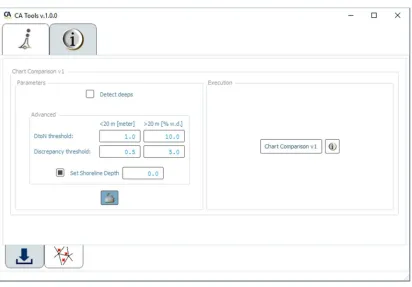
publicly available in the HydrOffice framework as a tab widget (Figure 7) freely accessible in the CA
341
343
Figure 7. Screenshot of the tab widget present in the HydrOffice CA Tools application. The widget
344
exposes, on the left area, some of the algorithm parameters.
345
3. Results
346
At the best of our knowledge, the literature currently lacks algorithms specifically tailored to the
347
identification of discrepancies between nautical charts and survey soundings and, thus, with
348
outcomes directly comparable with the proposed algorithm. However, the algorithm results were
349
quantitatively compared, only for the DtoNs component, with the output of a tool named DtoN
350
Scanner (version 2) described in [25] and publicly available as part of the HydrOffice QC Tools
351
application (https://www.hydroffice.org/qctools/main). All the algorithm results were also validated
352
based on expert opinion.
353
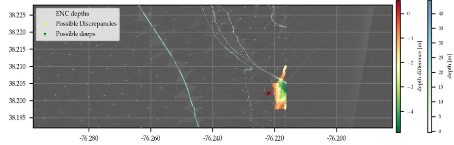
During the initial development, ad-hoc input survey soundings have been generated with two
354
DtoNs and two chart discrepancies to be tested against a valid ENC. Using the described default
355
settings, the algorithm was able to identify both the DtoNs and the chart discrepancies Figure 8.
356
357
Figure 8. Algorithm results when applied to the ad-hoc input survey soundings. The possible DtoN
358
are presented using cross markers, while triangular markers are used for the possible discrepancies.
359
The nodes are represented as dots, with the connecting triangle edges in gray. Axes in geographical
360
The algorithm has then been tested in several real-data scenarios using official ENCs and
MBES-362
based survey datasets. To keep this section concise, only two of those scenarios are here presented.
363
On one side, the analysis of the soundings from NOAA survey H12990 (see Figure 9) shows relatively
364
minor changes to the current ENCs. Conversely, the presence of large active glaciers in the area is
365
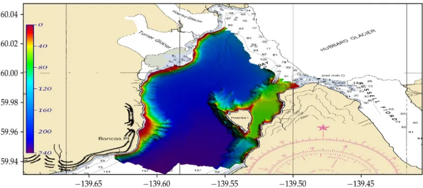
highlighted by the analysis of the NOAA H13701 dataset. Further details of the adopted inputs are
366
provided, for the surveys, in Table 4 and, for the ENCs, in Table 5.
367
368
Figure 9. Bathymetric model generated using the data collected by the NOAA H12990 survey. The
369
NOAA raster nautical charts 12331 (Chesapeake Bay Tangier Sound Northern Part) and 12333
370
(Potomac River Chesapeake Bay to Piney Point) are shown in the background. Bathymetric values in
371
the color bar (in blues) are in meters and referred to the MLLW vertical datum. Axes in geographical
372
WGS84 coordinates.
373
374
Figure 10. Bathymetric model generated using the data collected by the NOAA H13071 survey. The
375
NOAA raster nautical charts 16761 (Yakutat Bay) is shown in the background. Bathymetric values in
376
the color bar (in blue) are in meters and referred to the MLLW vertical datum. Axes in geographical
377
WGS84 coordinates.
378
Table 4. Information about the NOAA surveys presented as test datasets.
380
Survey Location Year Scale MBES
H12990 Chesapeake Bay (USA) 2017 1:10,000 Kongsberg EM 2040
H13071 Yakutat Bay (USA) 2017 1:40,000 Kongsberg EM 710, Kongsberg EM 2040
Table 5. Information about the NOAA ENCs used to test the algorithm.
381
Chart Scale Edition Update Number Issue Date
US5VA21M 1:40,000 21 0 2 May 2018
US5VA22M 1:40,000 28 2 5 June 2018
US4AK3XM 1:80,000 5 0 13 February 2018
382
The results of the analysis for the H12990 survey dataset are shown in Figure 11 and Figure 12.
383
These two figures represent the evaluation of the westernmost and easternmost parts, respectively of
384
the survey that insists in two different ENCs.
385
386
Figure 11. Algorithm results using the western part of the H12990 survey soundings compared to the
387
US5VA21M ENC. Axes in geographical WGS84 coordinates.
388
389
Figure 12. Algorithm results using the eastern part of the H12990 survey soundings compared to the
390
US5VA22M ENC. Axes in geographical WGS84 coordinates.
391
393
Figure 13. Algorithm results using the H13701 survey soundings compared to the US4AK3XM ENC.
394
Axes in geographical WGS84 coordinates.
395
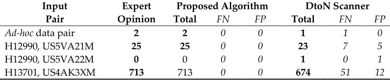
The three applied analyses to the two presented surveys provide results that are consistent with
396
what reported by survey analysts – using their judgement to evaluate the context surrounding the
397
survey sounding, but with numeric criteria adherent to Table 2 – after a careful but time-consuming
398
evaluation of the same inputs (see Table 6, for DtoN candidates, and Table 7, for chart discrepancies).
399
The comparison with the expert opinion identified the presence of a few false positives (Table 7)
400
mainly localized close to the ENC boundaries. This is not surprising given the currently adopted
401
approach of using the minimum value in depth areas along the ENC boundaries for introducing
402
additional nodes. A possible future improvement to mitigate such an issue is the merge of point
403
clouds retrieved from adjacent ENCs – at the same navigational purpose – before performing the
404
“Triangulate resulting point cloud” step (Figure 6).
405
For the DtoNs candidates, the proposed algorithm performed better than the DtoN Scanner in
406
terms of both false negatives and false positives. The better performance can be reconducted to the
407
adoption of more capable tests (the DtoN Scanner only uses a “flat” triangle test with the shallowest
408
depth of each triangle vertices) and the additional techniques adopted during the construction of the
409
point cloud from the ENC (e.g., the long-edge interpolation, the adoption of a proper shoreline depth
410
value, the retrieval of the ENC boundaries).
411
Table 6. Results for DtoN candidates using the proposed algorithm and the DtoN Scanner [25]. The
412
Expert Opinion column provides the total number of DtoNs used to identify the false negatives (FN)
413
and the false positives (FP) for the two sets of automated outputs.
414
Input Pair
Expert Opinion
Proposed Algorithm DtoN Scanner
Total FN FP Total FN FP
Ad-hoc data pair 2 2 0 0 1 1 0
H12990, US5VA21M 25 25 0 0 23 7 5
H12990, US5VA22M 0 0 0 0 1 0 1
H13701, US4AK3XM 713 713 0 0 674 51 12
Table 7. Results for chart discrepancies using the proposed algorithm. The Expert Opinion column
416
provides the total number of chart discrepancies used to identify the false negatives (FN) and the false
417
positives (FP) for the automated output.
418
Input Pair
Expert Opinion
Proposed Algorithm Total FN FP
Ad-hoc data pair 2 2 0 0
H12990, US5VA21M 107 110 0 3
H12990, US5VA22M 2 3 0 1
H13701, US4AK3XM 779 784 0 5
419
4. Discussion
420
Although the algorithm has been successfully tested with several pairs of real-world ENCs and
421
survey datasets, more tests are required to identify possible shortcomings and corner cases absent in
422
the analyzed scenarios. However, the handling of eventual issues will likely happen by extending the
423
described two-step approach and, thus, preserve the general validity of the algorithm proposed in
424
this work.
425
Although popular, the IHO S-57 ENC format is not the only available format to store the
426
geospatial vector information of a nautical chart for use with an ECDIS (e.g., the National Geospatial
427
Agency’s Digital Nautical Chart format, the coming IHO S-101 standard) [33,52]. Although this work
428
is based only on ENC data in the IHO S-57 format, the extension to other ENC formats should be
429
straightforward.
430
The survey soundings are ultimately limited by the quality of the original observations used to
431
sample the seafloor [53]. This consideration acquires increasing relevance when the dimensions of
432
the measured chart discrepancies approaches the limits – that should be experimentally evaluated or
433
retrieved by the specifications declared by the manufacturer – of the sonar system used for the survey
434
[54]. The sonar detection uncertainty represents just one potential source of artifacts with a variety of
435
other potential environmental, integration and datum reduction issues that can badly affect the final
436
survey soundings [35,55]. When this happens, bathymetric artifacts generated by the acoustic
437
imaging geometry may be mistaken as chart discrepancies. Among other institutions, the
438
International Hydrographic Organization has developed rules and best practices for the execution of
439
a hydrographic survey that fulfills minimum quality requirements for charting aims [56,57].
440
However, the execution of a hydrographic survey is not always targeted at the production of nautical
441
charts. New hydrographic data are collected for a variety of reasons that spans from scientific
442
research to military applications and marine constructions [58]. Given the high cost of data collection
443
at sea, the national hydrographic offices usually attempt to use those surveys, when made them
444
available, for charting purposes. As such, a buffer representing a lower limit of what is considered a
445
chart discrepancy should also consider an estimation of the soundings quality based on the specific
446
survey being analyzed.
447
A preliminary step in the application of the algorithm consists in the retrieval of the information
448
content present in the input ENC. Ideally, such a content should be used to reconstruct a continuous
449
bathymetric model of the ENC’s underwater area that matches – as close as possible – the intent of
450
the chart makers and the expectations of the chart readers. In practice, it is unlikely that, based on
451
different precautionary principles and contingent valuations, two random navigators would draw a
452
perfectly overlapping intermediate contour on a given ENC area. Given the complexity and inherent
453
subjectivity involved in the bathymetric reconstruction, we opted for a simplified, still reasonable
454
solution for the task by generating a TIN from the set of three-dimensional nodes retrieved from the
455
chart and then assuming a linear variation of the model among those nodes.
456
In alternative to the use of the Delaunay conforming triangulation, future works may explore
457
the creation of the TIN based on a constrained Delaunay triangulation [59,60], since this technique
458
makes possible to explicitly define edges (“breaklines”) that are not modified by the triangulator
459
the adopted point densification for long feature edges provides a controlled mean to introduce nodes
461
in the triangulation. Thus, we will likely also explore the adoption of a hybrid solution.
462
The conversion by interpolation of a TIN into a regular grid to perform discrepancy analysis
463
represents a quite popular operation. However, although the several intrinsic advantages related to
464
deal with grid data (e.g., higher processing and development speed) [36], we decided to not take such
465
a direction because of the intrinsic variable-resolution nature of an ENC that makes difficult to
466
identify the best fixed resolution at which to grid the TIN. Regarding the possible creation of a
467
variable-resolution grid, despite the recent development and successful application of this type of
468
gridding algorithms to MBES data [61], a robust estimation of the local resolution based on a
ENC-469
derived data would have represented a challenge, and it is an open research question.
470
At the best of our knowledge, this work represents the first appearance in literature of a
471
proposed algorithm for identifying discrepancies between nautical charts and survey soundings.
472
Thus, there is a lack of research efforts that the results of this work can be directly compared with,
473
with the notable exception of the DtoN Scanner [25]. However, the described tilted-triangle test may
474
be seen as an evolution of a well-known best practice in nautical cartography for the representation
475
of depth during chart compilation [21]. Such a practice, known as the “triangular method of selection”
476
[62], is commonly used to drive the selection of the charted soundings, and it is based on the following
477
two tests:
478
Triangle test. Within a triangle of charted soundings, no survey sounding is present which is
479
less than the shallowest depth values defining the corners of the triangle.
480
Edge test. Between two adjacent charted soundings, no survey sounding exists shallower than
481
the lesser of the two charted soundings.
482
The application of those tests presents some well-known scale- and data density-dependent
483
issues (e.g., which spatial buffer to apply for the edge test? What is the significance of the triangle test
484
with narrow elongated triangles?) that the tilted-triangle test potentially overcomes.
485
5. Conclusions
486
The present work provides evidence that, with respect to chart adequacy assessment, the
487
adoption of the described two-step algorithm brings several improvements (e.g., less subjectivity and
488
time of execution) in comparison to the current commonly-adopted practices.
489
Future works will focus on exploring techniques to better reconstruct the bathymetric model
490
from ENCs (i.e., attempting to better capture the cartographer and the mariner interpretations of the
491
charted bathymetry) and evaluating the adaptation of the algorithm to chart compilation aims as a
492
replacement of the triangle test and the edge test.
493
494
Author Contributions: Methodology and data curation: G.M., T.F. and C.K.; software and visualization: G.M.;
495
formal analysis: G.M. and C.K.; validation, investigation, and resources: T.F.; writing—original draft
496
preparation: G.M.; writing—review and editing: T.F. and C.K.
497
Funding: This research was partially funded by the NOAA grant NA15NOS4000200.
498
Acknowledgments: Authors would like to thank the NOAA National Ocean Service (NOS) Office of Coast
499
Survey (OCS) and the Canadian Hydrographic Service (CHS) for the datasets, Mathieu Rondeau (CHS
500
Waterways Surveys Unit), Claude Tremblay (CHS Maurice Lamontagne Institute), and Peter Holmberg (NOAA
501
NOS Office of Coast Survey, Pacific Hydrographic Branch) for their support. Authors are also grateful to the
502
anonymous reviewers whose comments helped to improve the paper.
503
Conflicts of Interest: The authors declare no conflict of interest.
504
References
505
1. Russom, D.; Halliwell, H. Some Basic Principles in the Complication of Nautical Charts. The International
506
2. Mayer, L.; Jakobsson, M.; Allen, G.; Dorschel, B.; Falconer, R.; Ferrini, V.; Lamarche, G.; Snaith, H.;
508
Weatherall, P. The Nippon Foundation—GEBCO Seabed 2030 Project: The Quest to See the World’s Oceans
509
Completely Mapped by 2030. Geosciences 2018, 8, 63, https://doi.org/10.3390/geosciences8020063.
510
3. Pasquay, J.-N. Safety of modern shipping and requirements in hydrographic surveying and nautical
511
charting. The International Hydrographic Review 1986, 63.
512
4. Buixadé Farré, A.; Stephenson, S.R.; Chen, L.; Czub, M.; Dai, Y.; Demchev, D.; Efimov, Y.; Graczyk, P.;
513
Grythe, H.; Keil, K., et al. Commercial Arctic shipping through the Northeast Passage: routes, resources,
514
governance, technology, and infrastructure. Polar Geography 2014, 37, 298-324,
515
https://doi.org/10.1080/1088937X.2014.965769.
516
5. Masetti, G.; Calder, B. A Bayesian marine debris detector using existing hydrographic data products, OCEANS
517
2015 - Genova, 18-21 May 2015, 2015; pp 1-10, https://doi.org/10.1109/OCEANS-Genova.2015.7271584.
518
6. Roh, J.Y.; Shin, M.S.; Suh, Y.C.; Yang, I.T.; Lee, D.H. Evaluation of Nautical Chart Adequacy in the Coastal
519
Area around Incheon Bay using Satellite Imagery with AIS Data. Journal of Coastal Research 2017, 319-323,
520
https://doi.org/10.2112/SI79-065.1.
521
7. Moegling, C.; Holmberg, P. Journey of a Sounding: Application of NOAA Soundings and Features to Navigation
522
Products, U.S. Hydro Conference, New Orleans, LA, USA, 2013; New Orleans, LA, USA, p 17.
523
8. Calder, B.; Mayer, L. Automatic Processing of High-Rate, High-Density Multibeam Echosounder Data.
524
Geochemistry Geophysics And Geosystems 2003, 4, https://doi.org/10.1029/2002GC000486.
525
9. Shea, K.S.; McMaster, R.B. Cartographic generalization in a digital environment: When and how to generalize,
526
Proceedings Auto-Carto, 1989; pp 56-67.
527
10. Gökgöz, T.; Sen, A.; Memduhoglu, A.; Hacar, M. A New Algorithm for Cartographic Simplification of
528
Streams and Lakes Using Deviation Angles and Error Bands. ISPRS International Journal of Geo-Information
529
2015, 4, 2185, http://dx.doi.org/10.3390/ijgi4042185.
530
11. Tucci, M.; Giordano, A. Positional accuracy, positional uncertainty, and feature change detection in
531
historical maps: Results of an experiment. Computers, Environment and Urban Systems 2011, 35, 452-463,
532
https://doi.org/10.1016/j.compenvurbsys.2011.05.004.
533
12. James, L.A.; Hodgson, M.E.; Ghoshal, S.; Latiolais, M.M. Geomorphic change detection using historic maps
534
and DEM differencing: The temporal dimension of geospatial analysis. Geomorphology 2012, 137, 181-198,
535
https://doi.org/10.1016/j.geomorph.2010.10.039.
536
13. IHO. C-55: Status of Hydrographic Surveying and Charting Worldwide; Edition 31 July 2018; International
537
Hydrographic Organization: Monaco, 2018; p 528.
538
14. Klemm, A.; Pe'eri, S.; Freire, R.; Nyberg, J.; Smith, S.M. Nautical Chart Adequacy Evaluation Using
Publicly-539
Available Data, U.S. Hydro Conference, National Harbor, MA, USA, 2015; National Harbor, MA, USA, p 6.
540
15. Chénier, R.; Faucher, M.-A.; Ahola, R. Satellite-Derived Bathymetry for Improving Canadian
541
Hydrographic Service Charts. ISPRS International Journal of Geo-Information 2018, 7, 306,
542
https://doi.org/10.3390/ijgi7080306.
543
16. Lyzenga, D.R. Shallow-water bathymetry using combined lidar and passive multispectral scanner data.
544
International Journal of Remote Sensing 1985, 6, 115-125, https://doi.org/10.1080/01431168508948428.
545
17. Stumpf, R.P.; Holderied, K.; Sinclair, M. Determination of water depth with high-resolution satellite
546
imagery over variable bottom types. Limnology and Oceanography 2003, 48, 547-556,
547
https://doi.org/10.4319/lo.2003.48.1_part_2.0547.
548
18. Su, H.; Liu, H.; Heyman, W.D. Automated Derivation of Bathymetric Information from Multi-Spectral
549
Satellite Imagery Using a Non-Linear Inversion Model. Marine Geodesy 2008, 31, 281-298,
550
https://doi.org/10.1080/01490410802466652.
551
19. Pe’eri, S.; Parrish, C.; Azuike, C.; Alexander, L.; Armstrong, A. Satellite Remote Sensing as a
552
Reconnaissance Tool for Assessing Nautical Chart Adequacy and Completeness. Marine Geodesy 2014, 37,
553
293-314, https://doi.org/10.1080/01490419.2014.902880.
554
20. Pe'eri, S.; Madore, B.; Nyberg, J.; Snyder, L.; Parrish, C.; Smith, S. Identifying Bathymetric Differences over
555
Alaska's North Slope using a Satellite-derived Bathymetry Multi-temporal Approach. Journal of Coastal
556
Research 2016, 56-63, https://doi.org/10.2112/SI76-006.
557
21. Wilson, M.; Masetti, G.; Calder, B.R. Automated Tools to Improve the Ping-to-Chart Workflow.
558
International Hydrographic Review 2017, 17, 21-30.
559
22. Azuike, C.; Pe'eri, S.; Alexander, L.; Parrish, C.; Armstrong, A. Development of a Geo-spatial Analysis
560
Methodology for Assessing the Adequacy of Hydrographic Surveying and Nautical Charts, Canadian
561
Hydrographic Conference, Niagara Falls, Ontario, Canada, May 15 - May 17, 2012, 2012; Niagara Falls,
562
Ontario, Canada.
563
23. Moitoret, V.; Johnson, N.E. Automation of Hydrographic Source Data. The International Hydrographic Review
564
24. Furuya, H. Automating the Marine Chart Production Processes. Cartographica: The International Journal for
566
Geographic Information and Geovisualization 1973, 10, 23-36, https://doi.org/10.3138/6716-9222-4534-3440.
567
25. Wilson, M.; Masetti, G.; Calder, B. NOAA QC Tools: Origin, Development, and Future, Canadian
568
Hydrographic Conference, Halifax, Nova Scotia, Canada, 2016; Halifax, Nova Scotia, Canada.
569
26. Qi, H.B.; Li, Z.L.; Chen, J. Automated change detection for updating settlements at smaller-scale maps from
570
updated larger-scale maps. Journal of Spatial Science 2010, 55, 133-146,
571
https://doi.org/10.1080/14498596.2010.487855.
572
27. Armenakis, C.; Cyr, I.; Papanikolaou, E. Change detection methods for the revision of topographic
573
databases. Internatioanl Archives of Photogrammetry Remote Sensing and Spatial Information Sciences 2002, 34,
574
792-797.
575
28. Hussain, M.; Chen, D.; Cheng, A.; Wei, H.; Stanley, D. Change detection from remotely sensed images:
576
From pixel-based to object-based approaches. ISPRS Journal of Photogrammetry and Remote Sensing 2013, 80,
577
91-106, https://doi.org/10.1016/j.isprsjprs.2013.03.006.
578
29. Zhang, K.; Whitman, D.; Leatherman, S.; Robertson, W. Quantification of Beach Changes Caused by
579
Hurricane Floyd Along Florida's Atlantic Coast Using Airborne Laser Surveys. Journal of Coastal Research
580
2005, 123-134, https://doi.org/10.2112/02057.1.
581
30. IHO. S-32: Hydrographic Dictionary - English; International Hydrographic Bureau: Monaco, 1994;
582
http://hd.iho.int/en/index.php/Main_Page.
583
31. IHO. S-65: Electronic Navigational Charts (ENCs) “Production, Maintenance and Distribution Guidance"; Edition
584
2.1.0; International Hydrographic Organization: Monaco, 2017.
585
32. IHO. S-57: Transfer standard for digital hydrographic data; Edition 3.1; International Hydrographic
586
Organization: Monaco, 2000.
587
33. Alexander, L. Electronic Charts. In The American Practical Navigator, National Imaging and Mapping
588
Agency: Bethesda, MD, USA, 2003; pp 199-215.
589
34. Theobald, D.M. Topology revisited: representing spatial relations. International Journal of Geographical
590
Information Science 2001, 15, 689-705, https://doi.org/10.1080/13658810110074519.
591
35. Hughes Clarke, J.E. The Impact of Acoustic Imaging Geometry on the Fidelity of Seabed Bathymetric
592
Models. Geosciences 2018, 8, 109.
593
36. De Wulf, A.; Constales, D.; Stal, C.; Nuttens, T. Accuracy aspects of processing and filtering of multibeam data:
594
grid modeling versus TIN based modeling, FIG Working week, 2012; pp 6-10.
595
37. Delone, B. Sur la sphère vide. A la mémoire de Georges Voronoi. Bull. Acad. Sci. URSS. Cl. Sci. Math. 1934,
596
6, 793-800, http://mi.mathnet.ru/eng/izv4937.
597
38. Rebay, S. Efficient Unstructured Mesh Generation by Means of Delaunay Triangulation and
Bowyer-598
Watson Algorithm. Journal of Computational Physics 1993, 106, 125-138,
599
https://doi.org/10.1006/jcph.1993.1097.
600
39. Su, P.; Scot Drysdale, R.L. A comparison of sequential Delaunay triangulation algorithms. Computational
601
Geometry 1997, 7, 361-385, https://doi.org/10.1016/S0925-7721(96)00025-9.
602
40. Cheng, S.-W.; Dey, T.K.; Shewchuk, J. Algorithms for constructing Delaunay triangulations. In Delaunay
603
Mesh Generation, Chapman and Hall/CRC: 2016.
604
41. Barber, C.B.; Dobkin, D.P.; Huhdanpaa, H. The quickhull algorithm for convex hulls. ACM Trans. Math.
605
Softw. 1996, 22, 469-483, https://doi.org/10.1145/235815.235821.
606
42. Vince, J. Geometry for computer graphics: formulae, examples and proofs. Springer Science & Business Media:
607
2006; https://doi.org/10.1007/978-1-84628-997-2.
608
43. NOAA. Hydrographic Surveys Specifications and Deliverables; Edition April 2018; National Oceanic and
609
Atmospheric Administration, National Ocean Service: 2018; p 159.
610
44. Shimrat, M. Algorithm 112: Position of point relative to polygon. Commun. ACM 1962, 5, 434,
611
10.1145/368637.368653.
612
45. Haines, E. Point in polygon strategies. In Graphics gems IV, Paul, S.H., Ed. Academic Press Professional,
613
Inc.: 1994; pp 24-46.
614
46. Gillies, S.; Bierbaum, A.; Lautaportti, K.; Tonnhofer, O. Shapely: manipulation and analysis of geometric
615
objects. 2007; https://github.com/Toblerity/Shapely.
616
47. van Rossum, G. The Python Language Reference: Release 3.6.4. 12th Media Services: 2018; p 168.
617
48. Behnel, S.; Bradshaw, R.; Citro, C.; Dalcin, L.; Seljebotn, D.S.; Smith, K. Cython: The Best of Both Worlds.
618
Computing in Science and Engg. 2011, 13, 31-39, https://doi.org/10.1109/MCSE.2010.118.
619
49. The Qt Framework. https://www.qt.io/what-is-qt/ (August 2018).
620
50. Hunter, J.D. Matplotlib: A 2D Graphics Environment. Computing in Science & Engineering 2007, 9, 90-95,
621
51. Warmerdam, F. The Geospatial Data Abstraction Library. In Open Source Approaches in Spatial Data
623
Handling, Hall, G.B.; Leahy, M.G., Eds. Springer Berlin Heidelberg: Berlin, Heidelberg, 2008; pp 87-104,
624
https://doi.org/10.1007/978-3-540-74831-1_5.
625
52. IHO. S-101 Value Added Roadmatp; Edition April 2016; International Hydrographic Organization: 2016.
626
53. Hughes Clarke, J.E. Multibeam Echosounders. In Submarine Geomorphology, Micallef, A.; Krastel, S.; Savini,
627
A., Eds. Springer International Publishing: Cham, 2018; pp 25-41,
https://doi.org/10.1007/978-3-319-57852-628
1_3.
629
54. Lurton, X.; Augustin, J.M. A Measurement Quality Factor for Swath Bathymetry Sounders. IEEE Journal of
630
Oceanic Engineering 2010, 35, 852-862, https://doi.org/10.1109/JOE.2010.2064391.
631
55. Masetti, G.; Kelley, J.G.W.; Johnson, P.; Beaudoin, J. A Ray-Tracing Uncertainty Estimation Tool for Ocean
632
Mapping. IEEE Access 2018, 6, 2136-2144, https://doi.org/10.1109/ACCESS.2017.2781801.
633
56. IHO. S-44: Standards for Hydrographic Surveys; Edition 5; International Hydrographic Organization:
634
Monaco, 2008.
635
57. IHO. C-13: Manual Of Hydrography; Edition 1.04; International Hydrographic Organization: Monaco, 2011.
636
58. Kastrisios, C.; Pilikou, M. Nautical cartography competences and their effect to the realisation of a
637
worldwide Electronic Navigational Charts database, the performance of ECDIS and the fulfilment of IMO
638
chart carriage requirements. Marine Policy 2017, 75, 29-37, https://doi.org/10.1016/j.marpol.2016.10.007.
639
59. Paul Chew, L. Constrained delaunay triangulations. Algorithmica 1989, 4, 97-108,
640
https://doi.org/10.1007/BF01553881.
641
60. Hjelle, Ø.; Dæhlen, M. Constrained Delaunay Triangulation. In Triangulations and Applications, Springer
642
Berlin Heidelberg: Berlin, Heidelberg, 2006; pp 113-129, https://doi.org/10.1007/3-540-33261-8_6.
643
61. Calder, B.R.; Rice, G. Computationally efficient variable resolution depth estimation. Computers &
644
Geosciences 2017, 106, 49-59, https://doi.org/10.1016/j.cageo.2017.05.013.
645
62. IHO. S-4: Regulations of the IHO for International (INT) Charts and Chart Specifications of the IHO; Edition 4.6.0;
646
International Hydrographic Organization: Monaco, 2000.