c
Owned by the authors, published by EDP Sciences, 2015
The dynamic Virtual Fields Method on rubbers at medium and
high strain rates
Sung-Ho Yoonaand Clive R. Siviour
Department of Engineering Science, University of Oxford, Parks Road, Oxford, UK
Abstract. Elastomeric materials are widely used for energy absorption applications, often experiencing high strain rate deformations. The mechanical characterization of rubbers at high strain rates presents several experimental difficulties, especially associated with achieving adequate signal to noise ratio and static stress equilibrium, when using a conventional technique such as the split Hopkinson pressure bar. In the present study, these problems are avoided by using the dynamic Virtual Fields Method (VFM) in which acceleration fields, clearly generated by the non-equilibrium state, are utilized as a force measurement with in the frame work of the principle of virtual work equation. In this paper, two dynamic VFM based techniques are used to characterise an EPDM rubber. These are denoted as the linear and nonlinear VFM and are developed for (respectively) medium (drop-weight) and high (gas-gun) strain-rate experiments. The use of the two VFMs combined with high-speed imaging analysed by digital imaging correlation allows the identification of the parameters of a given rubber mechanical model; in this case the Ogden model is used.
1. Introduction
Rubbers are often used for load mitigation in components that may experience dynamic loading. Most rubbers are observed to exhibit rate dependent mechanical behaviour, and are usually stiffer at high strain rates due to their viscoelastic characteristics [1]. Hence, the effective use of a rubber can only be achieved when its dynamic mechanical properties are well characterized. Several studies have included high speed experiments on rubbers in compression and tension using the split Hopkinson bars [2–4] and newly developed techniques [5,6]. Although many improvements have been made to this traditional technique, the inherent softness of rubber produces experimental difficulties in achieving precise force measurements and a static stress equilibrium state. These difficulties become more magnified as the strain rate increases.
Recently, a new experimental technique has been developed for performing dynamic tests [7–9] without a traditional force measurement by means of high speed imaging and the dynamic Virtual Fields Method (VFM) [10]. This method can be used to identify material parameters of a mechanical model for rubbers (hyperelastic model) using acceleration fields to identify the stress in the specimen. Removing the requirement for a further force measurement is advantageous for dynamic tests on rubbers with regard to the aforementioned experimental difficulties.
In the present study, the dynamic VFM was used in order to characterize mechanical properties of EPDM rubbers. Two VFM schemes are introduced: the linear and nonlinear VFMs. The linear VFM, involving the isotropic
aCorresponding author:[email protected]
linear elastic model, is applied to a drop-weight test, able to produce medium strain rates and small amplitude dynamic loading. A series of effective Young’s moduli is obtained after different static pre-stretches. This set of moduli is then used in an optimization procedure to calculate the material parameters of a hyperelastic model. On the other hand, the nonlinear VFM uses a hyperelastic model within its calculation procedure. This method directly produces material parameters from a continuous, large amplitude, high strain-rate dynamic deformation, in this case generated by a gas gun experiment. The two VFMs are described in detail, before being applied to data from FEM simulations and experiments on EPDM rubber.
2. Virtual Fields Method
2.1. Linear VFM
The VFM [11] is an inverse method that can be used to characterize parameters of a given mechanical constitutive model by applying the following principle of virtual work (PVW) equation to experimental data:
−
V
σ :ε∗d V +
Sf
T·u∗d S=
V
ρa·u∗d V (1)
where
σ actual Cauchy stress tensor T actual loading vector u∗ virtual displacement vector
ε∗ virtual strain tensor
(the spatial derivative ofu∗)
V current volume
Sf loaded surface(s)
ρ density
The integration domain and strain term of Eq. (1) are defined with respect to the current coordinates, x(t) and
y(t). The PVW for the dynamic VFM can be constructed for a two dimensional case using the following special virtual fields [8] written as (L: specimen length)
u∗(1)
x =x(x−L)
u∗(1)
y =0
→
ε∗(1)
x =2x−L ε∗(1)
y =0 ε∗(1)
x y =0
u∗(2)
x =0
u∗(2)
y =x(x−L)y →
ε∗(2)
x =0 ε∗(2)
y =x(x−L) ε∗(2)
x y =(2x−L)y (2)
and assuming constant stress in the thickness direction of a thin specimen:
−
S
σ :ε∗d S=
S
ρa·u∗d S (3)
where S is a surface area in the current configuration. In particular, the use of these virtual fields removes the traction term, so that force measurements are not required. In the stress term σ, the (two dimensional) isotropic linear elastic constitutive relation is used with two stiffness parameters Qx x andQx y in order to derive the following system of a linear equation.
M11 M12 M21 M22
Qx x
Qx y
= N1
N2
M11=
S εxε∗(1)
x +εyε∗
(1)
y + 1 2εx yε
∗(1)
x y d S
M12 =
S εxε∗(1)
y +εyε∗x(1)− 1 2εx yε
∗(1)
x y d S
M21=
S εxε∗(2)
x +εyε∗y(2)+ 1 2εx yε
∗(2)
x y d S (4)
M22 =
S εxε∗(2)
y +εyε∗x(2)− 1 2εx yε
∗(2)
x y d S
N1=−
S
ρ(axu∗x(1)+ayu∗y(1))d S
N2=−
S
ρ(axu∗x(2)+ayu∗y(2))d S.
The material is assumed to be incompressible, so that the density ρ is constant during the loading. Using experimentalε(t) anda(t) data, Eq. (4) is linearly solved to obtain Qx x(t) and Qx y(t). This procedure is used on the data from the drop-weight experiment without pre-stretching.
For the pre-stretching case, it is necessary to consider the static stress field from the pre deformation. Assuming that the pre-existing stressσpr eand the additional dynamic stressdσfields are independent, Eq. (3) becomes
S
(σpr e+dσ) :ε∗d S=−
S
ρa·u∗d S (5-1)
S
dσ :ε∗d S=−
S
ρa·u∗d S−
S σpr e
:ε∗d S. (5-2)
The dynamic stress termdσis a function of an incremental dynamic true strain dε that does not include the strain from pre-deformations. Eqs. ((5)-(2)) can be expanded to the components form similar to Eq. (4). The last term of Eqs. ((5)-(2)) has only an axial component (longitudinal direction) with an assumption that the transverse pre-stress is very small compared to the axial in the specimens used in this study.
The use of Eqs. ((5)-(2)) on several pre-stretched states produces a set of effective Young’s modulus values, including one from Eq. (4). These moduli are then used in an optimization scheme to obtain material parameters, assuming that they are each slope of the secant line between their pre-strain εx,p and final strain εx,f, each of which is calculated from the length at the relevant condition with respect to the initial length.
mean ∂σx ∂εx
A1, . . .Ai, ε1x,p
+∂σx
∂εx
A1, . . .Ai, ε1x,f
−E1=0 .. . mean ∂σx ∂εx
A1, . . .Ai, εnx,p
+ ∂σx
∂εx
A1, . . .Ai, εnx,f
. −En=0
(6) Here, the Es are the identified Young’s moduli, from Eq. (4) for the non-pre-stretching case (ε1
x,p=0) and
Eqs ((5)-(2)) for the pre-stretching cases at their pre-true axial strainsεn
x,p. The axial true stress termσx in Eq. (6)
can be defined by any material model suitable for rubbers with parameters Ai, and it is the Ai which are identified by the optimisation procedure. In this study, the one-term Ogden model [12] is adopted because it is found that this model was able to describe the static stress-strain curve of the EPDM rubbers tested in the present study. The uniaxial form of the incompressible one-term Ogden model used in ABAQUS [13] is written as
σx =2µ α
λα−1
x −λ−x0.5α−1
(7) whereµandαare the material parameters;λx is an axial stretch ratio (λx =exp(εx)). Applying Eq. (7) to Eq. (6), the optimization of Eq. (6) leads to the identification ofµ and α. This optimization procedure was conducted by a built-in nonlinear equation solver (fsolve) in MatlabR
. 2.2. Nonlinear VFM
In the nonlinear VFM, the PVW equation contains the one-term Ogden model in the stress one-term. This stress one-term is expressed by the first Piola-Kirchoff stress and thus the integration domain of the PVW is based on the initial surface area of the specimen S0. A similar VFM has been used for static tests on rubbers [14]. The PVW of the nonlinear VFM with one of the virtual fields from Eq. (2) is written as
−
S0 : ∂u
∗ 0
∂x0 d S0=
S0
Where
the first Piola-Kirchoff stress tensor u∗0 u∗defined on the initial configuration,
u∗0=u∗(x0,y0) S0 initial surface area
x0 initial coordinate, x0and y0.
Unlike the linear VFM, only the first set of the virtual fields of Eq. (2) can be implemented because the use of the experiment data from the entire long loading history generates many PVW equations. Using these PVW equations and with the first virtual fields of Eq. (2), which is based on the initial coordinates, the following cost function is constructed
= N
k=1
S0
x(A1, . . . ,Ai,tk) ∂u∗x0
∂x0d S0
+
S0
ρax(tk)u∗x0d S0
2
. (9)
where N indicates the total number of data from the simulation or experiment. By minimizing this cost function using the MatlabR
fminconfunction, the material parameters Ai determining x are directly obtained. As used in the linear VFM, the one-term Ogden model can be used to express the stress term. It is convenient to define with respect to principal stretch ratio λi as the Ogden model is defined in the principal directions. The Piola-Kirchoff stress under plan stress3=0 is
1=−
1 λ1
2µ α2
αλα 3
+2µ α2
αλα−1 1
(10) 2=−
1 λ2
2µ α2
αλα 3
+ 2µ α2
αλα−1 2
.
These principal stresses are transformed by an eigen-vector matrix of the plane strain tensor in order to obtainx in Eq. (9). A similar procedure was used in [15].
3. FEM simulations
3.1. Linear VFMA finite element simulation was conducted using ABAQUS/Explicit. A rectangular geometry similar to the actual drop-weight test specimen was made with lengthL =38 mm and widthW =8 mm. The length and width are aligned alongx and ydirections, respectively. CPS4R (plane stress quadrilateral element) with 0.2 mm element size was chosen; a velocity boundary condition of 5 m s−1 in thex direction was applied at the right end of
the geometry with a rise time of 0.2 ms. Every 20µs, the displacement fieldu was extracted, in order to resemble the actual imaging speed of 50,000 fps. Each displacement field was polluted by white Gaussian noise with a standard deviation of 4×10⁻⁴mm; this noise level is similar to
that of the displacement fields obtained in the actual imaging of the drop-weight and gas-gun experiments. This polluted u was used to numerically calculate ε and a, by respectively using the strain-displacement matrix of an isoparametric quadrilateral element and a simple finite
0.0 0.1 0.2 0.3 0.4 0.5
0 10 20 30 40
Yo
ung
's
Modu
lus
(
M
Pa)
Time (ms)
εx,p = 0.53 εx,p = 0.47 εx,p = 0.41 εx,p = 0.34 εx,p = 0.26 εx,p = 0.18 εx,p = 0.10
εx,p = 0.00
Figure 1.A series of the Young’s modulus identifications for the simulation withµ=4 MPa andα=2.
3 4 5 6
1 2 3 4
α
µ(MPa)
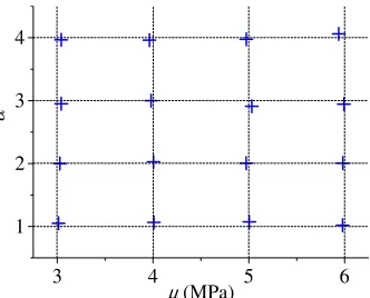
Figure 2.All identified parameters from the liner VFM on the drop-weight simulations with respect to the given parameters.
second-order central approximation. For the pre-stretching cases, a general static step was introduced before applying the dynamic loading in the explicit simulation. There were 7 different pre-deformations in order to produce engineering pre-strains of 0.1 to 0.7 with an interval of 0.1. After this pre-stretching, the same velocity boundary condition was used but applied along a plane 38 mm away from the fixed end. The one-term Ogden material model was adopted; for its parametersµandα, 1, 2, 3 and 4 were given. Thus, there were 16 simulations in total for each parameter case.
0.0 0.4 0.8 1.2 -6
-3 0 3
6 α
A
cceleration (m
m
/s
2 )
Acceleration
µ α
Time (ms)
µ(MPa)
7
10 ×
4.0 4.5 5.0 5.5
0 1 2 3 4
Figure 3.Averaged acceleration profile and the history ofµand αidentifications.
3 4 5 6
1 2 3 4
α
µ(MPa)
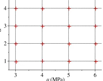
Figure 4.All identified parameters from the nonlinear VFM on the gas-gun simulations with respect to the given parameters.
3.2. Nonlinear VFM
A similar FEM was used for simulating a gas gun experiment and the nonlinear VFM procedure. The geometry was given as L =40 mm and W =11 mm. A faster velocity boundary condition was applied, which peaked at 14 m s−1with a rise time of 0.5 ms. This velocity
condition is similar to that produced in the actual gas-gun experiment. The output spacing was 10µs, i.e. an imaging speed of 100,000 fps, with a total loading duration of 1.4 ms. White Gaussian noise was added touas in the linear VFM and the calculation ofεandawas performed. These field data were then applied to Eq. (9) to identify the material parameters. Figure 3 shows the history of the parameter identifications on the simulation withµ= 4 MPa andα=2. The acceleration profile is an averaged value over the specimen surface at each time; the sign change of the acceleration indicates the moment of the wave reflection off the fixed end of the specimen. Each predicted parameter at time tk is obtained by solving Eq. (9) withε(t) anda(t) fromt =0 tot=tk. As can be seen in Fig.3, the identifications ofµandαdo not reach the given values during the incident wave period (0.0– 0.6 ms). The identifications approach the given parameters after the first wave reflection (after around 0.6 ms) in a stepwise manner. The final identified parameters are taken at the end of the time step. Using the same procedure, all other identified parameters are presented in Fig.4showing a good match with the given values.
0 10 20 30 40 50 60
0 5 10 15
Y direc
tion
(mm)
X direction (mm)
0.0 0.5 1.0
ux
(mm
)
Figure 5. Pictures of the drop-weight test before (upper) and during (bottom) loading.
4. Experiment
A sheet of a commercial EPDM rubber (Amarin Rubber & Plastic Ltd) was used for the experimental study. Three uniaxial specimens were prepared for static (L=
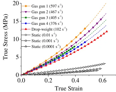
60 & W =20 mm), drop-weight and gas-gun (L =40 & W=11 mm) tests. The thickness is uniform at 2 mm. The uniaxial static test was conducted at three true strain rates: 0.01, 0.001 and 0.0001 s−1. Their true stress-strain curves
are presented in Fig.8. The strain data was measured by means of digital image correlation (DIC) software (Davis 8.2.0, LaVision) applied on test images taken by a USB camera (USB 3.0 Digital Camera, Point Grey Research, Inc.). For the DIC analysis, a white speckle pattern was made on the specimens by spray paint. The same speckle pattern was applied to the specimens for the drop-weight and gas-gun experiments. Images of the drop-weight test with this pattern is shown in Fig. 5. The drop-weight applies a displacement in thexdirection on the right hand side of the specimen. The colour map representsux field obtained from DIC analysis.
4.1. Linear VFM and drop-weight tests
In the drop-weight experiments, the EPDM specimens were located on the top of a (vertically set) long loading bar. After clamping, the effective specimen length is about 37 mm. The bar is loaded by means of a drop-weight which introduces a tensile stress wave which dynamically stretches the bottom of the specimen. A high-speed camera (FASTCAM SA5, Photron) is used to take images of the specimen at a speed of 50,000 fps. For the pre-stretching test, manual stretching was applied prior to the dynamic loading. The upper clamp was fixed and the pre-force measured with a load cell installed above. The pre-strains were calculated by comparing the distances of two pre-marked points on the specimen images.
The imaging data from one non-pre-stretching and several pre-stretching tests were analysed using DIC software to produce their displacement and strain fields. Each displacement data point was temporally fitted to a 9 degree polynomial, which was double differentiated to calculate acceleration. The test data were applied to the linear VFM procedure to obtain a series of Young’s modulus identifications. This result from the first experiment set (SET 1) is shown in Fig.6. The hatched area indicates the period where the Young’s moduli were averaged. The averaged moduli are listed in Table 1 for
0.0 0.2 0.4 0
10 20 30 40
Young
's
m
odulus (M
Pa)
Time (ms)
εx,p = 0.54 εx,p = 0.40 εx,p = 0.35 εx,p = 0.25 εx,p = 0.18 εx,p = 0.05 εx,p = 0.00
Figure 6.Identified Young’s moduli from one non-pre-stretching and six pre-stretching drop-weight tests and the application of the linear VFM.
Table 1.Averaged Young’s moduli, strain rates of the two drop-weight test sets and the identified Ogden parameters.
SET 1 SET 2
E(MPa) ε˙x(s−1) εx,p E(MPa) ε˙x(s−1) εx,p
11.8 80 0.00 12.3 103 0.00
14.9 78 0.05 12.6 96 0.08
17.1 86 0.18 13.0 108 0.14 20.6 90 0.25 14.6 102 0.15 21.0 96 0.35 17.4 122 0.23 22.2 98 0.40 20.4 118 0.31 26.6 120 0.54 23.4 109 0.34 27.7 125 0.63 Averaged ˙εx =102s−1
Optimized Ogden parameters:µ=4.39 MPa,α=1.71
identified parameter areµ=4.39 MPa andα=1.71. The strain rate value for each test in Table 1 were obtained by averaging the field data only over the deformed area. 4.2. Nonlinear VFM and gas-gun tests
The gas-gun experiment in the present study is based on the high strain rate experiment on a yarn of polymeric fibres conducted by Russell et al. [16]. For the present tests, an aluminium block (80×80×30 mm) was prepared, on which one end of two EPDM specimens was fixed. The other ends were clamped to a rigid frame attached to the barrel of the gas gun. An aluminium projectile was accelerated by the gas gun to apply impact loading on the block at speeds between 50 and 80 m s−1.
After this impact, the high-speed imaging was triggered at an imaging speed of 100,000 fps. The high-speed imaging was conducted on one of the two specimens. The captured images were analysed in the same manner as the drop-weigh test in order to produce u, ε and a. These field data were then applied to Eq. (9) to identify the Ogden parameters. There were four gas-gun tests with different impacting velocities.
Figure 7 shows the histories of the identified parameters and the averaged acceleration and strain rate profiles from one of the tests. Similarly as shown in the simulation, the identification of µ and α becomes more stable and converges in a stepwise manner as the range of the data period included in Eq. (9) increases. The stable
0.0 0.4 0.8 1.2 1.6
-6 -4 -2 0 2 4 6
Strain rate (s-1
)
α
Acceleration (m/s2
)
µ(MPa) α
Strain rate (s-1 )
Time (ms)
A
cc
ele
ratio
n
(
m
/s
2 )
µ (MPa)
×
3 6 9 12
0 2 4 6
0 200 400 600
Figure 7. Averaged acceleration & strain rate profiles and the history of theµandαidentifications of the EPDM specimens tested by the gas-gun experiment (Test 3).
0.0 0.2 0.4 0.6
0 5 10 15 20
True Stress (
M
Pa)
True Strain Gas gun 1 (597 s-1
) Gas gun 2 (467 s-1
) Gas gun 3 (405 s-1
) Gas gun 4 (376 s-1
) Drop-weight (102 s-1
) Static (0.01 s-1
) Static (0.001 s-1) Static (0.0001 s-1
)
Figure 8.Quasi-static stress strain curves and the reconstructed Ogden curves using the parameters from Tables1and2.
Table 2.Identified Ogden parameters of the EPDM specimens from the gas-gun experiment and the nonlinear VFM.
Test ε˙x(s−1) µ(MPa) α
1 597 6.52 2.12
2 467 5.70 2.05
3 405 5.26 1.95
4 376 4.87 1.85
identification period is indicated by the hatched box in Fig.7, in which theµandαvalues are averaged to obtain the final identified parameters. To calculate an average strain rate, the strain rate profile from 0.4 to 1.7 ms was chosen to be averaged, as an example. This procedure was identically repeated for all other gas-gun experiments. The identified parameters are given in Table2.
5. Discussion and conclusions
One question might arise regarding the possibility that the gas-gun and nonlinear VFM replace the drop-weight and linear VFM which need the relatively complicated pre-stretching procedures. However, it is experimentally difficult for the gas-gun experiment to produce a single loading pulse, which can generate a medium strain rate (e.g., 100 s−1), and, at the same time, a large strain with
a constant strain rate. Thus, the drop-weight experiment with the pre-stretching procedure is still useful technique to fill the gap between high and quasi-static strain rates. The drop-weight test is also advantageous for a high-speed imaging condition with a small field of view as its required deformation amplitude is small. The usefulness of the gas-gun test and its VFM procedure lies in the capability of introducing high strain rates and the experimental expedi-ency of using single loading pulse so that any unexpected material behaviour from pre-stretching can be avoided. Effort sponsored by the Air Force Office of Scientific Research, Air Force Material Command, USAF, under grant number FA8655-12-1-2015. The U.S Government is authorized to reproduce and distribute reprints for Governmental purpose notwithstanding any copyright notation thereon. The authors thank S Fuller of AFOSR and M Snyder and R Pollak of EOARD for their support. Finally we thank Professor F Pierron for his invaluable help with the Virtual Fields Method.
References
[1] Sarva S.S., Deschanel S., Boyce M.C., Chen W. (2007) Stress–strain behavior of a polyurea and a polyurethane from low to high strain rates. Polymer (Guildf) 48:2208–2213.
[2] Chen W., Zhang B., Forrestal M.J. (1999) A split Hopkinson bar technique for low-impedance materials. Exp Mech 39:81–85.
[3] Song B., Chen W. (2003) One-Dimensional Dynamic Compressive Behavior of EPDM Rubber. J Eng Mater Technol 125:294.
[4] Shergold O.A., Fleck N.A., Radford D. (2006) The uniaxial stress versus strain response of pig skin and silicone rubber at low and high strain rates. Int. J. Impact Eng. 32:1384–1402.
[5] Roland C.M., Twigg J.N., Vu Y., Mott P.H. (2007) High strain rate mechanical behavior of polyurea. Polymer (Guildf) 48:574–578.
[6] Nie X., Song B., Ge Y., et al. (2008) Dynamic Tensile Testing of Soft Materials. Exp Mech 49:451–458. [7] Pierron F., Sutton M.a., Tiwari V. (2010) Ultra High
Speed DIC and Virtual Fields Method Analysis of a Three Point Bending Impact Test on an Aluminium Bar. Exp Mech 51:537–563.
[8] Moulart R., Pierron F., Hallett S., Wisnom M. (2011) Full-Field Strain Measurement and Identification of Composites Moduli at High Strain Rate with the Virtual Fields Method. Exp Mech 51:509–536. [9] Pierron F., Forquin P. (2012) Ultra-High-Speed
Full-Field Deformation Measurements on Concrete Spalling Specimens and Stiffness Identification with the Virtual Fields Method. Strain 48:388–405. [10] Pierron F., Zhu H., Siviour C. (2014) Beyond
Hopkinson’s bar. Philos Trans R Soc A Math Phys Eng Sci 372:20130195.
[11] Pierron F., Gr´ediac M. (2012) The virtual fields method?: extracting constitutive mechanical para-meters from full-field deformation measurements (Springer, New York)
[12] Ogden R.W. (1972) Large Deformation Isotropic Elasticity – On the Correlation of Theory and Experiment for Incompressible Rubberlike Solids. Proc R Soc London A Math Phys Sci 326:565–584. [13] ABAQUS (2011) ABAQUS 6.11 analysis user’s
manual. Abaqus 6.11 Doc.
[14] Promma N., Raka B., Gr´ediac M., et al. (2009) Ap-plication of the virtual fields method to mechanical characterization of elastomeric materials. Int J Solids Struct 46:698–715.
[15] Palmieri G., Sasso M., Chiappini G., Amodio D. (2011) Virtual Fields Method on Planar Tension Tests for Hyperelastic Materials Characterisation. Strain 47:196–209.