Article
High-throughput of measure-preserving integrators
for constant temperature molecular dynamics
simulations on GPUs
Luis Guarneros-Nolasco 1,5, Ketzasmin A. Terrón-Mejía 5, Jorge Mulia-Rodríguez 3, Daniel Osorio-González 4, Roberto López-Rendón 1, Felipe Rodríguez-Romero 5,*
1 Laboratorio de Bioingeniería Molecular a Multiescala, Facultad de Ciencias, Universidad Autónoma del
Estado de México, Av. Instituto Literario 100, Toluca 50000, Mexico; [email protected] (L.G.-N.); [email protected] (R.L.-R.)
2 Laboratorio de Venómica Computacional, Facultad de Ciencias, Universidad Autónoma del Estado de
México, Av. Instituto Literario 100, Toluca 50000, Mexico; [email protected] (F.R.-R)
3 Laboratorio de Biotermodinámica Computacional, Facultad de Ciencias, Universidad Autónoma del
Estado de México, Av. Instituto Literario 100, Toluca 50000, Mexico; [email protected] (J.M.-R)
4 Laboratorio de Biofísica Molecular, Facultad de Ciencias, Universidad Autónoma del Estado de México,
Av. Instituto Literario 100, Toluca 50000, Mexico; [email protected] (D.O.-G)
5 Instituto Tecnológico Superior de Zongolica, Km. 4 Carretera a la Compañía, Zongolica, Veracruz 95005,
Mexico; [email protected] (L.G.-N.); [email protected] (K.A.T.-M.) * Correspondence: [email protected]; Tel.: +52 722 296 5556
Abstract: Molecular dynamics simulation is currently the theoretical technique eligible to simulate a wide range of systems from soft condensed matter to biological systems. However, of the excellent results that the technique has arrogated, this approach remains computationally expensive, but with the emergence of the new supercomputing technologies bases on graphics processing units graphical processing units-based systems GPUs, the perspective has changed. The GPUs allow performing large and complex simulations at a significantly reduced time. In this work, we present recent innovations in the acceleration of molecular dynamics in GPUs to simulate non-Hamiltonian systems. In particular, we show the performance of measure-preserving geometric integrator in the canonical ensemble, that is, at constant temperature. We provide a validation and performance evaluation of the code by calculating the thermodynamic properties of a Lennard-Jones fluid. Our results are in excellent agreement with reported data reported from literature, which were calculated with CPUs. The scope and limitations for performing simulations of high-throughput MD under rigorous statistical thermodynamics in the canonical ensemble are discussed and analyzed.
Keywords: High-Throughput Molecular Dynamics (HTMD) simulations; Nosé-Hoover Chain (NHC); Canonical ensemble; Graphics Processing Units (GPUs).
1. Introduction
The accelerated use of molecular simulation methods, such as molecular dynamics (MD) simulations, has motivated an increasing interest in the implementation of rigorous algorithms in modern supercomputing technologies, which is a difficult task. Due to the purely numerical nature of MD method, which emerge from the laws of statistical mechanics, they require the use of efficient schemes to sample the phase space, maintaining control of thermodynamic variables at large scales of time and length. The combination of powerful computational technologies and the strict laws of statistical mechanics placed in a same simulation code is a great challenge nowadays.
From a conceptual perspective, MD simulations (based on the integration of Newton’s equations motion) are considered as numerical experiments that provides the means to sample the thermodynamic space of a given system through its evolution dynamical. In MD simulations, these
spaces or thermodynamic ensembles are characterized according to the type of physical variables that are to be evaluated. For example, the simplest case is where it is required to keep the energy constant, this case is the so-called microcanonical ensemble (NVE), where the thermodynamic condition is to maintain the energy constant (E), as well as the volume (V) and number of particles (N). However, for comparations with experimental conditions, it is often convenient perform simulations at constant temperature, which leads us to have a system in the canonical ensemble (NVT). In this case, the thermodynamic condition is to maintain the temperature constant (T), as well as the volume (V) and number of particles (N). The NVT ensemble is somewhat more difficult to generate than the NVE ensembles due to the requirement that the kinetic energy fluctuations must generate the correct distribution function corresponding to the ensemble. Temperature control algorithms comprise one of the fundamental parts in MD simulations.
Generally, when the Newtonian MD scheme it is modified to maintain the temperature constant is through of the tools called a thermostat algorithms (TAs). An efficient thermostat must meet certain requirements required of the statistical mechanics. For example, give a canonical distribution of speeds, and be ergodic, etc. Not only averages, but also fluctuations (dispersions) away from the average are also important. Several strategies to improve simulations at the canonical ensemble have been suggested in the literature [1-5]. The simplest method is through the periodic scaling of velocities; this method is economically and numerically stable. However, it does not guarantee that a canonical space distribution is obtained, but they are still commonly used. The lack of ergodicity for some thermostat algorithms or for different temperature ranges can lead to a dynamic that does not correctly reproduce the expected thermodynamic properties [6-9].
Simulating a thermal bath is not a simple task. To achieve an accurate and efficient integration in the constant-temperature ensemble, additional variables may be added to create a “thermostat” that controls the temperature of the simulated system [10]. From this idea arise the so-called extended Hamiltonian methods or Non-Hamiltonian methods [11-14]. These variables or extended degrees of freedom regulate the time-averaged values of temperature in order to reproduce as accurately as possible the phase space in the considered ensemble. However, the use of this type of methods, although are accurate, are should be used with care, for example, the mass of extended variables must be carefully chosen as they affect spontaneous fluctuations in the system. Lippert et. al exposed computational challenges that involve controlling the temperature of a system using external degrees of freedom [15]. Two fundamental observations were made. One of them was the high computational cost that carries the instantaneous updates of extended degrees of freedom. Second, observation to the wide separation between the timescales associated with the extended degrees of freedom and those associated with particle motion. The extended degrees of freedom generally evolve on timescales much longer than those of particle motion; this can result in numerical inaccuracy if the numerical precision employed is insufficient.
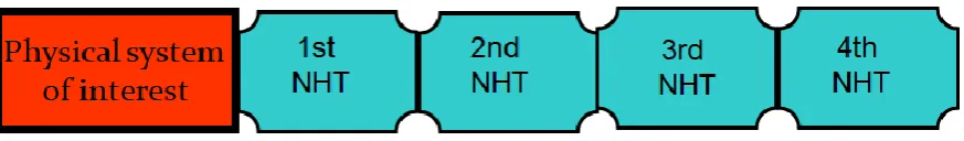
Figure 1. Schematic representation of the NHC method and its operating. The temperature of the physical system (red box) is controlled by the mechanism of the NHC equations (all four green boxes). That is, the first Nosé-Hoover thermostat (1st NHT) in the chain is coupled to the physical system, the second (2nd NHT) is coupled to the first Nosé-Hoover, the third (3rd NHT) is coupled to the second thermostat, the (4th NHT) is coupled to the third thermostat Nosé-Hoover, and so on, until forming a collective system of Nosé-Hoover chains (NHC).
When using non-Hamiltonian equations of motion, such as NHC equations, the numerical integrator should be consistent with a non-Hamiltonian generalization of Liouville’s theorem [22, 23]. That mean that the integrator must be symplectic, that is, must conserve exactly the invariant phase-space volume, must have an approximate energy conservation, and time reversibility between other properties [24]. A numerical integrator that achieves this is known as a “ measure-preserving” algorithm. These numerical algorithms are based on decompositions of exponential operators, and the error in the total energy of the system is bounded [25]. Also, these algorithms represent the explicit integration of non-Hamiltonian dynamical systems. So far, Tuckerman et al. [26] have developed a consistent classical statistical theory of certain non-Hamiltonian dynamical systems and have developed a “systematic way” of designing equations of motion of extended molecular dynamics which are known as MTK equations, from Martyna, Tobias and Klein authors.
MTK algorithms are already applicable to a wide range of scientific problems and have been expanding their applications in several areas, such as: Physical Chemistry [27], Theoretical and Computational Chemistry [28], Materials Engineering [29], Macromolecular and Materials Chemistry [30], Biochemistry [31], Cellular and Cell Biology science [32], and so on. The implementation of the MTK algorithms is not trivial and its evaluation is computationally expensive. So far, major MD codes such as LAMMPS [33], AMBER [34], HOOMD-blue [35] and GROMACS [36] have implemented the MTK algorithms, being LAMMPS the most used code with these algorithms. But nevertheless, these codes were designed and work in programming environments in CPUs. On the other hand, with the advent of graphics processing units (GPUs), the field of High-throughput MD (HTMD) has become a fundamental tool for pharmaceutical research [37], accelerate the innovation in materials research [38], in revolutionizing the genome-wide [39], to explore large effects of structural changes ensemble of proteins [40], for drug discovery [41], just to mention a few applications. However, these areas have been developed using huge and expensive CPUS clusters. Unfortunately, the generation of HTMD codes designed exclusively for perform molecular simulations on GPUs is very scarce. ACEMD [42] is the only code of MD specially optimized to run on GPUs and it is one of the world’s fastest molecular dynamics engines. Nevertheless, ACEMD works with Langevin type thermostats, and to date, has not yet implemented the MTK algorithms.
reported today are of this number of atoms, but with a production of ns/day of half or less than half. So far, no code with those capabilities has been reported using NHC thermostat.
2. Methodology
It is well-known that a symplectic integrator conserves the Hamiltonian and therefore achieves stable integration over a long time. This is because there exists a value that is exactly conserved by the approximated propagator. These numerical methods are based on the decompositions of exponential operators. A system that preserve the generalized phase-space metric, it will be consistent with the generalization of Liouville’s theorem. The details of Liouville operator algorithms derivation for non-Hamiltonian systems, such as NHC thermostat, can be found in original papers sources [43-46], therefore we shall only outline the main NHC equations.
In order to generate a sampling of the canonical distribution (NVT), Hamilton’s equations must be supplemented by a mechanism that allows the system to exchange energy with its surroundings. One popular method for mimicking the influence of the surroundings in MD is so called extended phase space approach. As already mentioned in the Introduction section, Nosé-Hoover method is one of the best schemes to generate a canonical distribution but has ergodicity problems. The failure of this approach was solved by Martyna et al. introducing the NCH thermostat [21]. The main idea behind the NCH thermostat is that the physical position and momentum variables of the particles in the system are coupled to additional phase space variables that mimic the effect of the surroundings by controlling the fluctuations in the instantaneous kinetic energy.
The NHC thermostat [21] is a non-Hamiltonian MD scheme for generating the canonical ensemble. In this method, the ordinary phase space is extended to include a set of M thermostat variables 𝜂1, … 𝜂𝑀 and their conjugate momenta 𝑝𝜂1, … 𝑝𝜂𝑀, which serve to drive the fluctuations of the kinetic energy in such a way that they average to the proper canonical value. These variables act as a heat bath coupled to the system. The equations of motion for an NHC system are
𝐫 𝑖̇ = 𝐩𝑖 𝑚𝑖 𝐩̇𝑖= 𝐅𝑖− 𝑝𝜂𝑖 𝐐1 𝐩𝑖 𝜂̇𝑘= 𝑝𝜂𝑘 𝑄𝑘
𝑘 = 1, … , 𝑀
𝑝𝜂𝑘= 𝐺𝑘− 𝑝𝜂𝑘+1 𝑄𝑘+1
𝑝𝜂𝑘 𝑘 = 1, … , 𝑀 − 1
𝑝̇𝜂𝑀= 𝐺𝑀 (1) where the thermostat forces are
𝐺1= ∑ 𝐩𝑖2 𝑚𝑖 𝑁
𝑖=1
− 3𝑁𝑘𝑏𝑇
𝐺𝑘= 𝑝𝜂𝑘−12
𝑄𝑘−1 − 𝑘𝑏𝑇 (2)
The parameter 𝑄1, … 𝑄𝑀 are mass-like parameters (having units of energy*time2) that determine the time scale on which the heat-bath variables evolve, and 𝑘𝑏 is the Boltzmann constant. The term −(𝑝𝜂1/𝑄1)𝐏𝑖 in the momentum equation acts as a kind of dynamic frictional force. Although the average 〈𝑝𝜂1〉 = 0, instantaneously, 𝑃𝜂1 can be positive or negative and can, therefore, act to damp or boost the momentum. According to the equation for 𝑃𝜂1, if the kinetic energy is larger than 3𝑁𝑘𝑏𝑇/2, 𝑃𝜂1, it will increase and have a greater damping effect on the momenta, while if the kinetic energy is less than 3𝑁𝑘𝑏𝑇/2, 𝑃𝜂1 will decrease, become negative, and have a boosting effect. In this way, the NHC system acts as a “thermostat” regulating the kinetic energy. In a similar manner, the (𝑘 + 1)th heat-bath variable serves to modulate the fluctuations of the kth variable so that each heat-bath variable (except the Mth variable) is “driven” to have a proper canonical average. Equations (1) have the conserved energy
𝐻′= 𝐻(𝐩, 𝐫) + ∑𝑝𝜂𝑘 2
2𝑄𝑘 𝑀
𝑘=1
+ 𝑘𝑏𝑇 [𝑑𝑁𝜂1+ ∑ 𝜂𝑘 𝑀
𝑘=2
where 𝐻(𝐩, 𝐫) is the Hamiltonian of the physical system. When 𝑀 = 1, the NHC system reduces to the simpler Nosé-Hoover system [19], which does not generate the corresponding canonical distribution.
3. Results
3.1. Code validation
In this section, we show the results of an implementation of NHC thermostat on GPUs. First, we performed the validation of the code simulating a system composed of 864 particles of a Lennar-Jones (LJ) fluid. A comparison with the data of the literature is included, we show that the equilibrium properties are the same for the simulation time considered here, but our data are calculated in GPUs while those of literature are calculated in CPUs. The details of the simulations presented can be found in appendix A of this manuscript.
The Figure 2 shows the equilibrium properties of LJ fluid in bulk phase. The comparison between literature data (calculations in CPUs) from Johnson et al. [47] and simulation data from this work (calculations in GPUs) is presented. Figure 2a shows the behavior of the potential energy as a function (U∗) of density (𝜌∗) for a wide range of temperatures, from T = 2.0 to T = 6.0. These values are in reduced units. In our case, the error bars are included. Figure 2b shows the behavior of the pressure (P∗) as a function of density (𝜌∗) for a wide range of temperatures, from T = 2.0 to T = 6.0. All values are in reduced units. We can see that the agreement between the data of the literature calculated in CPUs and the data calculated in this work in GPUs is excellent. This is a test of the excellent implementation of the NHC algorithm in GPUs. These results show that the canonical ensemble given by the NHC algorithm correctly produces thermodynamic properties in equilibrium, performed in GPUs as is showed in this work.
Figure 2. Equilibrium properties of Lennard-Jones fluid in bulk phase: (a) Potential energy vs. density. The blue line corresponds to literature data from Johnson et al. [47]., which were calculated in CPUS, while the red dotted line are simulation data from this work but calculated in GPUs. The symbol of the error bars is included in our calculations; (b) Pressure vs. density. The continuous lines correspond to the data reported by Johnson et al. [47], while the data with symbols correspond to data obtained in this work. All units are dimensionless.
For a thermostat to be entirely consistent with the canonical ensemble, it should generate total energies according to the Boltzmann distribution for that system and generate kinetic energies consistent with the Maxwell−Boltzmann distribution [23]. To verify this rule, first we evaluate the evolution of the conserved quantity (𝛥𝑈) given by equation (3) for a LJ fluid at T∗= 2.0, 𝜌∗= 0.7, and 𝑁 = 864. The result is displayed in Fig. 3A. The instantaneous (𝛥𝑈) has the definition |(𝑈𝑖− 𝑈0)/𝑈0| and the cumulative average (𝛥𝑈) is denoted by 𝛥𝑈 =
1
Figure 3. (a) Evolution of conserved quantity (𝛥𝑈) as a function of simulation time (ps). The red line corresponds to average energy while the black line corresponds to instant energy; (b) Histogram of cumulative momentum distribution obtained from a trajectory calculated using NHC method. For this case T∗= 2.0, 𝜌∗= 0.7, and 𝑁 = 864.
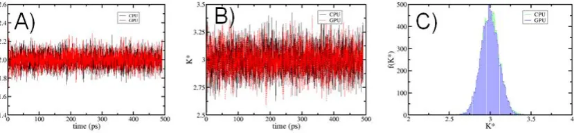
The NHC motion equations increase the calculation time and the complexity due to the coupling of the thermostats; this causes the ergodicity of the dynamics to increase when increasing the available phase space of the dynamics. One of the main goals of using GPUs in MD simulations is to break with the time/length scales, that is, to simulate larger systems and longer times, preserving the correct application of the laws of statistical mechanics. To show the effectiveness of the NHC algorithm in the canonical assembly, we analyze the evolution of the temperature reduce ( T∗), the kinetic energy reduced ( K∗), as well as the distribution of the kinetic energy reduce 𝑓( K∗). The results are show in the figure 4. We can see that 𝑓( K∗) obeys to the correct distribution dictated by the canonical assembly [25]. This result shows a good agreement with similar results in the evaluation of geometrical properties that are applied to the algorithms designed to maintain the temperature in the canonical ensemble [3]. It is important to emphasize the conservation of temperature, which shows any no drift. The calculations on CPUS presented in this section were performed with an in-house code.
Figure 4. Sampling of temperature between CPUS and GPUs platforms; (a) Evolution of the reduced temperature ( T∗) of the system at equilibrium; (b) The behavior of the reduced kinetic energy ( K∗); (c) The numerical distribution reduced kinetic energy 𝑓( K∗) for the same system is showed. The details of these simulations can be found in the Appendix A. All thermodynamics are reported in dimensionless units.
3.2. Code performance
latest GPUs technologies. As we mentioned before, the true power of using GPUs is to simulate systems composed of a large number of atoms, as clusters based on GPUs technologies allow.
To know some advantages like high efficiency, high speed and low cost of the NHC thermostat on GPUs, the execution time per step of MD and the speedup were measure, both parameters as a function of the number of particles. The result is shown in figure 5. We observe from Figure 5A, that the computational cost of time per step increases exponentially in the CPUs. As the number of particles increases, the time per step also increases. In the GPUs, the computational cost of time per step is practically constant. Speedup in Figure 5B is measured as the ratio of wall time elapsed for carrying out a specific simulation. In this case, we observe that for a system of 4000 particles a speedup of 45is achieved, while a system of 23328achieves a speedup of 60, therefore, the speedup achieved by going from a system of 4000 particles to a system of 23328 is of the order of 25. A speedup of this magnitude is significant because of the wide applications of MD simulations to biological systems. These tests were measured in the GPU model GTX-1080 for systems of LJ particles.
Figure 5. Performance of NHC thermostat on GPUS: (a) Performance CPU vs. GPU of time per step as a function of particles number; (b) Speedup of NHC thermostat as a function of particles number. These tests were measured in the GPUs model GTX-1080 for a system of 4000, 6912, 10976, 16384 and 23328 particles. The Speedup obtained by migrate the NHC algorithms to GPUs is approach 60 times faster than the CPU version.
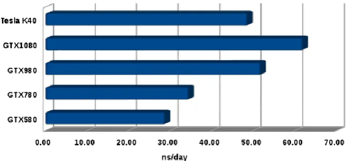
Figure 6. Performance Evaluation and Benchmarking of NHC thermostat in different GPUs architectures. The performance of our code is tested on a system of constituted by 10976 Lennard-Jones type particles.
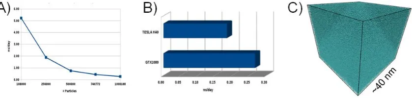
Currently, our code can simulate up to 1.2 million particles. The benchmarking production is presented in the Figure 7. Simulating more than one million particles is a challenge that keeps many research groups busy. This size of systems is the maximum that a GPUs supports, due to the capacity of the memory. GPUs with greater memory capacity could simulate larger systems, and of course with a higher ns/day production. Figure 7A shows the decay of ns / day production as the particle number increases. This behavior is normal due to the cost of calculating the forces. The maximum size that we manage to simulate is about of one 1.2 million of LJ particles, obtaining only 0.27 ns/day on GPUs model GTX-1080, so it is seen more clearly in figure 7B. Figure 7C shows an example of the configuration of this system, which measures approximately 40 nm. That order of magnitude is of great importance where the capabilities of the HTMD are exploited.
Figure 7. HTMD of NHC thermostat performance on GPUs; (a) Maximum performance on a GPUs GTX-1080; (b) Comparations of production in ns/day between two GPUs architectures to simulate one million of LJ particles; (c) A snapshot of a system composed by one million of particles.
4. Discussion
The key contribution of HTMD molecular simulations technologies is to accelerate the innovation in research both simple systems and complex systems. We think that new computational algorithms and strong collaborations between chemists, physicists, biologists, mathematicians, engineers and medical professionals will reinforce this area of research. However, the problems and challenges related to biomolecules, which are often expensive in the sense of numerical simulation, open a research window with a major difficult to answer. A question that has not been fully addressed to date is to what extent the kinetic properties can be reproduced correctly, this using MD to see extent simulations can be accelerated by these simulations methods [49].
to run simulations locally for longer periods of time and with greater flexibility. Finally, we see that the race to have more and better MD codes in GPUS is in constant growth, and we need more innovation in this sense.
5. Conclusions
The evolution and innovation in the development MD software on GPUs is in constant expansion. However, the use of GPUs acceleration of condensed-phase matter MD simulations is still in its infancy. The pressure to achieve maximum performance has led to the use of approximations in statistical methodologies trying to avoid a real rigorous validation. The development of MD codes in GPUs seems to be an established and extremely active field, however, very few codes can be considered ready for production and even very few achieve the desired goal of making direct comparisons with real experiments, without making approximations. However, the current benefits of GPUs are enticing, and this is driving both code and hardware development. Despite the substantial progress made in the development of the code, the difficulty in programming GPUs devices persists, programming complex algorithms such as the NHC thermostat makes some groups choose to implement simpler thermostats, which are efficient at long times, as example explicit are the NH and Langevin thermostats. With constant anticipated release of new technology NVIDIA will undoubtedly bring more competition in the development of more efficient software with more demanding implementations such as those presented in this work. It is anticipated that with the release of new versions of GPUs, MD codes will evolve rapidly, while research with these methodologies will increase exponentially in the coming years, but the limitation of implementing complex methodologies such as those presented in this paper is a latent challenge.
Author Contributions: L. G.-N. and F. R.-R. Software, Supervision and writing—original draft; J. M.-R. Methodology; D. O.-G. Methodology; R.L.-R., K.A.T.-M. and F.R.-R. Conceptualization,. R.L.-R. and F.R.-R Funding acquisition, Project administration, Resources. All authors contributed to the reading, writing, and approval of the original manuscript.
Funding: F.R.R. and R.L.R. thank the financial support from SIyEA-UAEM (Projects 3475/2013CHT and 3585/ 2013CHT).
Acknowledgments: All simulations reported in this work and the development of our HTMD code were performed at the Supercomputer OLINKA, located at the Laboratory of Molecular Bioengineering at Multiscale (LMBM), at the Universidad Autónoma del Estado de México. L.G.-N. acknowledges CONACyT México for supporting his PhD studies.
Conflicts of Interest: The authors declare no conflict of interest. The funders had no role in the design of the study; in the collection, analyses, or interpretation of data; in the writing of the manuscript, or in the decision to publish the results.
Code available: The code presented in this paper is available online from our web site: http://www.himd.uaemex-labs.org.mx/
Appendix A
Computational details. The performed simulations in this work are split in two main blocks. The first one corresponds to the validation of the code developed, and the second one regards the scope of performance obtained at the implementation of Nose-Hoover chains in GPU architecture. For the validation of the code, we reproduced some data reported by Jonson et. al. [47]. These data correspond to a fluid of Lennard-Jones particles, simulated in a canonical ensemble (NVT), the conditions of temperature and density are in range of 2.0 to 6.0 and 0.1 to 1.3 respectively. These intervals of thermodynamic conditions exclude metastable points over solidification and vaporization curves [47], while the number of particles in the system is 864. Other parameters of simulation are time step ∆𝑡 = 0.002, characteristic time scale of particles 𝜏𝑇 = 0.2, cutoff radius 𝑟𝐶 = 4.0𝜎, Verlet radius 𝑟𝑉= 4.5𝜎. Units of reference selected are: size of particles 𝜎 = 3.405Å, mass of particles 𝑚 = 39.95𝑔𝑚𝑜𝑙−1 and the depth of potential 𝜀/𝑘
algorithm of integration [50] and the Nose-Hoover chains as thermostat for keeping the temperature in the ensemble NVT.
Second block of simulations is focused on analyzing the performance of NHC executed in the GPU. For these simulations, it is used one system of LJ particles under the same thermodynamic parameters (𝜌 = 0.7,𝑇 = 2.0), but in this case the number of particles is 4000, 6912, 10976, 16384 and 23328. Next group of simulations is centered on exploring the behavior of the code in different models of the GPUs, the selected system for this test is of 10976 particles under the thermodynamics conditions. The models of GPUs used are GTX580, GTX780, GTX980, GTX1080 and Tesla K40. Finally, the last group of simulations explores the capacity with respect to the size of the systems that will be studied with this code developed. We estimated real time simulated that will reach systems with 108000, 256000, 500000, 740772 and 1000118 particles in the canonical ensemble, using the thermostat of Nose-Hoover chains. All the quantities are presented in reduced units unless otherwise indicated.
References
1. Hu, Y.; Sinnott, S.B. Constant temperature molecular dynamics simulations of energetic particle–solid collisions: comparison of temperature control methods. Journal of Computational Physics, 2004, 200, 251–266, doi:10.1016/j.jcp.2004.03.019.
2. Houndonougbo, Y. A.; Laird, B. B. Constant-temperature molecular-dynamics algorithms for mixed hard-core/continuous potentials J. Chem. Phys. 2002, 117, 1001-1009, http://dx.doi.org/10.1063/1.1485072
3. Tapias, D.; Sanders, D.P.; Bravetti, A. Geometric integrator for simulations in the canonical ensemble. J. Chem. Phys. 2016, 145, 084113, http://dx.doi.org/10.1063/1.4961506.
4. Samoletov, A.A.; Dettmann, C. P.; Chaplain, M.A.J. Thermostats for “Slow” Configurational Modes. J. Stat. Phys. 2007, 128, 1321–1336. DOI: 10.1007/s10955-007-9365-2.
5. Hoover, W.G.; Sprott, J.C.; Patra, P.K. Ergodic time-reversible chaos for Gibbs’ canonical oscillator. Physics Letters A 2015, 379, 2935–2940. http://dx.doi.org/10.1016/j.physleta.2015.08.034
6. Hoover, W.G.; Sprott, J.C.; Hoover, C.G. Ergodicity of a singly-thermostated harmonic oscillator. Commun Nonlinear Sci Numer Simulat 2016, 32, 234–240. http://dx.doi.org/10.1016/j.cnsns.2015.08.020
7. Jepps, O.G.; Rondoni, L. Deterministic thermostats, theories of nonequilibrium systems and parallels with the ergodic condition. J. Phys. A: Math. Theor. 2010, 43, 133001. doi:10.1088/1751-8113/43/13/133001.
8. Legoll, F.; Luskin, M.; Moeckel, R. Non-Ergodicity of the Nosé–Hoover Thermostatted Harmonic Oscillator. Arch. Rational Mech. Anal.2007, 184, 449–463, DOI: 10.1007/s00205-006-0029-1.
9. Legoll, D.; Luskin, M.; Moeckel, R. Non-ergodicity of Nosé–Hoover dynamics Nonlinearity 2009, 22, 1673–
1694, doi:10.1088/0951-7715/22/7/011
10. G. J. Martyna, M. E. Tuckerman, D. J. Tobias, and M. L. Klein, Explicit reversible integrators for extended systems dynamics Mol. Phys. 1996, 87, 1117-1157, https://doi.org/10.1080/00268979600100761
11. Ezra, G.S. Reversible measure-preserving integrators for non-Hamiltonian systems J. Chem. Phys. 2006, 125, 034104, DOI: 10.1063/1.2215608
12. Sergi, A.; Ferrario, M. Non-Hamiltonian equations of motion with a conserved energy Physical Review E, 2001, 64, 056125, https://doi.org/10.1103/PhysRevE.64.056125
13. Ciccotti, G.; Ferrario, M. Holonomic Constraints: A Case for Statistical Mechanics of Non-Hamiltonian Systems Computation 2018, 6, 11; doi:10.3390/computation6010011
14. Giusteri, G.G.; Podio-Guidugli, P.; Fried, E. Continuum balances from extended Hamiltonian dynamics J. Chem. Phys., 2017, 146, 224102, http://dx.doi.org/10.1063/1.4984823
15. Lippert, R. A.; Predescu, C.; Ierardi, D.J.; Mackenzie, K.M.; Eastwood, M.P.; Dror, R.O.; Shaw, D. E.
Accurate and efficient integration for molecular dyna11mics simulations at constant temperature and pressure J. Chem. Phys. 2013, 139, 164106, http://dx.doi.org/10.1063/1.4825247
16. Berendsen, H.J.C.; Postma, J.P.M; van-Gunsteren, W.F.; DiNola, A.; Haak, J.R. Molecular dynamics with coupling to an external bath. J. Chem. Phys.1984, 81, 3684-3690, https://doi.org/10.1063/1.448118.
17. Andersen, H.C. Molecular dynamics simulations at constant pressure and/or temperature. J. Chem. Phys. 1980, 72, 2384-2393. https://doi.org/10.1063/1.439486.
18. Nosé, S. A unified formulation of the constant temperature molecular dynamics methods.J. Chem. Phys.
19. Hoover, W.G. Canonical dynamics: Equilibrium phase-space distributions. Phys. Rev. A1985, 31, 1695-1697.
https://doi.org/10.1103/PhysRevA.31.1695.
20. Martyna, G.J.; Tuckerman, M.E. Symplectic reversible integrators: Predictor–corrector methods J. Chem. Phys. 1995, 102, 8071-8077, https://doi.org/10.1063/1.469006
21. Martyna, G.J.; Klein, M.L.; Tuckerman, M. Nosé–Hoover chains: The canonical ensemble via continuous dynamics, J. Chem. Phys. 1992, 97, 2635-2643. https://doi.org/10.1063/1.463940
22. Tuckerman, M.E.; Mundy, C.J.; Martyna, G.J. On the classical statistical mechanics of non-Hamiltonian systems.Europhys. Lett. 1999, 45, 149-155, https://doi.org/10.1209/epl/i1999-00139-0
23. Tuckerman, M.E.; Liu, Y.; Ciccotti, G.; Martyna, G.J. Non-Hamiltonian molecular dynamics: Generalizing Hamiltonian phase space principles to non-Hamiltonian systems J. Chem. Phys. 2001, 115, 1678-1702,
https://doi.org/10.1063/1.1378321
24. McLachlan, R.I.; Quispel, R.R.W. Geometric integrators for ODEs, J. Phys. A: Math. Gen. 2006, 39, 5251–5285 doi:10.1088/0305-4470/39/19/S01
25. Tuckerman, M.E.; Martyna, G.J. Understanding Modern Molecular Dynamics: Techniques and
Applications, J. Phys. Chem. B 2000, 104, 159-178, DOI: 10.1021/jp992433y
26. Tuckerman, M.E. Statistical Mechanics: Theory and Molecular Simulation, Oxford University Press, 1st Edition, 2013; 696 pages, ISBN-13: 978-0198525264.
27. Andoh, Y.; Yoshii, N.; Yamada, A.; Okazaki, S. Evaluation of atomic pressure in the multiple time‐step integration algorithm 2017, 38, 704-713, DOI: 10.1002/jcc.24731.
28. Van Houteghem, M.; Ghysels, A.; Verstraelen, T.; Poelmans, W.; Waroquier, M.; Van Speybroeck, V. Critical Analysis of the Accuracy of Models Predicting or Extracting Liquid Structure Information J. Phys. Chem. B, 2014, 118, 2451–2470, DOI: 10.1021/jp411737s
29. Sencer Selcuk, S.; Xunhua Zhao, X.; Selloni, A.; Structural evolution of titanium dioxide during reduction in high-pressure hydrogen Nature Materials 2018, 17, 923–928, https://doi.org/10.1038/s41563-018-0135-0 30. Allen, D.; Lorenz, C.D. A novel method for constructing continuous intrinsic surfaces of nanoparticles J.
Mol. Model. 2017, 23, 219, DOI 10.1007/s00894-017-3378-9
31. Ayee, M.A.A.; LeMaster, E.; Shentu, T.P.; Singh, D.K.; Barbera, N.; Soni, D.; Tiruppathi, Ch.; Subbaiah, P.V.; Berdyshev, E.; Bronova, I.; Cho, M.; Akpa, B.S.; Levitan, I. Molecular-Scale Biophysical Modulation of an Endothelial Membrane by Oxidized Phospholipids Biophysical Journal, 2017, 112, 325–338, https://doi.org/10.1016/j.bpj.2016.12.002
32. Sadeghi, M.; Weik, T.R.; Noé, F. Particle-based membrane model for mesoscopic simulation of cellular dynamics J. Chem. Phys. 2018, 148, 044901, https://doi.org/10.1063/1.5009107
33. S. Plimpton, Fast Parallel Algorithms for Short-Range Molecular Dynamics, J Comp Phys, 117, 1-19 (1995).
34. Cheng, A.; Merz., K.M. Application of the Nose´-Hoover Chain Algorithm to the Study of Protein Dynamics J. Phys. Chem. 1996, 100, 1927-1937, DOI: 10.1021/jp951968y
35. J. A. Anderson, C. D. Lorenz, and A. Travesset. General purpose molecular dynamics simulations fully implemented on graphics processing units Journal of Computational Physics 227(10): 5342-5359, May 2008. 10.1016/j.jcp.2008.01.047
36. Hess B, Kutzner C, van der Spoel D, Lindahl E. GROMACS 4: Algorithms for highly efficient, load balanced, and scalable molecular simulation. J. Chem. Theory. Comput. 2008, 4, 435-447.
37. Stanley, N.; De Fabritiis, G. High throughput molecular dynamics for drug discovery In Silico Pharmacology 2015, 3, 3 DOI 10.1186/s40203-015-0007-0.
38. Erucar, I.; Keskin, S. High-Throughput Molecular Simulations of Metal Organic Frameworks for CO2 Separation: Opportunities and Challenges Front. Mater.2018, 5, 4, doi: 10.3389/fmats.2018.00004
39. Hospital, A.; and Josep Ll Gelpi, J.LI. High-throughput molecular dynamics simulations: toward a dynamic view of macromolecular structure WIREs Comput Mol Sci2013, doi: 10.1002/wcms.1142
40. Yamamoto, E.; Kalli, A.C.; Yasuoka, K.; Sansom, M.S.P. Interactions of Pleckstrin Homology Domains with Membranes: Adding Back the Bilayer via High-Throughput Molecular Dynamics Structure2016, 24, 1421–
1431, http://dx.doi.org/10.1016/j.str.2016.06.002
41. Harvey, M.J.; De Fabritiis, G. High-throughput molecular dynamics: the powerful new tool for drug discovery Drug Discovery Today2012, 17, 1059-1062, http://dx.doi.org/10.1016/j.drudis.2012.03.017
43. M.E.; Alejandre, J.; López-Rendón, R.; Jochim, A.L.; Martyna, G.J. A Liouville-operator derived measure-preserving integrator for molecular dynamics simulations in the isothermal–isobaric ensemble. J. Phys. A: Math. Gen. 2006, 39, 5629–5651, doi:10.1088/0305-4470/39/19/S18.
44. Yu, T.-Q.; Alejandre, J.; López-Rendón, R.; Martyna, G.J.; Tuckerman, M.E. Measure-preserving integrators for molecular dynamics in the isothermal–isobaric ensemble derived from the Liouville operator. Chem. Phys. 2010, 370, 294–305, doi: 10.1016/j.chemphys.2010.02.014.
45. Yu, T.-Q.; Tuckerman, M.E. Constrained molecular dynamics in the isothermal-isobaric ensemble and its adaptation for adiabatic free energy dynamics Eur. Phys. J. Special Topics 2011, 200, 183–209, DOI: 10.1140/epjst/e2011-01524-x
46. Romero-Bastida, M.; López-Rendón, R. Anisotropic pressure molecular dynamics for atomic fluid systems.
J. Phys. A: Math. Theor. 2007, 40, 8585–8598, doi:10.1088/1751-8113/40/29/026.
47. Johnson, J.K.; Zollweg, J.A.; Gubbins K.E. The Lennard-Jones equation of state revisited Mol. Phys. 1993, 78, 591-618, https://doi.org/10.1080/00268979300100411
48. Olinka Supercomputer. Available online: http://www.olinka.uaemex-labs.org.mx/.
49. Feig, M. Kinetics from Implicit Solvent Simulations of Biomolecules as a Function of Viscosity J. Chem. Theory Comput. 2007, 3, 1734-1748, DOI: 10.1021/ct7000705.