Measuring Strategic Communications

(1)

University of South Carolina

Scholar Commons

Theses and Dissertations

2016

Mathematical Modeling Of Transport And

Corrosion Phenomenon Inside High Temperature

Molten Salt Systems

Bahareh Alsadat Tavakoli Mehrabadi University of South Carolina

Follow this and additional works at:https://scholarcommons.sc.edu/etd Part of theChemical Engineering Commons

This Open Access Dissertation is brought to you by Scholar Commons. It has been accepted for inclusion in Theses and Dissertations by an authorized administrator of Scholar Commons. For more information, please [email protected].

Recommended Citation

(2)

M

ATHEMATICAL MODELING OF

T

RANSPORT AND

C

ORROSION

P

HENOMENON INSIDE

H

IGH

T

EMPERATURE

M

OLTEN

S

ALT

S

YSTEMS

by

Bahareh Alsadat Tavakoli Mehrabadi

Bachelor of Engineering

Sharif University of Technology, 2007

Master of Engineering

Sharif University of Technology, 2010

Submitted in Partial Fulfillment of the Requirements

For the Degree of Doctor of Philosophy in

Chemical Engineering

College of Engineering and Computing

University of South Carolina

2016

Accepted by:

John W. Weidner, Major Professor

John Regalbuto, Committee Member

Sirivatch Shimpalee, Committee Member

John Monnier, Committee Member

Brenda Garcia-Diaz, Committee Member

Xinyu Huang, Committee Member

(3)

ii

(4)

iii

DEDICATION

(5)

iv

ACKNOWLEDGEMENTS

Firstly, I would like to express my sincere gratitude to my advisor Dr. John W.

Weidner for the continuous support of my Ph.D. study and related research, for his

patience, motivation, and immense knowledge. His guidance helped me in all the time of

research and writing of this dissertation. I cannot imagine having a better advisor and

mentor for my Ph.D. study. I especially enjoyed his style of mentoring students from which

I have benefited tremendously in my personal and professional growth. My sincere thanks

also goes to Dr. Sirivatch Shimpalee, who provided me an opportunity to learn simulation,

and modeling. Without his precious support it would not be possible to conduct this

research. I also want to thank the members of the Savannah River National Laboratory

(SRNL), Particularly Dr. Luke Olson, Dr. Michael Martinez-Rodriguez and Dr. Brenda

Garcia-Diaz, who is also a member of my dissertation committee, for their helpful advice

and for providing the experimental results for this work. I am very grateful to the other

members of my dissertation committee: Dr. John Monnier, Dr. John Regalbuto, and Dr.

Xinyu Huang, for their insightful comments and encouragement to widen my research from

various perspectives. I would also like to thank my friends and my colleagues, particularly,

Taylor Garrick and Cody Wilkins at the University of South Carolina for their help and

moral support that made my stay and studies at USC more enjoyable.

Finally, my deepest gratitude goes to my family: my parents, my sister and my brother

(6)

v

ABSTRACT

In today's world, alternative clean methods of energy are needed to meet growing energy

demands. Concentrating solar thermal power, more commonly referred to as CSP, is unique

among renewable energy generators because even though it is variable, like solar

photovoltaic and wind, it can easily be coupled with thermal energy storage as well as

conventional fuels, making it highly dispatchable. One challenge with concentrated solar

power (CSP) systems is the potential corrosion of the alloys in the receivers and heat

exchangers at high-temperature (700-1000 °C), which leads to a reduction of heat transfer

efficiency and influences the systems durability. The objective of this dissertation is to

create a comprehensive mathematical model including thermal gradients and fluid flow to

predict corrosion rates and mechanisms observed in state of the art molten salt heat transfer

systems.

The corrosion model was designed and benchmarked against a thermosiphon reactor.

This thermosiphon reactor exposed the alloy coupons to non-isothermal conditions

expected in CSP plants. Cathodic protection was also added to the model as a mitigation

strategy for corrosion of metal surfaces. The model compared the corrosion rates for the

cases with and without cathodic protection under different operational conditions for

different high-temperature alloys (e.g., Haynes 230, Haynes NS-163, and Incoloy 800H).

The model is capable of considering the effects of kinetic and mass transfer on the

(7)

vi

The results reveal that temperature has an important effect on the corrosion rate of

high-temperature alloys in molten salt systems. For the case with the higher high-temperature range

800-950 ℃, the corrosion rate is almost twice that of the case with the low temperature

range 650-800 ℃. Another important factor is dissolved metal ions (e.g., Cr3+_{) that diffuse}

to the surface of the alloy as a result of disproportionation reaction at the more

electropositive metals and cause the oxidation\reduction reactions on the surface of the

(8)

vii

LIST OF TABLES

Table 1.1 Advantages and disadvantages of the different groups of HTFs for CSP

systems ...5

Table 2.1 Thermophysical properties of some molten salts compositions ...16

Table 2.2 Estimated raw material costs for various salt mixtures ...17

Table 2.3 Compositions of super-alloys ...19

Table 3.1 Equations for KCl-MgCl2 salt properties as inputs to the model ...38

Table 3.2 Standard potentials for main corrosion reactions of Haynes 230 in KCl-MgCl2 as inputs to the model ...41

Table 3.3 Kinetic parameters used for the prediction of Haynes 230 corrosion in KCl-MgCl2 salt as inputs to the model ...42

Table 3.4 Pre-exponential factor for the diffusion coefficients of various species as inputs to the model: T [=] K ...44

Table 3.5 Comparison of corrosion rates for Haynes 230 in KCl-MgCl2 at different operational conditions ...51

Table 3.6 Comparison of corrosion rates for Haynes 230 in KCl-MgCl2 with experimental data at 800-950 ℃ ...51

Table 3.7 Parameters used for the prediction of Haynes 230 corrosion in KCl-MgCl2 salt as inputs to the model for thermosiphon at 650-800 ℃ and 800-950 ℃. ...51

Table 4.1 Kinetic parameters used for the prediction of Haynes 230 corrosion in KCl-MgCl2 salt as inputs to the model ...65

Table 4.2 Equilibrium potentials for main corrosion reactions of Haynes 230 in KCl-MgCl2 as inputs to the model ...68

(12)

xi

Table A.1 The dimension and mass of the coupons for three different alloys (i.e., Haynes 230, Haynes NS-163 and Incoloy 800H) at high temperature thermosiphon for 100 hours

test ...122

Table A.2 EDS analysis of Haynes 230 before corrosion testing ...123

Table A.3 EDS analysis of Haynes 230 after 100 hours corrosion testing ...123

Table A.4 Different operational conditions for the experimental measurements ...126

Table B.1 Experimental conditions...132

Table B.2 Calculated exchange current densities ...132

(13)

xii

LIST OF FIGURES

Figure 1.1 Schematic of a CSP plant ...4

Figure 1.2 The breakdown of CSP systems cost...7

Figure 1.3 Schematic of a single PEM fuel cell...8

Figure 2.1 Schematic polarization curves for the metallic corrosion system. 𝑖_𝑎 and 𝑖_𝑐 indicate the partial anodic and cathodic currents respectively ...22

Figure 2.2 10,000 magnification SEM image of Incoloy 800H held at 850˚C for 500 hours, no salt exposure (a), 250 magnification of Incoloy 800H held at 850˚C for 500 hours, FLiNaK exposure (b) ...24

Figure 2.3 An example of intergranular corrosion of Ni-Cr-Fe alloy by molten chloride salt after 6 months at 870°C ...26

Figure 2.4 Electrochemical potential for alloy components and Mg corrosion inhibitor ..28

Figure 3.1 Thermosiphon reactor for non-isothermal corrosion experiments. Assembled reactor shown within well of furnace (left), reactor showing thermocouple locations for thermal profile experiments (center), and internal corrosion vessel shown with sample locations in upper cold zone and lower hot zone (right) ...36

Figure 3.2 The model geometry of the thermosiphon consists of a Ni crucible, a Ni crucible insert, coupons and the salt ...37

Figure 3.3 EDS X-ray mapping of Cr of Haynes 230 after 100 h exposure in KCl-MgCl2 at 850 °C ...39

Figure 3.4 The coupon cross section by considering the area of the sample surface that is covered by grain boundaries ...43

Figure 3.5 Distributions of velocity streamline of the thermosiphon and temperature distributions at the surface and around the coupons (a) at 650-800 °C and (b) at 800-950 °C ...49

(14)

xiii

Figure 3.7 Prediction of local and average corrosion rate (current density) for Haynes 230 coupons in KCl-MgCl2 with fluid flows (a) at 600-850 ℃, (b) at 800-950 ℃ for both cold zone and hot zone...52

Figure 3.8 The comparison of the corrosion rate distribution at cold zone (left side) and hot zone (right side) for three different porosities at 800-950 ℃ ...54

Figure 3.9 The comparison of the average corrosion rate at the coupon surfaces at both hot zone and cold zone for different porous layer thicknesses at 800-950℃ ...55

Figure 3.10 The comparison of the average corrosion rate at the coupon surfaces at both hot zone and cold zone for different Cr3+_{mass fraction at 800-950}_°C_...56

Figure 3.11 The comparison of the average corrosion rate at the coupon surfaces at both hot zone and cold zone for different for different 𝜀

1.5 𝛿 (m

-1_{) at 800-950}_°C_...56

Figure 4.1 The model geometry of the thermosiphon consists of a Ni crucible, a Ni crucible insert (blue), coupons and the molten salt (a), The coupon cross section (b), and considering the area of the sample surface that is considered as porous layer(c) ...63

Figure 4.2 Evans diagram-principle of cathodic protection ...65

Figure 4.3 The comparison of corrosion rates at the surface of the alloy with varying Mg content in the salt for isothermal condition 850 °C (a) Haynes 230, (b)

Haynes NS-163, and (c) Incoloy 800H ...74

Figure 4.4 Prediction of average corrosion rate (current density) for Haynes 230 coupons for stagnant conditions at different temperature for the case with and without cathodic protection ...75

Figure 4.5 The effect of Cr3+_{mol% at 850 °C on the average corrosion rate at the coupon} surfaces with cathodic protection ...75

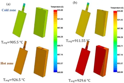
Figure 4.6 The model’s temperature distribution at the surface of the coupons and around the coupons for the case of without cathodic protection (a) and with cathodic protection (b) at non-isothermal condition of 800-950°C ...78

Figure 4.7 The corrosion current density distribution at the coupons without (a) and with Mg (b) introduced into the salt solution at the control temperature of 800-950°C and the amount of Mg of 1.15 mol% ...79

(15)

xiv

Figure 4.9 The effect of porous layer porosity on the corrosion rate distributions

at both cold and hot zones for the case with 1.15% Mg at non-isothermal condition (800-950 ℃). ...81

Figure 4.10 The effect of porous layer porosity on the corrosion rate at both cold zone and hot zone for the cases (a) without Mg and (b) with 1.15% Mg at non-isothermal case (800-950 °C) ...82

Figure 4.11 The effect of porous layer thickness on the corrosion rate at both cold zone and hot zone for the cases (a) without Mg and (b) with 1.15% Mg at non-isothermal case (800-950 °C) ...83

Figure 5.1 Example of IR_m corrected cell voltage (Em) vs. time for a 50-hour infusion of 64 ppm 2,6-DAT at 0.2 A/cm2_{into a 0.4 mg/cm}2_{Pt/C cathode catalyst loading...87}

Figure 5.2 Example of IR_m corrected cell voltage (Em) vs. time for a 50-hour infusion of 64 ppm 2,6-DAT at 0.2 A/cm2 into a 0.4 mg/cm2 Pt/C cathode catalyst loading...90

Figure 5.3 Corrected cell voltage, ΔE_m, for different model compounds (64 ppm) for 0.4 mg/cm2_{catalyst loading. The symbols are the experimental data and the lines are the model} prediction ...97

Figure 5.4 Parameters obtained by fitting the model to the experimental data at 30-hour, 0.4 mg/cm2 cathode catalyst loading at 64 ppm for four organic compounds (a) the rate of catalyst poisoning and recovery during contamination (γ_cc) and recovery (γ_cr), (b) the fraction of sites poisoned during contamination (1) and recovery (2) ...98

Figure 5.5 a) ΔE_m for different concentrations and infusion times of 2,6-DAT. The symbols are the experimental data and the lines are the model prediction. b) The contribution of kinetic and ohmic loss during the contamination and the recovery for the case of 256 ppm. The inset shows the contribution from each of the kinetic contamination (i.e., catalyst, and ionomer) to the voltage loss for the case of 256 ppm for 0.4 mg/cm2 catalyst loading ...100

Figure 5.6 ΔE_m for different catalyst loadings at 30-hour infusion time and 64 ppm 2,6-DAT ...102

Figure 5.7 The fraction of sites poisoned during the contamination time (1) for 2,6-DAT. The symbols correspond to the experimental conditions, given in Table 7.1 and the dotted line is the empirical fit to these parameter values (Equation 7-12) ...104

(16)

xv

Figure 5.9 The rate of ionomer poisoning during contamination γ_𝑖𝑐with 2,6-DAT. The symbols correspond to the experimental conditions, given in Table I and the dotted line is

the empirical fit to these parameter values (Equation 17-4) ...106

Figure 5.10 The fraction of sites poisoned during recovery (θ2) with 2,6-DAT. The symbols correspond to the experimental conditions, given in Table I and the dotted line is the empirical fit to these parameter values (Equation 7.15) ...107

Figure 5.11 The rate of catalyst recovery during the recovery with 2,6-DAT. The symbols correspond to the experimental conditions, given in Table 7.1 and the dotted line is the empirical fit to these parameter values (Equation 7-16) ...108

Figure 5.12 The rate of ionomer recovery during recovery (γ𝑖𝑟) with 2,6-DAT. The symbols correspond to the experimental conditions, given in Table 7.1 and the dotted line is the empirical fit to these parameter values (Equation 7-17) ...108

Figure 5.13 The fraction of contamination in the ionomer at steady state (𝑦₂) for 2,6-DAT. The symbols correspond to the experimental conditions, given in Table I and the dotted line is the empirical fit to these parameter values (Equation 7-18) ...109

Figure A.1 Schematic of a thermosiphon equipped in a furnace ...119

Figure A.2 Major components of thermosiphon ...120

Figure A.3 SEM analysis of Haynes 230 before corrosion testing (a), and after 100 hours corrosion testing (b) ...124

Figure A.4 (a) SEM cross-section image of Haynes 230 after 100 hours in KCl-MgCl2 at 850°C (a), and results of EDS linescan (the last 2 - 4 EDS points of the linescans may be of the mounting material) (b) ...125

Figure B.1 Anodic exchange current density as a function of temperature ...132

Figure B.2 Cathodic exchange current density as a function of temperature ...133

Figure B.3 Mg exchange current density as a function of temperature ...134

Figure C.1 Overall STAR-CD system structure ...135

(17)

xvi

LIST OF SYMBOLS

𝑎 : Active surface area of catalyst per volume (cm-1)

𝑎₀: Active surface area of catalyst per volume before contamination (cm-1)

𝐶_𝑂₂: Concentration of oxygenin the catalyst layer (mol cm-3₎

C_𝐻+_{: Concentration of proton in the catalyst layer (mol cm}-3₎

C_𝐻+_,0: Initial concentration of proton for baseline (mol cm-3)

𝐶_𝑖 : Concentration of species i in the bulk, (mol m-3₎

𝐶_𝑖∗ : Concentration of species i at the surface, (mol m-3₎

𝐶_𝑖𝑟𝑒𝑓 : Reference concentration of species i, 1.0 mol m-3_.

𝐷𝑒𝑓𝑓_{: Effective diffusion coefficients of reactant salts in grain boundary pores}

(m2 s-1

𝐷𝑖 : Diffusion coefficients of reactant i, in the bulk salts (m2 s-1)

𝐸 : Temperature and concentration corrected standard potentials (V)

𝐸0_{: Temperature corrected standard potential (V)}

Eeq: Open circuit potential (V)

E_m: IRm corrected voltage (V)

𝐹 : Faraday constant, (96,485 C mol-1₎

𝑖 : Current density, (A m-2)

𝑖0 : Exchange current density, (A m-2)

(18)

xvii

i_avg : Average corrosion current density at the surface of the coupon, (A m-2)

I : Current density (A cm-2)

Ni : Flux of a solute species i, (mol m-2_s-1₎

n : Number of electrons transferred in electrode reaction

𝑅₀: Ionomer resistance before contamination (ohm)

Ri : Ionomer specific resistance (ohm cm2)

Rm: Membrane specific resistance (ohm cm2)

R : Gas constant, (8.314 J mol-1 K-1)

t: Time (h)

T: Temperature, (K)

𝑥 : x-position, (m)

𝑌 : Mass fraction

Greek

α_𝑎,𝑐= transfer coeffcients

1

β: Tafel slpoe

γcc: Rate of catalyst poisoning (h-1)

γcr: Rate of catalyst recovery (h-1)

γic: Rate of ionomer poisoning (h-1)

γ_ir: Rate of ionomer recovery (h-1)

𝛿 : Porous layer thickness, (m)

𝜂 : Metal surface overpotential, (V)

ηa : Activation overpotentials of anode (V)

(19)

xviii 𝜅 : Thermal conductivity, (W K-1m-1)

𝜇 : Dynamic viscosity, (kg m-1s-1)

𝜌 : Density, (g m-3₎

θ: Number of active platinum sites loss

θ1: Fractional loss of catalyst sites after steady state contamination (i. e. , t → ∞)

θ2: Fractional loss of catalyst sites after steady state recovery (i. e. , t → ∞)

σ: Effective inomer conductivity (ohm-1cm-1)

σ₀: Inomer conductivity before contamination (ohm-1cm-1)

σ_𝑚: Membrane conductivity (ohm-1cm-1),

φ : TOC per amount of Pt at the catalyst layer (ppm mgPt-1)

𝜏 : Porous layer tortuosity

(20)

xix

LIST OF ABBREVIATIONS

ANL ... Argonne National Laboratory

BOP ... Balance of Plant

BzOH ... Benzyl Alcohol

CAE... Computer-Aided Engineering

CP ... Cathodic Protection

Cr... Chromium

CSP ... Concentration Solar Power

DGMEA ... Diethylene Glycol Monoethyl Ether

DGMEE ... Diethylene Glycol Monoethyl Ether Acetate

DOE ... Department of Energy

2,6-DAT ... 2,6 Diaminotoluene

EDS ... Energy Dispersive Spectroscopy

FV ... Finite Volume

H2 ...Hydrogen

(21)

xx

Mg ... Magnesium

NASA ... National Aeronautic and Space Administration

Ni... Nickel

O2 ... Oxygen

PEMFC ... Polymer Electrolyte Membrane Fuel Cell

SRNL ... Savannah River National Laboratory

TES ... Thermal Energy Storage

(22)

1

CHAPTER 1. INTRODUCTION

1.1 Clean Energy Technologies

The increasing the demand for energy, energy security and the need to minimize the

impact on the environment related to energy production are all major incentives for the

research and development of alternative energy technologies. There are several clean

energy sources that can alleviate fossil fuel shortages and environmental pollutant.

Examples of clean energy technologies that, one can refer to are concentrating solar power

(CSP) plants, and polymer electrolyte membrane fuel cells (PEMFCs).

For electricity generation on a large commercial scale, CSP has the potential to be a

highly economical conversion process. The conversion of sunlight to electricity, is one of

the leading candidates among clean energy technologies. Solar energy has enormous

advantages over other sources of energy because it is free, abundant, inexhaustible and

clean. Another important alternative source of clean energy is the use of hydrogen in

PEMFC fuel cells for both transportation and stationary applications. The extraordinary

environmental quality and high efficiency of PEMFCs make them a potential alternative

energy source.

Despite fundamental innovations that have advanced commercialization of these two

technologies, , many technical hurdles still need to be overcome to lower cost and achieve

(23)

2

Many clean energy programs have integrated a strong focus on electrochemistry due to

the high efficiencies that can be achieved by electrochemical reactions. The high

efficiencies of electrochemical processes are due to the direct relationship between

electrochemical energy and Gibbs energy from fundamental thermodynamics. Mechanical

systems used in energy applications such as turbines are limited by Carnot efficiency,

where electrochemical systems are only limited by the kinetics of the electrochemical

reaction and ohmic losses in the electrolyte. Corrosion mechanisms are also an

electrochemical phenomena that are important to understand and mitigate to prolong the

lifetime for clean energy systems. All of these aspects make electrochemical engineering

vital to further development of clean energy technologies [1].

In this work electrochemistry is used to improve the lifetime of these two clean energy

technologies. In the first part of this dissertation the corrosion problem in the CSP plant

are discussed, followed by a mathematical model development that include thermal

gradients and fluid flow to predict corrosion rates and mechanisms observed in the state of

the art molten salt heat transfer systems of CSP plants. The second part of the study is

devoted to identify the performance loss and recovery of a PEM fuel cell due to Balance

of Plant (BOP) materials contaminations via a combination of experimental data and

mathematical models.

1.2 Concentrated Solar Power (CSP) Systems

Diminishing fossil fuel reserves and increasing effects of anthropogenic climate change

due to greenhouse gas emissions have led to an unprecedented global interest in renewable

(24)

3

system has become one of the emerging technologies in the world. The defining aspect of

CSP is that it captures and concentrates solar radiation to provide the heat required to

generate electricity, rather than using fossil fuels or nuclear reactions. Another attribute of

CSP plants is that they can be equipped with a thermal energy storage system in order to

generate electricity even when the sky is cloudy or after sunset.

In general, CSP systems convert solar radiation into thermal energy by focusing the

sun's rays onto a central area called a receiver. The heat transfer fluid (HTF) inside the

receiver is heated by absorption of the radiation and is pumped through the receiver pipes to

deliver the thermal energy to a heat exchanger integrated with a steam turbine to generate

power. The processes occurring in CSP systems is illustrated in Figure 1.1. CSP systems

are early in their adoption, but have already begun commercialization. Today, there are 80

operational CSP plants around the world, mainly in the United States and Spain, with 1.9

GW of total capacity. Another 23 are under construction in India, China, Australia, and

South Africa, among other places [3]. As experience is gained with CSP systems and as

R&D advances, plants will get bigger, mass production of components will occur and costs

will come down with increased competition between CSP integrators.[4]. The U.S.

Department of Energy (DOE) target is to make unsubsidized solar energy cost competitive

with other forms of energy on the grid by the end of the decade. Figure 1.2 shows the

breakdown of CSP systems cost. It is projected that CSP systems need to be able to produce

energy with a cost of $0.06/kWh when they are scaled up and implemented on a large scale.

To reach these targets, it is generally believed that temperatures of the HTFs will need to

be high enough to drive an advanced Brayton cycle or Rankine cycle with superheated

(25)

4

CSP plants, reduce the cost of the thermal storage system (as a smaller storage volume is

needed for a given amount of energy storage) and achieve higher thermal-to-electric

efficiencies.

It is projected that average operating temperatures near 750°C with local hot spots up

to 850 °C would be needed to make these systems viable and achieve energy price goals.

To make this system feasible, HTFs that can operate at these temperatures for long periods

of time without significant degradation reaction of either the HFT or the materials of

construction for the system are required.

Figure 1.1. Schematic of a CSP plant [5].

A variety of HTFs which may be used in CSP systems have been considered and

researched, including six groups: gases (air, helium and super critical CO2), water/steam,

thermal oils, organic fluids, molten salts and liquid metals. Table 1.1 summarizes the

respective advantages and drawbacks of the different groups of HTFs that can be employed

(26)

5

Table 1.1. Advantages and disadvantages of the different groups of HTFs for CSP systems [6].

Air, helium and super critical

Water/steam Thermal oils Organic fluids Molten salts Liquid metals

Thermophysical properties

Low dynamic viscosity and high efficiencies. High operating

temperatures (above 700 °C). Impossibility of thermal storage, high pumping power and low thermal

conductivity.

Low dynamic viscosity (similar to air), non-expensive Rankine direct cycle. Limited operating temperatures (600 °C), impossibility of thermal storage and high pressure required.

Constant thermal conductivity over a wide range of temperatures and high efficiencies at small scales. Thermal

stability only up to 400 °C, low heat capacity, high pumping power

Low viscosity and high heat capacity. Low thermal

conductivity and limited temperature range (up to 393 °C).

Good thermal stability up to 600 °C, low viscosity and vapour pressure. Possibility of direct thermal storage. With new mixtures

temperatures of 800 e900 °C could be achieved, but with the drawback of a too high melting point (400 °C).

Large temperature range (above 1000 °C for most of the candidates) and thermal stability at high temperatures, high thermal conductivities, heat fluxes and efficiencies.

Possibility of thermal storage with some candidates.

Corrosion rate High oxidation rates at high temperatures, better

compatibility with less noble metals.

Corrosion starts at 300 °C and increases at high

temperatures.

No information regarding compatibility with materials is available in the literature.

Big corrosion issues at temperatures higher than 600 °C. Better compatibility with LiNaK mixtures.

Big corrosion issues at high temperatures for the heavy metals and fusible metals group Cost and availability High availability and zero costs. Low

availability in regions

characterized by high solar radiation rates.

Relatively high costs (between 3 and 5 USD/Kg).

High costs (100 USD/Kg).

Low costs but problems for meeting the demand of nitrate/nitrite based salts

(27)

6

Air and water are no longer considered as viable options. Air increases in volume when

heated and requires larger heat exchanger sizes for efficient heat transfer, which also

greatly increases the capital cost of the heat exchanger [7]. Water also can prove unstable

and difficult to manage at high temperature/high pressure situations. Thermal oils have

been a preferred heat transfer fluid for CSP developers designing low to intermediate

temperature CSP systems to get around the high pressure issue. The problem with thermal

oils is that the hydrocarbons break down when heated to 400 °C. and limit the maximum

operating temperature for parabolic troughs [8]. Liquid metals have been used as heat

transfer fluids in nuclear reactors since the 1940s and are currently being studied for use in

solar thermal systems as HTFs and thermal energy storage media. Although liquid metals

have not been used in commercial CSP applications until now, they have several promising

properties including extensive operating temperature range, low viscosity and efficient heat

transfer characteristics. The issue with liquid metal is that the cost is higher than that of

molten-salt or water/steam HTFs. Also, heat capacities of liquid metals are low relative to

commercial nitrate/nitrite based salts and hence they are less favorable to be used as

thermal energy storage media [9].

Molten salts proposed for use with high temperature Brayton and superheated Rankine

cycles are usually molten halides due to their good heat transfer properties. They can make

excellent heat transfer fluids in high temperature applications (260°C - 1400°C) because

of their high melting points, stability at high temperatures, and low viscosities. The size of

pipes and other equipment used for molten salts together with the pumping power required

(28)

7

The wall thicknesses required in using molten salts are also much smaller than those

required in high-pressure steam systems operating near the same temperatures [10].

Figure 1.2. The breakdown of CSP systems cost [11].

Certain molten salts can serve as energy storage mediums. Their high melting

temperatures and high thermal capacitances make it so they retain heat for periods longer

than 24 hours. They also have high energy densities which reduces the amount of molten

salt needed in applications normally carried out by traditional working fluids. Their ability

to store this heat energy allows electric energy at any time of the day [12].

The main disadvantage to using molten salts is that they can be highly corrosive,

especially at high temperatures. Therefore, piping, heat exchangers, pump heads, and other

components in CSP systems that come in contact with the molten salt are expected to face

(29)

8

1.3 Polymer Electrolyte Membrane Fuel Cell (PEMFC)

Proton exchange membrane fuel cells (PEMFCs) are considered to be a promising

technology for clean and efficient power generation in the twenty-first century. Their high

efficiency and zero emission have made them a prime candidate for powering the next

generation of electric vehicles [14]. Typical fuel cells operate at a voltage ranging from 0.6

– 0.8 V, and produce a current per active area (current density) of 0.2 to 1.0 A/cm2_{. A}

PEMFC consists of a negatively charged electrode (anode), a positively charged electrode

(cathode), and an electrolyte membrane. Hydrogen is oxidized on the anode and oxygen is

reduced on the cathode. Protons are transported from the anode to the cathode through the

electrolyte membrane, and the electrons are carried to the cathode over the external circuit.

The electrons are transported through conductive materials to travel to the load when

needed. On the cathode-side, oxygen reacts with protons and electrons forming water and

producing heat. Both, the anode and cathode, contain a catalyst to create electricity from

the electrochemical process as shown in Figure 1.3.

(30)

9

The conversion of the chemical energy of the reactants to electrical energy, heat and

liquid water occurs in the catalyst layers, which have a thickness in the range of 5 to 30

microns (μm). A typical PEM fuel cell has the following reactions:

Anode: H2 → 2H++ 2e−

Cathode : 1₂O₂+ 2H++ 2e− → H₂O

Overall: H₂+ 1

2O2 → H2O

1-1

1-2

1-3

Within the fuel cell, in addition to this chemical reaction, several coupled processes take

place at the same time, including the diffusion of reactants across the electrodes, diffusion

of protons across the membrane, heat generation and removal, water production at the

cathode, and water transport through and out of the fuel cell. The rates of the reaction and

these transport processes determine the dynamics of the fuel cell. These processes are

dependent on the quality of the membrane-electrode assembly (MEA), flow field designs,

and operating conditions (reactant flow rates, temperature, pressure etc.), all of which

affect the overall performance of the fuel cell and thus are important aspects to consider in

fuel cell design and operation.

In order to make fuel cell systems as commercially competitive as possible, as much

cost as possible needs to be removed from system components without sacrificing

performance and durability. Fuel cell durability requirements limit the performance loss to

a few tens of mVs over required lifetimes (1000s of hours). As fuel cell systems suffer

from performance loss due to factors such as potential cycling, start/stop and idling

conditions, there is very little tolerance for additional losses such as those due to

(31)

10

systems requires a level of understanding of potential contaminants from system

components that does not currently exist.

1.4 Dissertation Outline

As mentioned earlier, this dissertation is focused on two projects. The first six chapters

are focused on the first project and the last chapter addresses the second project. The

objective of first project is to create a comprehensive mathematical model including

thermal gradients and fluid flow to predict corrosion rates and mechanisms observed in

state of the art molten salt heat transfer systems. Chapter 1 introduces the importance of

the dissertation. It is generally believed that temperatures of heat transfer fluids (HTFs)

will need to be higher than 750 °C to drive an advanced Bryton cycle or Rankine cycle

with superheated steam to reach this target. To make this system technically feasible, HTFs

need to be developed that can operate at these temperatures for long periods of time without

significant degradation of either the HTFs or materials of construction for the system.

Decreasing materials’ corrosion will lower system maintenance costs due to less frequent

component failure and replacement. Improvements in materials’ durability will be

achieved by creating a comprehensive model that will allow identification of critical

parameters of corrosion mechanisms. While material durability studies have been

conducted for lower temperature HTFs that are common in industry, detailed

characterizations of molten salt systems capable of high temperature operation at

temperatures routinely exceeding 750°C have either not been performed or not been

extensive. The corrosion management strategies employed with higher temperature salts is

often drastically different when compared to those for the lower temperature nitrate salts

(32)

11

higher temperatures, activity gradient driven mass transfer and thermal gradient driven

mass transfer are often dominant, especially in many chloride and fluoride salt systems that

are among the most promising HOT HTFs. This research will characterize corrosion and

material degradation at these conditions and compare corrosion rates and mechanisms with

state-of-the-art systems.

Chapter 2 presents a literature review of the corrosion, specifically current research in

corrosion at high temperature molten salt systems and cathodic protection. Chapter 3

develops a corrosion model that allows reliable simulation of the processes under realistic

conditions that can help to identify the critical parameters of corrosion and improve the

material durability. Finally in Chapter 4, the previously reported corrosion model is

developed under magnesium (Mg) cathodic protection.

For the second project of the dissertation, the purpose is to identify the performance loss

and recovery of a fuel cell due to contaminants arising from Balance of Plant (BOP)

components via a combination of experimental data and mathematical models. An analysis

procedure was developed to quantify the various potential losses caused by contaminants

during both fuel cell contamination and recovery operations. These important impacts of

contamination are considered, which are the adsorption onto the Pt surface (kinetic losses)

and ion exchange with the membrane and ionomer in the catalyst layer. Chapter 5 presents

a literature review in addition to the experimental procedure and model development for

(33)

12

CHAPTER 2. LITERATURE REVIEW

2.1 Concentrated Solar Power Plant (CSP)

The first CSP plant (1982-1988) in California, US used water/steam systems as a heat

transfer fluid. Its six-year test and power production program proved that the technology

operates reliably and has both very low environmental impact and high public acceptance.

There were, however, two key disadvantages to the water/steam system at this plant. First,

the receiver was directly coupled with the turbine, causing the turbine to drop offline each

time a cloud came by, and second, the oil/rock thermal storage system was not efficient

because of thermodynamic losses. In parallel with testing of this plant, a series of studies

funded by the U.S. Department of Energy and industry examined advanced power tower

concepts using single-phase receiver fluids [16]. Molten salts have been studied for their

possibility of high working temperatures, low melting points, moderate density, high heat

capacity, and high thermal conductivity, in addition to long term thermal stability (or

chemical stability with less corrosion to containers) and low cost [17].

2.2 Molten Salt Applications in CSP Plant

The primary molten salt candidate was a binary mixture of 60% sodium nitrate and 40%

potassium nitrate (Solar Salt). The primary advantages of molten nitrate salt as the heat

transfer fluid for a solar power tower plant include a lower operating pressure and better

(34)

13

This translates into a smaller, more efficient, and lower cost receiver and support tower

[16]. Solar Salt has a thermal stability (below 600 °C) and a relatively high melting point

(220 °C). A new heat transfer fluid called Hitec, which is a ternary salt mixture of 53%

KNO3, 7 % NaNO3 and 40% NaNO2, has been considered to replace the Solar Salt because

of its low freezing point of 142 °C [18]. Hitec is thermally stable at temperatures up to 454

°C, and may be used at temperature up to 538 °C for a short period [19]. A modified

version, Hitec XL, is a mixture of 48 % Ca (NO3)2, 7% NaNO3 and 45% KNO3 which

melts at about 133 °C and may be used at a temperature up to 500 °C [18]. Different

compositions of Ca(NO3)2/ NaNO3/ KNO3 have been identified in the open literature as

eutectic salts [18, 20]. The ternary eutectic salt with composition of 44% Ca(NO3)2/ 12%

NaNO3, 44% KNO3 melts at 127.6 °C and its thermal stability is good at up to 622 °C [20].

It is proposed to replace molten-nitrate-salt coolant systems with molten-fluoride-salt

coolant systems and thus make it possible to increase peak salt coolant temperatures from

565 °C to between 700 °C and 850 °C. Increasing the peak coolant temperatures and using

a higher temperature closed-Brayton-power cycle have the potential to increase

heat-to-electricity efficiency by 20–30% with an equivalent reduction in capital costs [21].

Molten fluoride salts have been used on a large industrial scale for a century. Since the

1890s, essentially all aluminum has been produced by the Hall process which used

sodium-aluminum-fluoride-salt at 1000°C in a graphite-lined bath. In the 1950s, the United States

launched a large program to develop a nuclear-powered aircraft by using molten salt

reactors (MSRs) were to provide the very high- temperature heat source, with the heat

transferred to a jet engine via an intermediate heat-transport loop. In the 1960s and 1970s,

(35)

14

for these applications because of their high-temperature heat transfer and nuclear

characteristics [21]. Several types of molten fluoride and chloride salts, including LiF-BeF2

(also known as FLiBe [67-33 mol%]), LiF-NaF-KF (also known as FLiNaK [46.5-11.5-42

mol%]), and KCl-MgCl2 (67-33 mol%), have been investigated recently by several

Japanese and U. S. groups (LiF-BeF2 and LiF-NaF-KF) and by the University of Wisconsin

(LiF-NaF-KF and KCl-MgCl2) in support of fusion reactor and VHTR reactor concepts,

respectively. At operating temperatures, these salts have heat transfer properties similar to

those of water. However, the boiling points are above 1000 °C, which allows low-pressure

operations [22]. Table 2.1 presents a summary of the properties of molten halide salts for

using in CSP plants. Certain factors in this table, such as melting point and vapor pressure,

can be viewed as stand-alone parameters for screening candidates [23]. In the area of

nuclear energy systems, molten choloride salts are also being considered as heat transport

fluids to transfer high temperature process that from nuclear reactors to power chemical

plants. Electrochemical reprocessing of used metallic fuel is performed routinely in molten

LiCl-KCl electrolyte. Molten NaCl-KCl-MgCl2 salt was used in reprocessing of the liquid

metal fuel at Brookhaven National Laboratory in the 1950s as part of the Liquid Metal

Reactor Experiment. Free energy of formation vs temperature diagrams constructed for

chlorides show that alkali chlorides and alkaline earth chlorides are more

thermodynamically favored than the transition metal chlorides [24]. Williams discussed

the influence of the price of the components with different salt mixtures [23]. His

conclusions determined that magnesium chlorides are the least expensive of all, while

fluorides, fluoroborates and Li-containing mixtures increase the price of the coolant. Table

(36)

15

standpoint of the CSP plant, it is important to select a salt that possesses good heat transfer

characteristics, is relatively easy to handle, and not prohibitively expensive. Based on the

above issues it was decided that most of the experiments be performed for this project using

68%KCl-32%MgCl2 (mol%), with a couple tests utilizing FLiNaK salt for comparison

purposes. KCl-MgCl2 has less heat transfer properties, in comparison to the FLiNaK

molten salt, but it is one of the most inexpensive molten halide salts.

2.3 Super-alloys for CSP Plants

The development of the CSP plant much depends on the progress in creating such

structural materials that should meet a number of special requirements:

- A high corrosion resistance of molten salt melts;

- Adequate high-temperature strength;

- Good manufacturability (ability to be deformed, machined, welded, etc.).

The corrosive impact on these factors is significant in most situations, and may be

critical in some. In general, for structural materials, corrosion resistance is not the primary

criterion for selection. In most cases, for the applications described above, the mechanical

properties are the major needs. Obviously, this usually means strength (rupture strength,

creep strength, toughness) at the required service temperature. Since in all cases the

systems have to be fabricated at ambient temperature, and in normal operation will need to

be cooled to ambient temperature several times during their service lives, there will also be

some mechanical property requirements for low temperatures: the usual minimum

(37)

16

Table 2.1 Thermophysical properties of some molten salts compositions [23]. Heat-transfer properties at 700 ºC

Salt Formul

a Weight (g/mol)

Melting point

(ºC)

900ºC vapor pressure (mm Hg)

ρ, density (g/cm3₎

ρ Cp,

volumetric heat capacity

(cal/cm3 ºC)

μ, viscosity (cP)

k, thermal conductivity

(W/m K)

LiF-NaF-KF 41.3 454 ~ 0.7 2.02 0.91 2.9 0.92

NaF-ZrF4 92.7 500 5 3.14 0.88 5.1 0.49

KF-ZrF4 103.9 390 1.2 2.80 0.70 < 5.1 0.45

LiF-NaF-ZrF4 84.2 436 ~ 5 2.92 0.86 6.9 0.53

LiCl-KCl 55.5 355 5.8 1.52 0.435 1.15 0.42

LiCl-RbCl 75.4 313 -- 1.88 0.40 1.30 0.36

NaCl-MgCl2 73.7 445 < 2.5 1.68 0.44 1.36 0.50

KCl-MgCl2 81.4 426 < 2.0 1.66 0.46 1.4 0.4

NaF-NaBF4 104.4 385 9500 1.75 0.63 0.9 0.4

KF-KBF4 109.0 460 100 1.70 0.53 0.9 0.38

(38)

17

Table 2.2 Estimated raw material costs for various salt mixtures [23].

Salt Composition

(mol %)

Composition (wt %)

Raw material cost ($/kg–salt mixture)

Cost/volume ($/L at 700ºC)

KCl-MgCl2 68-32 62-38 0.21 0.35

NaCl-MgCl2 58-42 46-54 0.25 0.42

NaCl-KCl-MgCl2 20-20-60 14-18-68 0.28 0.50

LiCl-KCl-MgCl2 9-63-28 5-61-34 0.74 1.13

KF-KBF4 25-75 13-87 3.68 6.26

LiCl-KCl-MgCl2 55-40-5 40.5-51.5-8 4.52 7.01

LiCl-KCl 59.5-40.5 45.5-54.5 5.07 7.71

NaF-NaBF4 8-92 3-97 4.88 8.55

NaF-ZrF4 59.5-40.5 27-73 4.02 12.63

KF-ZrF4 58-42 32.5-67.5 4.85 13.58

(39)

18

The selected materials must be fabricable to the extent required to manufacture the

system; but there is often a further requirement in the fabricability of the materials since it

is likely that during service repairs and replacements may be necessary.

For higher temperature applications, it is necessary to produce alloys with higher

intrinsic oxidation resistance. Developments along these lines had begun for quite different

reasons in the late 1920s, when a series of alloys were developed, primarily for electric

resistance heater applications, which relied on the growth of a protective Cr2O3 ‘chromia’

scale. These alloys were nickel or cobalt based, and when the first gas turbines were

developed for aviation purposes these were selected for the hot components [25].

A National Aeronautic and Space Administration (NASA) study determined that the

tendency for common alloying constituents to corrode in molten fluoride salts increased in

the following order: Ni, Co, Fe, Cr, Al. This is supported by Gibb’s free energy of

formation of various fluorides [26].

The present-day corrosion-resistant nickel alloys, which can be well deformed and

welded, belong to three main alloying systems: Ni-Mo, Ni-Cr, Ni-Cr-Mo. Simultaneous

alloying of nickel with chromium and molybdenum makes it possible to create

ultrahigh-resistance alloys in a wide range of corrosive active media of oxidation/reduction character.

Along with a high corrosion resistance, the alloys show an exceptional resistance to local

types of corrosion. Besides, these alloys are heat-resistant at high temperatures. They

combine high strength and plasticity from temperatures below zero to 1200°C. The effect

of mutual effect of chromium and molybdenum on the corrosion resistance of the alloy is

(40)

19

Haynes Alloy N was developed in the 1950s for molten salt service in the Aircraft

Nuclear Propulsion program. Conventional high temperature alloys containing about 20%

chromium proved susceptible to corrosion by the proposed molten salt heat transfer

medium. It was successfully used in the ORNL Molten Salt Reactor Experiment in the

1960s. Some variations of Alloy N, for example, adding titanium, (McCoy, et al., 1970)

were developed for easier weldability and better performance in the high radiation

environments of reactors [28].

The primary materials used while investigating corrosion in high temperature CSP

applications are: Haynes-230, Incoloy 800H, and Haynes NS 163. These alloys were

chosen over continued testing of different alloys because their mechanical properties are

much more suitable to sustained high temperature operation. Table 2.3 shows the

compositions of these different alloys.

Table 2.3. Compositions of super-alloys.

Alloy (wt%) Cr Mo W Al Ti Fe C Co Ni Mn V Si

Incoloy 800H 20.82 - - 0.54 0.52 46.3 0.07 0.04 30.69 0.49 - 0.33

Haynes 230 22.08 1.23 14.17 0.37 0.01 1.02 0.10 0.21 59.98 0.52 - 0.31

Haynes NS 163 27.71 0.27 - 0.17 1.33 21.24 0.092 40.66 8.06 0.22 0.05 0.20

As it is shown in Table 2.3 these super-alloys have a large Al and Cr component to aid

in the prevention of high temperature oxidation. As discussed earlier both Al and Cr are

(41)

20

2.4 Corrosion of Super-alloys in Molten Salt

Compatibility of molten salts with structural alloys centers on the potential for oxidation

of the structural metal from the elemental state to the corresponding fluorides or chlorides

with corresponding reduction of the oxidizing agent. Electrochemically, the molten

salt/metal surface interface is very similar to the aqueous solution/metal surface interface.

Many of the principles that apply to aqueous corrosion also apply to molten salt corrosion

such as anodic reactions leading to metal dissolution and cathodic reduction of an oxidant

[22]. The laws of electrochemistry and mechanisms of corrosion are comparable for

aqueous solutions and molten salts. According to Joseph R. Davis [29] the most common

mechanism is the oxidation of the metal to ions, similar to aqueous corrosion. For this

reason, molten salt corrosion has been identified as an intermediate from of corrosion

between molten metals and aqueous corrosion.

The corrosion of metals in molten salt can be well explained by a combination of anodic

dissolution of metal (𝑖𝑎) and cathodic reduction of oxidants (𝑖𝑐) under a mixed potential as

well as in aqueous solution. The polarization curve is schematically illustrated in Figure

2.1. The partial anodic current 𝑖_𝑎 and cathodic current 𝑖_𝑐 correspond to the metal

dissolution and the reduction of oxidants respectively in corrosion processes. They are

represented by broken curves in Figure 2.1. The rates of anodic reaction and cathodic

reaction must become equal at a corrosion potential 𝐸_{𝑐𝑜𝑟𝑟}. That is to say, the partial anodic

current and the partial cathodic current become equal in magnitude and opposite in

direction. And the value is designated the corrosion current, 𝑖_{𝑐𝑜𝑟𝑟}:

(42)

21

Generally, the anodic reaction of corrosion in a molten salt corresponds to the

dissolution of metals followed by the formation of metal oxides or salt films in the same

way in aqueous solution. On the contrary, the cathodic reaction of corrosion differs with

each molten salt and is much more complicated than the aqueous solution system [30].

The oxidation-reduction (corrosion) can occur by several processes in molten salt,

including: Uniform surface corrosion, differential solubility due to thermal gradients, and

galvanic corrosion.

Intrinsic corrosion (uniform surface corrosion) with molten salt as the reactant; this

mechanism pertains primarily to nitrates and nitrites, not to fluorides or chlorides [29].

According Ozeryanaya [31] the oxidation of metals by molten chlorides is an

electrochemical process of ion exchange between the metal and the salt:

𝑀 → 𝑀𝑛+_{+ 𝑛𝑒}−

𝑜𝑥 + 𝑛𝑒− _{→ 𝑟𝑒𝑑}

2-2

2-3

These reactions take under conditions close to equilibrium with respect to the salt

adjacent to the electrode. Even in the absence of oxidizing contaminants (oxygen, water,

etc.) the salt cations which can be reduced to the elemental state, or to a lower state, can

act as metal-depolarizers.

Corrosion by oxidizing contaminants in the molten salts (such as HF, HCl, H2O),

residual oxides of metals, or easily reducible ions, especially some polyvalent metal ions.

Impurities in the melt or in the gas phase control the corrosion/oxidation potential of the

(43)

22

Figure 2.1 Schematic polarization curves for the metallic corrosion system. 𝑖_𝑎 and 𝑖_𝑐 indicate the partial anodic and cathodic currents respectively [30].

Differential solubility due to thermal gradients (between hot and cold zones) in the

molten salt system with formation of a metal ion concentration cell that drives corrosion.

Thermal gradient in the melt can cause dissolution of metal at hot spots and metal

deposition at cooler spots. The result is very similar to aqueous galvanic corrosion [29].

Galvanic corrosion, wherein alloys with differing electromotive potentials are

maintained in electrical contact by the molten salt, is driving the oxidation of the anodic

material. According to Ozeryanaya [31] at high temperatures, not only the salt components

but also the container material can act as metal oxidizers. He showed the formation of metal

alloys through molten salts goes in a strictly defined direction: the more chemically active

metal M1 (electronegative) corrodes in the molten bath:

M₁ → M₁m+_{+ me} _2-4

The low-oxidizing-level ions M₁m+ of that metal transfer by convection towards the more

(44)

23

nM₁m+↔ (n − m)M₁+ m M₁n+ at n > m 2-5

The atoms of the active metal M1 formed in this way produce an alloy M1-M2 while the

M₁n+_{ions, reaching the surface of}_M

1, accelerate its corrosion:

(n − m)M1+ m M1n+ ↔ n M1m+ 2-6

For instance, the corrosion rate of a Cr specimen in molten NaCl at 900°C increases 30

times if an alundum crucible (inert with respect to the salt) is replaced by an iron crucible.

In the latter case Cr corrodes as:

Cr → Cr2+_{+ 2𝑒}− _2-7

while on the crucible surface the following reaction takes place:

3Cr2+ _{↔ 2 Cr}3+_{+ Cr}

𝑎𝑙𝑙𝑜𝑦 2-8

High temperature corrosion in molten salts often exhibits selective attack and internal

oxidation. As an example chromium depletion in iron-chromium-nickel alloy systems can

occur by the formation of a chromium compound at the surface and by the subsequent

removal of chromium from the matrix, leaving a depleted zone. Thus, the selectivity

removed species moved out, while vacancies moved inward and eventually form voids.

The voids tend to form at grain boundaries in most chromium- containing metals [29].

Figure 2.2 compares alloys high in nickel and chromium with and without exposure to

FLiNaK salt, held at 850°C for 500 hours. The images demonstrate coupons exposed to

the salt have significant weight loss along grain boundaries.

Corrosion of metals in fluoride salts was investigated for MSRs development as early

as 1950. Various alloys were tested in mixtures of LiF, BeF2, NaF, ZrF4, ThF4, NaBF4, etc.,

up to about 1088 K using static experiments, convection loops and in-pile surveillance

(45)

24

Figure 2.2 a) 10,000 magnification SEM image of Incoloy 800H held at 850˚C for 500 hours, no salt exposure, b) 250 magnification of Incoloy 800H held at 850˚C for 500 hours, FLiNaK exposure.

In most high temperature environments corrosion can be controlled by one of the

following mechanisms, (i) by the formation of a protective film, or [33] by the

establishment of a thermodynamic equilibrium between the material and the environment

[4]. Elements such as Cr, Al, and Si are added to alloys to promote the formation of

self-healing protective oxide films that act as diffusion barriers and prevent further rapid

oxidation in oxidizing environments such as air. Prevention of hot corrosion (sulfidation

and oxidation from molten salt deposits left from fuel impurities) in fossil fueled boilers

and turbines also rely on passive films of Cr and Al oxides present at the alloy surface [32].

Additionally, chemical additions to the fuel aid in removal corrosive salt slags [32]. Gas

turbines and boilers that burn fossil fuels use these corrosion prevention methods

extensively. Molten fluoride salt corrosion of most high temperature alloys however, is

fundamentally different from air oxidation and hot corrosion [6]. Unlike conventional

air/aqueous oxidation, the protective oxide films are soluble in molten fluoride salts or

otherwise unprotective [15]. The corrosion rate therefore depends on the thermodynamic

driving force and the kinetics of the various corrosion reactions [15]. In general, there are

Surface Cross-section

Cr Carbides

Grain triple point Cross-section

(46)

25

three driving forces for corrosion in molten fluorides: impurities, temperature gradients,

and activity gradients [34].

Several high temperature Fe-Ni-Cr and Ni-Cr alloys: Hastelloy-N, Hastelloy-X,

Haynes-230, Inconel-617, and Incoloy 800H, and a C/SiSiC ceramic were exposed to

molten FLiNaK with the goal of understanding the corrosion mechanisms and ranking

these materials for their suitability for molten fluoride salt heat exchanger and thermal

storage applications. The tests were performed at 850°C for 500 h in sealed graphite

crucibles under an argon cover gas. Corrosion was noted to occur predominantly from

dealloying of Cr from the alloys, an effect that was particularly pronounced at the grain

boundaries [34].

Inconel alloy 600 and certain stainless steels become magnetic after exposure to molten

fluoride salt. This magnetism is caused by the selective removal of the chromium and the

formation of a magnetic iron-nickel alloy covering the surface.

Molten salts consisting of chlorides are important but they have been studied less than

fluoride system. In general chloride salts attack steels very rapidly, with preferential attack

of the carbides. In chloride salts no protective oxide scale is formed on the nickel base

alloys. The attack of metal surfaces in pure sodium chloride has been observed at

temperatures above 600 °C.

In most cases with iron-nickel-chromium alloys, the corrosion takes the form of

intergranular attack. An increase of chromium in the alloy from 10% to 30% increases the

corrosion rate by a factor of seven. Thus, the intergranular attack is probably selective with

(47)

26

with diffusion of chromium from within the grain to the boundary layer, gradually

enlarging the cavity in the metal. The gross corrosive attack is probably caused by the free

chlorine, which is highly oxidizing material, attacking the highly active structure-sensitive

sites, such as dislocations and grain boundaries. Figure 2.3 shows an example of

intergranular corrosion of Ni-Cr-Fe alloy by molten chloride salt after 6 months at 870°C

[29].

Figure 2.3 An example of intergranular corrosion of Ni-Cr-Fe alloy by molten chloride salt after 6 months at 870°C [29].

2.5 Cathodic Protection

It is well known that cathodic protection (CP) can inhibit metal corrosion [35, 36].

Among the various corrosion control methods available, cathodic protection is a widely

used technique adopted to control the corrosion of the alloy by effecting a change in

potential from the natural corrosion potential (𝐸𝑐𝑜𝑟𝑟) to a protective potential in the

(48)

27

exposed to any electrolyte. Corrosion can be reduced to virtually zero, and a properly

maintained system will provide protection indefinitely.The first application of CP can be

traced back to 1824, when Sir Humphrey Davy, in a project financed by the British Navy,

succeeded in protecting copper sheathing against corrosion from seawater by the use of

iron anodes [37]. CP reduces the corrosion rate by cathodic polarization of a corroding

metal surface. Cathodic polarization reduces the rate of the half-cell reaction with an excess

of electrons. Metal structure can be cathodically protected by connection to a second metal,

called a sacrificial anode, which has a more active corrosion potential. The noblest structure

in this galvanic couple is cathodically polarized, while the active metal is anodically

dissolved. Magnesium, zinc and aluminum sacrificial anodes, provide long-term cathodic

protection [38]. Matson et.al [39] developed the experiments to determine the feasibility of

using cathodic protection to reduce the attack in the fluoride volatility process for recovery

of nuclear fuel at 650 °C. Their results show that CP would reduce the corrosion of

submerged Inor-8 components in fused fluoride salt systems by factor of 10. For the

KCl-MgCl2 molten salt system, metallic Mg was identified as a potential corrosion inhibitor

[40]. As it is the most electrochemically active metal, which corrodes so readily in some

environments that Mg and Mg alloys are purposely utilized as sacrificial anodes in

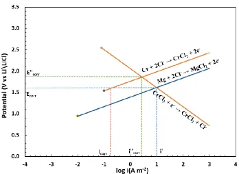
engineering applications [41]. Figure 2.4 shows the electrochemical equilibrium potential

for Mg going to MgCl2 and compares that to the potentials for other alloy components

going to their molten chlorides. This shows that the equilibrium potential is well below the

(49)

28

Figure 2.4 Electrochemical potential for alloy components and Mg corrosion inhibitor [40].

2.6 Modeling of High Temperature Corrosion

Corrosion predictive models are a very useful tool that can be used to determine

corrosion allowances, make predictions of facilities remaining life, and provide guidance

in corrosion management. For high temperature molten salt systems, it has been found that

Cr will be dealloyed primarily in high temperature regions where selective attack results in

the formation of voids [42]. If the chromium content in the depleted-zone is lower than a

critical level, it is then vulnerable to environmental corrosion, leading to inter-granular

attack [43], or intergranular stress corrosion cracking (IGSCC) [44]. For these reasons,

many studies have been devoted to correlating IGSCC to grain boundary characteristics

and to a quantitative evaluation of the dechromised zones by experimental analysis and

empirical or analytical computer modelling [44-46]. Thrvaldsson et al. [45] used the error

function solution of Fick’s second law for Cr diffusion, for Cr depleted zones adjacent to

(50)

29

approximation of the depleted zone morphology in the early stages of aging. A three

dimensional (3-D) modeling technique has been also developed to predict the Cr depletion

from grain boundaries in a Ni-Cr-Fe alloy (Inconel 690) [44]. In Anderko et al. [46] a grain

boundary microchemistry model has been developed that calculate the chromium and

molybdenum depletion profiles in the vicinity of grain boundaries. Their model could relate

the repassivation potential to the microchemistry and environmental conditions. The

literature models have been successful in predicting the Cr depletion profiles. However,

the corrosion model developed for nickel-based alloys in molten salts that considers the

fluid flows in the non-isothermal condition of CSP plants has not been fully defined. A

corrosion model reliably simulating the corrosion processes under realistic CSP plant

conditions can help identify critical corrosion parameters that can lead to improved

material durability. Combined CFD and electrochemical analysis of CSP plant heat transfer

systems can lead to predictions and insights on the interplay of thermal and concentration

gradients under convection. The coupling of the corrosion model with CFD can allow

predictions of local corrosion rates as functions of heat and mass transport in the local