Two-dimensional simulation of vortex points and tracer particles in
counterflowing He-II
E. Varga1,a, C. F. Barenghi2, Y. A. Sergeev3, and L. Skrbek1
1 Faculty of Mathematics and Physics, Charles University in Prague, Ke Karlovu 3, 121 16 Prague, Czech Republic 2 Joint Quantum Centre Durham-Newcastle, School of Mathematics and Statistics, Newcastle University, Newcastle upon
Tyne NE1 7RU, United Kingdom,
3 Joint Quantum Centre Durham-Newcastle, School of Mechanical and Systems Engineering, Newcastle University, New-castle upon Tyne NE1 7RU, United Kingdom,
Abstract. The article presents results obtained based on numerical simulation of two-dimensional vortex points and inertial tracer particles in two-component counterflowing superfluid He-II. In the low temperature limit (no normal fluid, no friction) our model would reduce to Onsager’s famous vortex gas. The flow of the nor-mal component of the He-II is assumed uniform, while the superfluid velocity field is induced by vortex points which model three-dimensional quantized vortex lines. Probability density functions of velocity and accelera-tion of tracer particles and superfluid velocity field are obtained. We find that tails of probability distribuaccelera-tions follow power-laws with various exponents, except in the case of sufficiently coarse-grained superfluid velocity field, where Gaussian shape is observed. The decay of the number of vortices is also studied, yielding results in agreement with Vinen’s phenomenological model of quantum turbulence.
1 Introduction
Liquid4He cooled below certain temperature (so-called λ-point, approx. 2.17 K at SVP) becomes superfluid and is called He-II. Properties of this liquid phase are strongly influenced by quantum-mechanical effects and are conve-niently, with sufficient accuracy, described by a two-fluid model. This model identifies two components within He-II – the superfluid component with zero viscosity that car-ries no entropy, and the viscous normal fluid component that carries all the entropy of the liquid. Due to quantum-mechanical constraints, the vorticity of the superfluid com-ponent cannot be arbitrary, as in classical viscous fluids, but is concentrated to thin topological defects of the size of the order of inter-atomic distance, usually imagined as lines, around which circulation is quantized in unitsκ ≈ 10−7m2 called quanta of circulation. Turbulence is possi-ble in both components. In the normal component it is as-sumed that the turbulence is essentially the same as in clas-sical viscous fluids. In the superfluid component, however, the turbulence takes the form of a complex tangle of vortex lines.
Turbulence in He-II has been extensively studied both experimentally and numerically for several decades. The numerical approach usually builds upon Schwarz’s model of quantized vortex lines as three-dimensional (3D) space curves [1]. Because of the 3D discretization required and the nonlocal character of the vortex-vortex interaction, such calculations are computationally expensive. The two di-mensional (2D) model here considered [2] is significantly simpler and idealized, as the space curves representing vor-tex lines are reduced to vorvor-tex points; at zero temperature
a e-mail:[email protected]
(T =0) the model would reduce to the famous vortex gas of Onsager.
From the physical point of view, the type of turbu-lence considered here is peculiar to superfluid4He and is known as thermal counterflow. In order to generate thermal counterflow experimentally, a heater is placed at the closed end of a channel. When power is supplied to this heater, the normal component of He-II starts to flow away from the heater, carrying with it all the entropy deposited by it. The superfluid component flows in the opposite direction towards the heater to maintain constant density and zero mass flux (that is,ρn+ρs=constant andρnvn+ρsvs=0). The superfluid and normal fluid velocities along the chan-nel are respectively [4]
vn= ˙ Q
ρS T, vs=− ˙ Qρn ρρsS T,
(1)
where ˙Qis the heater’s power per unit area (heat flux),ρs, ρnandρare the superfluid, normal fluid and total densities, respectively,S the specific entropy per unit mass, andvs, vn the superfluid and normal fluid velocities (positive ve-locities are in the direction away from the heater, negative towards it.)
Counterflow turbulence is usually characterized by the vortex line density,L, (defined as the quantized vortex length per unit volume), which is related to the counterflow veloc-ityw=|vn−vs|by Vinen’s phenomenological equation [3]
dL dt =c1
Bρn
2ρwL3/2−c22πκ L2, (2)
where B is the mutual friction coefficient andc1,c2 are parameters of order unity.
C
Owned by the authors, published by EDP Sciences, 2014
At given counterflow velocityw, this equation predicts a steady state valueLproportional tow2. Decaying solu-tions of equation (2) are found by settingw=0; we obtain:
L(t)= L0 1+c2κL0t/(2π)
≈ 2π
c2κt
fort→ ∞, (3)
whereL0is the initial condition att=0.
The article is structured as follows. The next section introduces the necessary equations used to run the numeri-cal simulations. The third section describes the simulations and the chosen parameters. The fourth section is dedicated to results, and the fifth concludes the paper.
2 Equations of motion
Letrdenote position on thexyplane. Letrjbe the location of the vortex point j = 1,· · ·N of (positive or negative) circulationκj. The superfluid velocity at rj is the sum of any applied superflowvextS and the superflow induced by other vorticesi=1,· · ·N(ij):
vs(rj)=vexts (rj)+ 1 2π
N
i=1,ij κi
ˆz×(rj−ri)
rj−ri2 , (4)
The vortex points j=1,· · ·Nmove such that Magnus and friction forces are in balance [1]:
drj
dt =vs(rj)+ακiˆz×(v ext
n −vs(ri))+α(vextn −vs(ri)), (5)
wherevextn is the imposed normal fluid velocity andα,α are known temperature-dependent mutual friction coeffi-cients.
In the absence of gravity, the equation of motion of a tracer particle located atrpis [5]
dup
dt =
1
τ(vn−up)+ 3 2ρ0
ρnD vn Dt +ρs
Dvs Dt
, (6)
where up = drp/dt is particle’s velocity, τ the viscous relaxation time, ρp the particle’s density, andρ0 = ρp + ρ/2. The assumptions behind equation (6) are discussed by Pooleet al.[5]; in particular the particle is smaller than any other relevant length scale and does not affect the flow (one-way coupling), the normal fluid’s flow around it is laminar (hence Stokes’s drag formula applies), and it does not interact with other particles. The substantial derivatives are defined as
Dvn
Dt =
∂vn
∂t +(vn· ∇)vn,
Dvs
Dt =
∂vs
∂t +(vs· ∇)vs. (7)
In the present work the normal fluid velocity is as-sumed to be uniform (constant in time and space),vextn =vn and particles are chosen to be neutrally buoyant,ρp = ρ. With these assumptions equation (6) reduces to
dup
dt =
1
τ(vn−up)+ρρsD vs
Dt . (8)
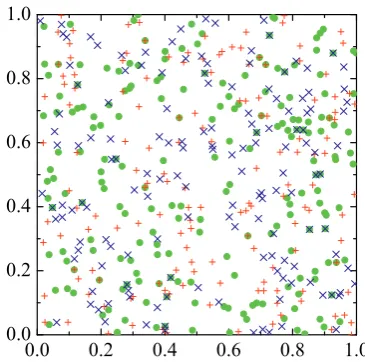
Fig. 1.A snapshot of vortices and particles in the computational domain. Red “+” symbols represent vortices with positive circu-lation and blue “x” symbols those of negative circucircu-lation. Green circles represent tracer particles.
Assuming that tracer particles are spheres of radiusa, the relaxation timeτ[5] isτ=2a2ρ
0/(9μn) whereμnis the viscosity of the normal fluid.
Equations (5) and (8) do not model all the behaviours than needs to be simulated. Firstly, it is known that when two vortex lines get sufficiently close to each other they reconnect [9, 10]. Since our model does not contain details at this microscopic level (which would require the use of the Gross-Pitaevskii equation), this effect needs to be ad-dressed algorithmically. The reconnection process cannot be ignored because the mutual friction force can push two vortices of opposing signs very close together. In 2D the reconnection algorithm is simple: when two vortices of op-posing signs approach each other (closer than an arbitrary reconnection length, see table 1), they annihilate, and, un-less we study the decay of turbulence, they are re-inserted back into the computational domain at random positions to maintain the statistical steady state.
Secondly, tracer particles can become trapped on vor-tices. To take particle trapping into account we implement the following algorithm: when a particle becomes closer to a vortex than an arbitrary trapping length (see table 1), we tag it as trapped and let it move as the vortex hereafter. We allow a trapped particle to become free (detrapping) if the vortex to which it was trapped undergoes a reconnection with a vortex of the opposite sign. Reducing the reconnec-tion distance by a factor of 100 did not alter the conclusion.
3 Numerical calculations
vortices) to experimentally known values taken from refer-ence [6].
All calculations used N = 300 vortices (150 positive and 150 negative) andNp =200 tracer particles. The vor-tices were initially (t = 0) set at random locations. The particles’s initial position was also random, with veloc-ity matchingvn. The system was evolved for one (dimen-sionless) time unit, sampling positions, velocities and ac-celerations of tracer particles periodically. Data sampled this way were treated as a single ensemble for calculat-ing statistics, so histograms of velocity or accelerations which we present represent time averages. In order to sam-ple the superfluid velocity field we set up a regular grid of 1000×1000 points where we evaluated velocity and La-grangian acceleration, that is, the substantial derivative of the superfluid velocity field defined by equation (7). Data were sampled 10 times during the calculation, and his-tograms were calculated from the entire ensemble. All he-lium fluid parameters (densities, specific entropy and mu-tual friction coefficients) were taken from Reference [11]. The parameters which we used are listed in table 1. An adaptive 4th order Runge-Kutta scheme was used for inte-grating the equations of motion in time.
A illustrative snapshot of the positions of vortices and particles in the computational domain is shown in figure 1.
4 Results
The most important statistical properties are the mean val-ues of the magnitudes of velocity and acceleration over the time evolution; these quantities are shown in figures 2 and 3 as functions of the imposed heat flux.
It is apparent from figures 2 that the free particles’ ve-locity closely follows that of the counterflowing normal fluid, while the velocity of trapped particles systematically exceeds that of the counterflowing superfluid. By construc-tion, the latter is also the velocity of the vortices. This dif-ference is probably due to the first mutual friction term in equation (5), which imparts to the vortices (and hence to the trapped particles) a motion in the direction transverse to the direction of the imposed counterflow. The result that the mean velocity of all particles is close to the mean ve-locity of trapped particles is probably due to the fact that, as a detrapping mechanism, 2D vortex reconnections is not effective enough – at any instant after an initial transient most particles in the simulations are trapped.
Mean acceleration magnitudes are shown in figure 3, averaged over all particles or separated as for velocities. This set of results allows direct comparison with exper-iments, for example, this quantity was measured by La Mantiaet al[6]. Experimental values from that work are included in the figure. The agreement with the experiment is rather poor, within an order of magnitude. A possible explanation for this discrepancy (besides the fact that our model is only 2D) is that experimental values are inferred from observed trajectories, whereas in our simulations, the instantaneous acceleration is calculated from the known positions and velocities of the vortices. Such quantity will be subject to strong fluctuations which, however, do not cancel out in the mean when calculating acceleration mag-nitudes.
Our data also allow for calculation of normalized his-tograms, or probability density functions (PDFs). PDFs of
Fig. 2.Mean velocity magnitudes of tracer particles calculated atT =1.75 K. Here the particles are separated into two groups: free and trapped particles. Mean values are taken over the two groups and over the entire ensemble as well. Black squares de-note magnitudes of velocity, averaged over all particles, green triangles over trapped particles only, and red circles over free par-ticles only. The upper black line is the imposed normal fluid ve-locity, the lower red line is the imposed superfluid velocity; both lines are calculated from equation (1).
.
Fig. 3.Mean magnitudes of accelerations of tracer particles. The particles are separated into groups as in figure 2. Green upwards-pointing triangles correspond to free particles, blue downwards pointing triangles to trapped particles, and red circles to average over all particles. Black squares represent experimental values from [6]. Temperature is 1.75 K.
transverse (to the mean direction of counterflow) compo-nent of velocity and acceleration for tracer and fluid par-ticles are in figures 4 – 7. In these plots, the xaxes are normalized by the standard deviation: numerical values are in table 2. For tracer particles’ PDFs, no distinction be-tween trapped or free particles was made. In all four cases, power-law tails are observed, as clearly visible in the insets of these figures.
For velocities of fluid particles, the obtained exponent of the power-law tail is consistent with the expected value of−3 [7]. It is worth noting that the inertial tracer particles are not found to faithfully follow the statistics of the fluid particles. However, it is possible that small size statistics for the tracer particles could be the reason.
Table 1.Parameters used in numerical simulations. The meaning of columns is as follows: at given temperatureT,Ddenotes the size of the computational box,Tt andU=D/Tt are the units of length, time and velocity, respectively;Qdenotes the heat flux supplied to
the counterflow heater;vn andvs stand for the counterflow-imposed velocities of the normal fluid and the superfluid;τis the viscous
relaxation time. In all cases, particle radius was set to be 5μm, reconnection lengthD/500 and trapping lengthD/500 + (particle radius).
T(K) D(m) Tt(s) U(m/s) Q(W/m2) vn(m/s) vs(m/s) τ(s)
1.65 1.264×10⁻³ 16.04 7.884×10⁻⁵ 490 6.105×10⁻³ −1.46×10⁻³ 9.34×10⁻⁴
1.75 1.732×10⁻³ 30.09 5.756×10⁻⁵ 414 3.519×10⁻³ −1.288×10⁻³ 9.38×10⁻⁴
1.75 1.237×10⁻³ 15.34 8.061×10⁻⁵ 590 5.015×10⁻³ −1.836×10⁻³ 9.38×10⁻⁴
1.75 1.212×10⁻³ 14.74 8.223×10⁻⁵ 608 5.168×10⁻³ −1.892×10⁻³ 9.38×10⁻⁴
1.75 1.074×10⁻³ 11.57 9.284×10⁻⁵ 691 5.873×10⁻³ −2.15×10⁻³ 9.38×10⁻⁴
Fig. 6.Probability distribution of the superfluid velocity com-ponent perpendicular to the mean counterflow, normalized by the standard deviation (see table 2). The figure contains 4 curves with colors and styles as in figure 4. The inset shows comparison with the predicted power law with the−3 exponent, in log-log plot.
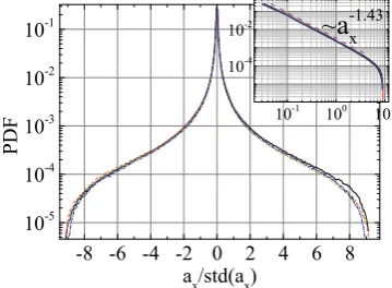
Fig. 7.Probability distribution of superfluid Lagrangian particle acceleration component perpendicular to the mean counterflow, normalized by the standard deviation (see table 2). The figure contains 4 curves as figure 6. The inset shows the same data on a log-log scale with a power law of fitted exponent−1.43.
The observed sharp cutoff in the fluid particles’ accel-erations, at around 9 standard deviations, is probably due to the fact that points where the acceleration is sampled do not get arbitrarily close to vortices.
The superfluid velocity field (velocities of the fluid par-ticles) are sampled on a regular square grid. This allows for coarse-graining of the velocity field, thus modelling the finite-size of a measurement region. Figure 8, with nu-merical values for standard deviations given in table 3, shows the progression of change of the PDF as the grid gets more and more coarse. The power-law tails disappear
Fig. 8.Probability distribution of coarse-grained superfluid ve-locity. The legend in the figure corresponds to the curves in order from top to bottom. The coarse-graining is accomplished by im-posing a coarser mesh on underlying mesh of 1000×1000 points where velocity is calculated and averaging the velocity in the cells of the coarser mesh. The last curve, 17×17, approximately cor-responds to coarse-graining on the scale of inter-vortex distance. The numbers in the legend show how many cells are in the coarse mesh. The temperature is 1.75 K and heater power is 608 W.
and the distributions assumes an approximately Gaussian form. Similar behaviour is observed in [12].
It is also possible to model the decay of turbulence by not reinserting back the vortices that annihilate. Fig-ure 9 shows the decay starting from three different num-bers of vortices at 1.65 K. Figure is kept in dimensionless time, because to fix the time scale vortex line density must be known. This can be inferred from the intended heater power, but since during the decay the heater is switched off, the choice would be arbitrary. All curves, however, have the same time scale. The curves are found to be in good agreement with Vinen’s decay (3).
5 Conclusions
We performed computer simulations of vortex points and tracer particles in a simple two-dimensional model of su-perfluid helium. We found that the mean particle velocity closely follows the velocity of either component of coun-terflowing He-II, depending on whether particles are trapped into vortices or not. The tracer particle accelerations are much higher than those observed in the experiments; this effect is probably caused by the 2D trapping and detrap-ping mechanisms which we used, and will require further attention.
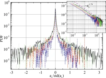
parti-Fig. 4.Probability density function of tracer particle velocity component perpendicular to the mean counterflow, normalized by the standard deviation (see table 2). Figure contains 4 curves, corresponding to 4 heat flux values (or mean counterflow velocities) as in figures 2 to 3, in W/m2: 414 (solid black curve), 590 (dashed red), 608 (dotted green) and 691 (dot-dashed blue). The inset shows the
same data in log-log scale, highlighting the power-law tails with fitted exponent -4.3. The exponent of the power law tail is−4.3±0.3. Temperature is 1.75 K.
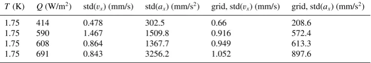
Table 2.Standard deviations for the curves in figures 4 – 7. Meaning of columns:T, temperature;Q, heat flux; std(vx), standard deviation
of tracer particles’ velocity component (figure 4); std(ax), tracer particles’ acceleration (figure 5); grid, std(vx), fluid particles’ velocity
(figure 6) and grid, std(ax), fluid particles’ acceleration (figure 7).
T(K) Q(W/m2) std(v
x) (mm/s) std(ax) (mm/s2) grid, std(vx) (mm/s) grid, std(ax) (mm/s2)
1.75 414 0.478 302.5 0.66 208.6
1.75 590 1.467 1509.8 0.916 572.4
1.75 608 0.864 1367.7 0.949 613.3
1.75 691 0.843 3256.2 1.052 897.6
Table 3.Standard deviations for the curves in figure 8.
grid 1000×1000 600×600 350×350 250×250 90×90 17×17
std(vx) (mm/s) 1.28 1.02 0.894 0.843 0.705 0.496
Fig. 9.Decay of the number of vortex points,N, starting from three initial numbers of vorticesN0: 8192, 4096 and 2048. The
curves corresponding toN0 of 4096 and 2048 are the result of
ensemble averaging of 10 individual calculations. The scaling of the dimensionless time with respect to the real time is the same for all curves and time or axes of the curves are not manipulated in any way: curves naturally collapse onto each other.
cles are found to have power-law tails. The power-law ex-ponent of the fluid particle velocity is consistent with the expected value of−3. Fluid particles and tracer particles have different exponents.
Finally, we found that the decay of the number of vor-tex points obey Vinen’s prediction, indicating that the move-ment of vortex points is random.
6 Acknowledgments
EV and LS acknowledge financial support from the Charles University in Prague under GAUK 366213. CFB acknowl-edges support from the EPSRC.
References
1. K.W. Schwarz, Phys. Rev. B18, (1978) 245-262 2. L. Galantucci,et al.J. Low Temp. Phys. 162 (2011),
354-360
3. W. F. Vinen, Proc. R. Soc. Lond. A242, (1957) 493-515 4. D. R. Tilley and J. Tilley,Superfluidity and
Supercon-ductivity(Hilger, 1990)
5. D. R. Poole,et al., Phys. Rev. B71, (2005) 064514
6. M. La Mantia,et al., J. Fluid. Mech.717(2013) R9 7. A.C. Whiteet al., Phys. Rev. Lett.104, (2010) 075301 8. D. Kivotides, C.F. Barenghi and Y.A. Sergeev, Phys.
Rev. B77, (2008) 014527
9. G. Bewleyet al., PNAS105(2008), 13707-13710 10. S. Zuccheret al., Phys. Fluids24, (2012), 125108 11. R.J. Donnelly and C.F. Barenghi, J. Phys. Chem. Ref.
Data27, (1998) 1217