Best-estimate T/H Uncertainty Analysis using an Optimized Regression Algorithm ACE

(1)

20th International Conference on Structural Mechanics in Reactor Technology (SMiRT 20) Espoo, Finland, August 9-14, 2009 SMiRT 20-Division 3, Paper 2545

A Statistical Uncertainty Assessment on a LOFT L2-5 LBLOCA PCT

Based on ACE-RSM

Kwang-Il Ahn

a

, Bub-Dong Chung

b

, John C. Lee

c

a

Integrated Safety Assessment, KAERI, Daejeon, Korea, [email protected]

b

Thermal-Hydraulic Safety Research Division, KAERI, Daejeon, Korea

c

Dept. of Nuclear Engineering & Radiological Science, Univ. of Michigan, Ann Arbor, MI, USA

Keywords: LBLOCA, PCT, Uncertainty Analysis, Optimal Algorithm, ACE-RSM.

1 ABSTRACT

When a long run time is taken to obtain the relevant output values in a complex physical model (or code), the number of statistical samples which must be evaluated through it is a critical factor in a sampling-based uncertainty analysis. Two alternative methods have been utilized to avoid the problem associated with the size of these statistical samples: one is based on Wilks’ formula and the other is based on the conventional nonlinear regression approach. While both approaches provide a useful means to draw a conclusion on the resultant uncertainty with a limited number of code runs, there are also the corresponding unique limitations. For example, a conclusion based on the Wilks’ formula is highly affected by the sampled values themselves and the conventional regression approach requires a priori estimate on functional forms of a regression model. Main objective of this paper is to introduce a complementary method (based on the ACE algorithm) to the Wilks’ formula and the conventional regression approach for uncertainty analysis and to provide an example application to the OECD BEMUSE Phase III LOFT L2-5 LBLOCA uncertainty analysis.

2 INTRODUCTION

All participants of the OECD BEMUSE Phase-III program [Crecy et al., 2007] utilize the increased number of samples in their uncertainty quantification on the LOFT L2-5 LBLOCA than one required in the first order of Wilks’ formula (i.e., 59) [Wilks, 1941; Nutt et al., 2004] . This was mainly due to one of the observations at the end of BEMUSE-II that the number of code runs should be increased instead of 59 runs that were utilized as a reference case to reduce the dispersion of the uncertainty. Like this, a concern often expressed about a sampling-based uncertainty analysis is to determine the number of samples so that model evaluations will make the cost of the analysis prohibitive. If a statistical meaning could be obtained from the results or an effective uncertainty analysis is possible from them, it is better to reduce a large sample size analysis from the aspect of cost.

From the point of view, the response surface model (RSM) [Sacks et al., 1989] has been used to give an appropriate surrogate model to an original model, by using some use of statistical designs (or a limited number of statistical samples) over all possible ranges of inputs, regression techniques, and optimization methods. This approach is very useful when it takes a long time for code run to obtain the relevant output values (such as a physical trend of performance parameter in a complex physical model) and thus the number of evaluations through it is limited to at most several tens or hundreds. The resultant model is a simple and high speed alternative model that can describe best the trend of the relevant output variable with the specified inputs. Since the functional form of the RSM is generally not known for many cases, it requires a tedious and time-consuming process to obtain the most relevant functional form between input and output parameters (coupled with multivariate nonlinear regression analysis).

(2)

dependent variables while it does not require a priori estimate of the functional forms of transformed variables. Once the optimal transformations are obtained, a simple regression analysis can be performed to determine the functional forms for the transformed dependent and independent variables. Thus, the ACE method offers two distinctive advantages over the traditional nonlinear regression analysis. First, while nonlinear regression analysis requires a priori estimate of functional forms and in general sufficiently accurate estimates of the fitting coefficients to arrive at a converged solution, the ACE algorithm guarantees the convergence of the transformations, and, once the ACE iteration is converged, a simple regression analysis usually suffices to generate actual analytical functional forms for the transformed variables. Second, the ACE algorithm cannot produce a worse fit than the traditional RSM, because if no transformations are found to be necessary, then ACE would simply suggest nearly linear transformations for all the variables, indicating at least equal or much greater data fitting than the traditional RSM. Even though those advantages of the ACE algorithm, its practical use has been very limited in the field of thermal-hydraulic uncertainty analysis [Glaeser, 2000, IAEA, 2008].

Main objective of this paper is to introduce a complementary method (based on the ACE algorithm) to the Wilks’ formula and the conventional regression approach for uncertainty analysis and to provide an example application as a complementary work to the OECD BEMUSE Phase III LOFT L2-5 LBLOCA uncertainty analysis.

3 BRIEF SUMMARY OF THE ACE ALGORITHM

For a dependent variableY and multiple independent variables(X_i,i=1,...,p),the objective of the ACE algorithm [Cleveland, 1979; Breiman et al., 1985; Wang et al., 2005] is to find optimal transformations!(Y)and !_i(X_i)that maximize the statistical correlation between!(Y)and_!_ip"_i(X_i), by treating each value of the transformed variable !(Y)as the expectation of several realizations of the sum of transformed independent variables_!_ip"_i(X_i). The resulting ACE regression model can be expressed as:

! "

#

$(Y)= +_%ip₌1 i(Xi)+ (1)

Thus, the ACE model replaces the problem of estimating a linear function of a p-dimensional variable X=(Xi,X2,...,Xp)by estimating p separate one-dimensional functions, !i(Xi), and !(Y)using an iterative

method. These transformations are achieved by minimizing the unexplained variance of a linear relationship between the transformed response variable !(Y)and the sum of transformed independent variables_!_ip"i(Xi).

The error variance !2that is not explained by the regression (under the constraint,E[!2(Y)]=1)

2 1

2 1 2

] ) ( )

( [ ) ,..., , ,

($ # # #p =E$ Y "_!ip₌#i Xi

% (2)

The minimization of _!2_{with respect to} ₍ _), ₍ _),..., ₍ ₎ 2

2 1

1 X ! X !p Xp

! and !(Y)is carried out through a series

of single-function minimization, involving the following conditional expectation and minimization

2

] | ) ( )

( [ )

( i = #_!pj_"i j j i

i X E% Y $ X X

$ (3a)

|| ] | ) ( [ ||

] | ) ( [ ) (

1 1

!

= =

= _p

i i i

p

i i i

Y X E

Y

" "

# (3b)

On The final !_i(X_i)and !(Y) after the minimization are estimates of the optimal transformations

) (

*

i X

i

! and!*(Y), leading to the following relationship

* 1

* *

) ( )

( " !

# Y =_$ip₌ _i Xi + (4)

(3)

iterative use of the two smoothing operations of Eqs.(3) in alternating directions to obtain transformed independent and dependent variables. When a convergence is attained with an iterative scheme, the data in each transformed variable are usually smooth and slowly varying. Then, selecting simple functional forms for the transformations and performing standard regression analysis for each transformation, we can obtain the final functional form of Y versusX1,...,Xp if ( )

*

Y

! has an inverse function:Y = *"1[_!_ip₌₁ *(X_i)].

i

# $

On the other hand, the error in Eq.(2) could vanish with a judicious choice of!(y), if !(yj)equals )

( i,j i x

! for every point of a set of N data {(xi,j,yj),j=1,2,...,N}. In practice, however, this idealized situation does not occur because the data contain a greater or lesser randomness and so do !(yj)and!i(xi,j). Thus,

) (yj

! is considered, in the ACE algorithm, the expectation of several realizations of!_i(x_i) for the j’th point, rather than a single unique realization !i(xi,j)as in conventional regression analysis. In most regression problems, there is usually only one value yj, and hence one value !i(xi,j), for the j’th data point, and the

conditional expectation !(yj) has to be evaluated with the neighboring values

{

"i(xi,k),k= j!M,...,j+M

}

,

for some M , treated as realizations of !i(xi,j)for the j’th data point. Thus, data smoothing operation over the dependent and independent variables plays a primary role in the ACE algorithm.

4 MARS SIMULATION FOR THE PCT UNCERTAINTY ANALYSIS

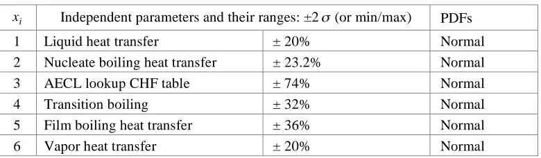
The sampling-based method [Helton et al., 2002] has been required to quantify the overall uncertainty employed in the MARS codes by means of a statistical analysis [Chung, 2005]. In order to assess the PCT uncertainty for a LBLOCA blowdown phase, first, 14 uncertainty parameters have been chosen as a result of Phenomena Identification and Ranking Table (PIRT) on LBLOCA. As given in Table 1, the chosen parameters cover (a) physical models employed in the code and (b) initial and boundary conditions for the LBLOCA simulation. The state of knowledge about all uncertain parameters has been described by ranges and subjective probability distribution (also see Table 1). Second, the random variance of each uncertain parameter was determined by a crude Monte Carlo sampling method according to the combined probability distribution of the uncertain parameters. For uniform distribution, the minimum and maximum values are boundaries of sampling. For normal distribution, the sampling boundaries were truncated at mean ±2! . Any dependency between parameters was not considered in the sampling process. Then, the MARS code calculations have been performed with sampled sets of parameters. In order to limit the number of samples for the MARS code calculations to a reasonable level, a set of 93 samples have been required to apply Wilks’ formula in unilateral at the 2nd order (for 95% tolerance limit and 95% confidence interval of the code results), but 100 samples were sampled to get sufficient calculation numbers to cover the unexpected run errors. Finally, multiple input decks (each input deck has 100 samples) have been implemented to identify the effect of different sets of random samples on the PCT value, consequently resulting in several thousands of PCT values for its statistical analysis. The short transient time (i.e., 100 second in case of LOFT L2-5) enabled to perform the multiple sets of these 100 cases.

During the calculation, the ratio of the failed runs (i.e., crash of the simulation code) was 7% (i.e., 7 out of 100 runs were failed). The failure was random and its reasons were not known (maybe due to a combination of physically unreasonable random values). The failed calculations were discarded manually. The remaining outputs are the final result of the propagation of input uncertainties through the specified number of code calculations.

Table 1. MARS input parameters for PCT uncertainty analysis

i

x Independent parameters and their ranges: ±2! (or min/max) PDFs

1 Liquid heat transfer ± 20% Normal

2 Nucleate boiling heat transfer ± 23.2% Normal

3 AECL lookup CHF table ± 74% Normal

4 Transition boiling ± 32% Normal

5 Film boiling heat transfer ± 36% Normal

(4)

7 Peaking factor(Fq) ± 14.96% Normal

8 Cold gap size ± 20.98mm Uniform

9 Gap conductance ± 80% Uniform

10 Fuel conductivity ± 10% Normal

11 Decay heat ± 6.6% Normal

12 Break area ratio 0.7~1.15 Uniform

13 Pump two-phase performance 0.0~1.0 Uniform 14 Downcomer lateral loss coeff. 0.0~1.0 Uniform

5 FORMULATION OF ACE-RSM MODELS AND THEIR RESULTS

Based on the MARS input xi (p=14) and output values for the PCT (y) uncertainty analysis, the

corresponding ACE-RSM models can be formulated through the following procedures:

(Step-1): Derive two types of the ACE-transformed functional forms for independent and dependent

variables with the prepared N sample input and output values:x_i ~!ˆ_i(x_i) andy~!ˆ(y).

(Step-2): Perform a (piece-wise) linear regression between the transformed variables, !ˆ_i(x_i)and!ˆ(y):

). ( ˆ )

(

ˆ 14

1 * 0

*

i p

i i

i x

y

_!

=

= +

=# #"

$ (5)

Here, it should be noted that when a convergence is well attained with an iterative scheme, a regression of the transformed dependent variable on all the transformed covariates results in all parameter coefficients of the independent variables (!_i,i=1,2,...,p) being positive and close to 1 and the error term"₀ !0.

(Step-3): Derive the final functional form between the original input and output variables, x_iandy:

. ) ( ˆ ˆ

ˆ

14

1 * 0

1 *

! " #

$ % &

+

= '=

= (

i p

i i

i x

y + * * ) (6)

Then, 3 typical ACE-RSM models on the PCT have been formulated based on a limited number of sample runs: (a) one from N=124 (Random Set-1): ACE-RSM-Model-1, (b) one from N=124 (Random Set-2): ACE-RSM-Model-2, (c) one from N=300: ACE-RSM-Model-3. N=124 corresponds to the minimum number of samples required to apply the 4th order of Wilks’ formula (for 95% tolerance limit and 95% confidence level of the code results), and N=300 corresponds to twice the minimum number of samples (N=153) required to apply the 4th order.

As a result of the Step-1, the fitted functions between xiand !ˆi(xi) suggested by the ACE plots have

been obtained by applying the piece-wise linear or polynomial format ofx_i. In addition, the fitted functions between y.and !ˆ(y)have been obtained by applying the piece-wise linear or quadratic format of y. As a result of the Step-2, Figures 1-2 show functional relationships between the original output variable (y) and transformed output variable!ˆ(y) for the above 3 cases and between a sum of transformed inputs

!==114 ( )

p

i "i xi and output !ˆ(y),respectively. Table 2 also shows the regression coefficients (!i,i=1,2,...,p)

between !ˆi(xi)and!ˆ(y). As a result of the Step-3, Figures 3-4 show one-to-one comparison of the

(5)

y-Theta(y) relation

Theta(y) = 1.194E-05y2_{- 1.378E-02y + 1.22} R2_{= 0.9999}

-3 -2 -1 0 1 2 3

700 800 900 1000 1100 1200 1300

y T h e t a ( y ) y-Theta(y) relation

Theta(y) = 9.168E-06y2_{-9.399E-03y - 0.251, R}2_{= 0.98}

-3 -2 -1 0 1 2 3 4

600 700 800 900 1000 1100 1200 1300 1400

y T h e t a ( y ) y-Theta(y) relation

Theta(y) = 9.168E-06y2_{-9.399E-03y - 0.251, R}2_{= 0.98}

-3 -2 -1 0 1 2 3 4

600 700 800 900 1000 1100 1200 1300 1400

y T h e t a ( y )

(a) ACE-RSM-1 (b) ACE-RSM-2 (c) ACE-RSM-3 Figure 1. Functional forms of the ACE-transformed output variable !ˆ(y)

Difference between Sum:Phi(xi) and Theta(y)

y = 1.0056x - 2E-06 R2 = 0.9561

-5 -4 -3 -2 -1 0 1 2 3 4 5

-4 -3 -2 -1 0 1 2 3 4

x=Sum:Phi(xi) y = T h e ta (y )

Difference between Sum:Phi(xi) and Theta(y) y = 1.0074x - 7E-07, R2 = 0.9603

-4 -3 -2 -1 0 1 2 3 4

x=Sum:Phi(xi) y = T h e t a ( y )

Difference between Sum:Phi(x) and Theta(y)

y = 1.0136x - 2E-06 R2 = 0.9256

-4 -3 -2 -1 0 1 2 3 4 5

-4 -3 -2 -1 0 1 2 3 4

x=Sum:Phi(xi)

y=Theta(y)

(a) ACE-RSM-1 (b) ACE-RSM-2 (c) ACE-RSM-3

(a)%ˆ*(y)=1.0056_#ip₌=₁14$ˆi*(xi)!2.0"10!6,

2

R =0.96

(b)%ˆ*(y)=1.0074_#ip₌=₁14$ˆi*(xi)!7.0"10!7,

2

R =0.96

(c)%ˆ*(y)=1.0136_#ip₌=₁14$ˆi*(xi)!2.0"10!6,

2

R =0.93

Figure 2. Relationships between the ACE-transformed inputs !ˆ_i(x_i)(p=14) and output !ˆ(y)

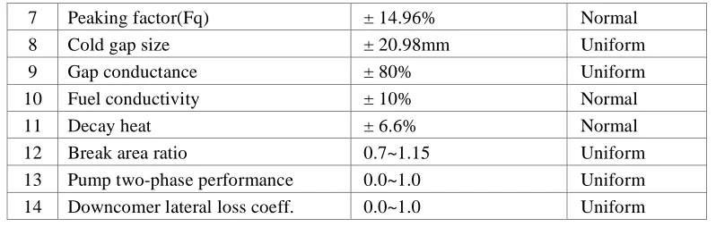
Table 2. Regression coefficients between the ACE-transformed inputs and output.

Regression coeff.(!_i)and the square of the multiple correlation coefficient(R2)

) ( ˆ* i x !

ACE-RSM-1 ACE-RSM-2 ACE-RSM-3

i=0 _!₀= -6.93E-07 !0= -6.93E-07 !0= -2.03E-06

i=1 _!₁= 1.17 !1= 1.67 !1= 1.05

i=2 _!₂= 1.08 !₂= 1.39 !₂= 1.50

i=3 _!₃= 1.27 !3= 1.17 !3= 1.14

i=4 _!₄= 1.08 !4= 0.909 !4= 1.01

i=5 _!₅= 1.18 !5= 1.04 !5= 0.987

i=6 _!₆= 1.21 !₆= 1.48 !₆= 1.17

i=7 _!₇= 1.00 !7= 1.02 !7= 1.01

i=8 _!₈= 1.01 !8= 0.979 !8= 0.993

i=9 _!₉= 0.979 !9= 0.970 !9= 0.985

i=10 _!₁₀= 1.06 !₁₀= 1.10 !₁₀= 1.14

i=11 _!₁₁= 1.14 !11= 0.956 !11= 1.15

i=12 _!₁₂= 1.01 !12= 1.00 !12= 1.01

(6)

i=14 _!₁₄= 0.992 !14= 1.21 !14= 1.10

2

R 0.96 0.96 0.93

The three plots of transformed variables !ˆ*(y)and !ˆ_i*(x_i)in Figure 2 show approximate linearity with higherR , 2 explaining quite good approximations to !*(y)and !i*(xi) with the ACE algorithm. This results are also justified by the regression coefficients (!_i,i=1,2,...,p ) between !ˆ_i(x_i)and !ˆ(y)in Table 3, approaching 1 for most!ˆ*(x_i).

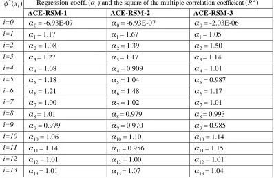
On the other hand, the comparison with the original MARS results (Figures 3-4) explains that except for the lower PCT values (subject to highly nonlinear thermal-hydraulic behavior), the ACE-RSM Models relatively well trace the original MARS results, compared to the corresponding linear regression models (see Table 3). From the qualitative aspect, the ACE-RSM-Model-3 (based on a larger number of samples) is quickly converged to the original results, compared with ACE-RSM-Model-1 and Model-2 subject to higher values ofR2. This fact indicates that although the RSM itself is well fitted to the original code results smaller number of samples may not trace the whole trend of the original MARS code results that are not explained due to their random variation. In order to cover such a random variation that may be not explained by the limited number of samples, it is better to employ appropriate number of samples. From the quantitative aspect, the accuracy bound for ACE- Model-3 is in between !T|MARS-ACE|=5K for 95% PCT and 20K for 5% PCT (e.g., see the case of N=3000 of Table 4). The above results indicate that the ACE-RSM models could give an appropriate surrogate model to the original MARS code, although they also show a greater or less dependency on the utilized number of samples as in the conventional RSM.

N=124 (Random Set1) RMS error= 26.7, NRMS=0.037 (3.7%)

y = 0.9686x + 33.674, R2 = 0.926

700 800 900 1000 1100 1200 1300 1400

x=PCT1(raw)

y=

PC

T1

(a

ce

)

y = 0.923x + 81.411, R2 = 0.9257

500 600 700 800 900 1000 1100 1200 1300 1400 1500

500 700 900 1100 1300 1500 x=PCT1(raw)

y=

PC

T1

(a

ce

)

(a) ACE-Model-1: (b) ACE-Model-2: 2

R =0.9260, Normalized RMS=0.037 (3.7%) R2=0.9257,Normalized RMS=0.044 (4.4%)

Figure 3. Comparison with MARS result (ACE-RSM-1 and 2)

y = 0.9123x + 97.904, R2 = 0.8612

500 600 700 800 900 1000 1100 1200 1300 1400 1500

500 700 900 1100 1300 1500

x=PCT1(raw)

y=

PC

T1

(a

ce

)

ACE-RSM-3: R2=0.8575, Normalized RMS=0.056 (5.6%) Figure 4. Comparison with MARS result (ACE-RSM-3)

(7)

Linear regression between original inputs and output i p

i ix

y

_!

=

= +

= 14

1 0 ˆ " "

Coeff. of determination

! !

= = " "

= N

j j N

j

j y y y

y R

1 2 1

2 2

) ( / ) ˆ (

1st order RSM

Rank regression

Partial correlation

Standardized rank regression

Partial rank correlation

2

R (RSM-1) 0.85 0.85 0.85 0.81 0.81

2

R (RSM-2) 0.84 0.84 0.84 0.82 0.82

2

R (RSM-3) 0.81 0.81 0.81 0.79 0.79

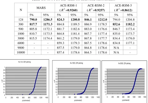
Table 4. 5/95% PCT (K) values for three ACE-RSM models.

MARS ACE-RSM-1

(R2=0.9260)

ACE-RSM-2 (R2=0.9257)

ACE-RSM-3 (R2=0.8612) N

5% 95% 5% 95% 5% 95% 5% 95%

124 790.0 1286.5 824.3 1200.8 846.1 1212.0 794.0 1204.8 300 817.7 1171.3 884.8 1189.5 886.9 1178.5 852.6 1182.2 500 805.8 1172.1 881.7 1182.6 883.0 1176.6 846.7 1173.4 1000 810.7 1173.5 864.8 1181.4 867.7 1177.4 835.0 1173.7 3000 815.5 1174.4 861.2 1179.0 867.8 1177.7 834.4 1176.0 6000 - - 859.3 1179.3 867.5 1178.6 834.8 1177.1

9000 - - 857.5 1179.0 864.8 1178.6 N/A -

10000 - - 857.4 1178.6 864.5 1178.6 N/A -

N=124, CDF plotting

0 0.1 0.2 0.3 0.4 0.5 0.6 0.7 0.8 0.9 1

0 200 400 600 800 1000 1200 1400 y(estimated)

c

d

f

N=1000, CDF plotting

0 0.1 0.2 0.3 0.4 0.5 0.6 0.7 0.8 0.9 1

0 200 400 600 800 1000 1200 1400 y(estimated)

c

d

f

N=3000, CDF plotting

0 0.1 0.2 0.3 0.4 0.5 0.6 0.7 0.8 0.91

0 200 400 600 800 1000 1200 1400 y(estimated)

c

d

f

Figure 5. CDF variation according to the increase of sample N (based on ACE-RSM-1)

6 CONCLUSION

The ACE-RSM approach has been applied to assess the blowdown PCT uncertainty for the LOFT L2-5 Experiment as a complementary work to the OECD BEMUSE Phase-III program. A comparison with the original code results shows that except for the lower PCT values (subject to highly nonlinear thermal-hydraulic behaviour), the formulated ACE-RSM Models relatively well trace the original code results, even with a limited number of code runs. Since the aforementioned nonlinear thermal-hydraulic behaviour highly depends on a physical domain of a system rather than a random error, its impact on the final results should be explained by the other means in more detail (e.g., physical models employed in the thermal-hydraulic system code).

(8)

Acknowledgements. This work was supported by Nuclear Research & Development Program of the Korea

Science and Engineering Foundation (KOSEF) grant funded by the Korean government (MEST).

REFERENCES

Breiman L., and Friedman, J.H. 1985. Estimating optimal transformations for multiple regression and correlation, Journal of American Statistical Association, Vol. 80, p.580-598.

Chung, B. D. 2005. Uncertainty quantification of LOFT L2-5 experiment, presented in OECD/NEA BEMUSE phase III activity 3rd meeting, October 26-28, Grenoble, France.

Cleveland, W. S. 1979. Robust locally weighted regression and smoothing scatterplots, Journal of American Statistical Association,Vol. 74, p.828-836.

Crécy, A., and Bazin, P. 2007. BEMUSE phase III report: uncertainty and sensitivity analysis of the LOFT L2-5 test, CEA, France.

Glaeser, H. 2000. Uncertainty evaluation of thermal-hydraulic code results, International Meeting on "Best-Estimate" Methods in Nuclear Installation Safety Analysis (BE-2000), Washington, DC, November.

Helton, J. C. and Davis, F. J. 2002. Illustration of Sampling-Based Methods for Uncertainty and Sensitivity Analysis, Risk Analysis, Vol. 22: 3, p.591-622.

Iman, R. L., and Shortencarier, M. J. 1984. A fortran 77 program and user’s guide for the generation of Latin Hypercube and Random Samples for use with computer models, NUREG/CR-3624, Technical Report SAND83-2365, Sandia National Laboratories, Albuquerque, NM.

IAEA, 2008. Best estimate safety analysis for nuclear power plants: uncertainty evaluation, IAEA Safety Reports Series No.52, Vienna, Austria.

Nutt, W. T. and Wallis, G. B. 2004. Evaluation of nuclear safety from the outputs of computer codes, Reliability Engineering and System Safety, Vol.83, p.57–77.

Wang, D. and Murphy, M. 2005. Identifying Nonlinear Relationships in Regression using the ACE Algorithm, Journal of Applied Statistics, Vol. 32:3, p.243–258.

McKay, M. D., Bechman, R. J., and Conover, W. J. 1979. A comparison of three methods for selecting values of input variables in the analysis of output from a computer code, Technimetrics, Vol. 21:2, p.239– 245.

Sacks, J., Welch, W. J., Mitchell, T. J., and Wynn, H. P. 1989. Design and analysis of computer experiments,

Statistical Science, Vol. 4:4, p. 409–435.