ABSTRACT
ZHOU, JINGWEN. Calibration of Numerical Model Output Using Nonparametric Spatial Density Functions. (Under the direction of Montserrat Fuentes.)
Studies on the health impacts of climate change routinely use climate model output as future
exposure. However, climate model simulations are deterministic, thus resolving the differences
between climate model output and the observed data in terms of their entire distributions
is of critical interest for air quality management. For health impact analysis, uncertainty
quantification is an important component of the risk assessment process and has been limited
to the variability due to different emission scenarios or multi-model ensembles in the form
of sensitivity analysis. While the uncertainty associated with climate model output is well
recognized, it is difficult to assess its magnitude for any single climate model.
Spatial quantile calibration approach is motivated by the need to better characterize the
tails of future exposure distributions where the greatest health impacts are likely to occur.
Specifically, quantile calibration seeks to model a monotonic transformation function from the
entire quantile process of the model output distribution to the quantile process of the observed
data distribution jointly. To this end, we use a Bayesian framework to model the quantile
processes. The corresponding likelihood approximation is innovatively derived by a mixture
density where the central tendency is given by the estimated quantile functions and the tails
follow a generalized Pareto distribution. In addition, spatial techniques have been developed
to incorporate spatial dependence into the model, which allows us to downscale the gridded
climate model output to point-level for projecting exposure over a specific geographical region.
By modeling climate model output to reproduce small-scale weather events in a historical period
where observations are available, this dissertation not only calibrates future model projections
that incorporate a spatial adjustment of the entire distribution of the model output with respect
to the distribution of the monitoring data, but also accounts for projection uncertainty in the
In each chapter, we present an application for the introduced method. Our approach is able
to achieve reduction in the root mean square error (RMSE) compared to the default approach
based on the first two moments of the climate model output and the observed data.
In Chapter 1, we motivate this work by introducing and demonstrating the utility of both
quantile calibration and spatial adjustment separately.
In Chapter 2, we present the spatial quantile process. We apply a nonlinear monotonic
regression approach to the quantile functions taking into account the spatial dependence. We
investigates the properties of this spatial quantile process, and present a simulation example to
illustrate the utility of this model.
In Chapter 3, we extend the single spatial quantile process to construct the calibration
function which maps the climate model quantile process to the quantile functions estimated
from the observed data. Subsequently, a spatial adjustment of the entire distribution of the
model output with respect to the distribution of the monitoring data was specified to downscale
the calibration function and their spatial-quantile processes. As an example, we apply this
calibration approach to real ozone data.
In Chapter 4, we outline the modeling steps for risk estimation and how to utilize calibrated
model projections to conduct health impact analyses associated with extreme weather
condi-tions. As an example, we apply the methodology to calibrate temperature projections from a
regional climate model for the period 2041 to 2050. Accounting for calibration uncertainty, we
calculated the number of of excess deaths attributed to future temperature for three cities in
c
Copyright 2012 by Jingwen Zhou
Calibration of Numerical Model Output Using Nonparametric Spatial Density Functions
by Jingwen Zhou
A dissertation submitted to the Graduate Faculty of North Carolina State University
in partial fulfillment of the requirements for the Degree of
Doctor of Philosophy
Statistics
Raleigh, North Carolina
2012
APPROVED BY:
Sujit Ghosh Brian Reich
Jerry Davis Frederick Bingham
DEDICATION
This thesis is dedicated to my parents who have supported me all the way since the beginning
BIOGRAPHY
I was born in Xian, China and studied mathematics and applied mathematics at the University
of Science and Technology of Beijing (USTB) in 2000. Following my undergraduate studies,
I received a M.S. in statistics from University of Science and Technology of China (USTC),
specializing in Bayesian statistics. In year 2007, I entered the Department of Statistics at the
North Carolina State University (NCSU).
While at the NCSU, I was taught Experimental Design, Data Mining and Machine Learning,
Measure Theory, Advanced Inference, Time Series, Spatial Statistics and Bayesian Statistics.
These theoretical classes helped me obtain a deeper understanding of statistical methods
de-velopment.
In 2009, I was supported as a research assistant, working in support of ongoing research
projects regarding the environment science, especially in aspects of field (model output) data
collection and analysis. Based on an application for describing the impact of climate change
on the public health, I was interested in methods for calibrating the model output when the
observations are not available, which turned out to be the topic of my doctoral thesis. I also
frequently used geostatistical tools in my work: mapping pollutants distributions, analyzing
spatial relationships, and examining spatial-quantile changes over time. I spent three years and
ACKNOWLEDGEMENTS
It would not have been possible to write this doctoral thesis without the help and support of
the kind people around me, to only some of whom it is possible to give particular mention here.
Above all, I would like to thank my principal supervisor Prof. Fuentes for her help, support
and patience, not to mention her advice and unsurpassed knowledge of statistics. The good
advice, support and friendship of my second supervisor, Dr. Davis, has been invaluable on both
an academic and a personal level, for which I am very grateful. I would like to acknowledge
the financial, academic and technical support of the Department of statistics and its staff,
particularly in the award that provided the necessary financial support for this research. The
library facilities and computer facilities of the University have been indispensable.
I am most grateful to Dr. Reich for providing me with computer files of his work, which
have been a valuable and reliable method of checking the published editions and have made
referencing quotations from the texts far more efficient. I would like to thank Alison for her
kindness, friendship and support. I remember the generosity and encouragement of Dr.
Ar-roway, when I first became interested in NCSU. All her efforts in promoting a stimulating and
welcoming academic and social environment will stand as an example to those that succeed
them.
I would like to thank my friends Hans Huang for his personal support and great patience
at all times. My parents have given me their unequivocal support throughout, as always, for
which my mere expression of thanks likewise does not suffice. Last, but by no means least, I
would also like to thank my colleagues and friends Brenda, Lan, Lixia and elsewhere for their
support and encouragement throughout.
For any errors or inadequacies that may remain in this work, of course, the responsibility
TABLE OF CONTENTS
List of Tables . . . vii
List of Figures . . . .viii
Chapter 1 Introduction . . . 1
1.1 Motivation . . . 3
1.2 Literature review . . . 6
1.2.1 Quantile functions and density quantile approach . . . 6
1.2.2 Frequentist method for quantile regression . . . 9
1.2.3 Bayesian method for quantile regression . . . 11
1.3 Spatial models . . . 12
1.4 Notation . . . 13
1.5 Outline . . . 14
Chapter 2 Spatial quantile process . . . 16
2.1 Spatial quantile regression . . . 16
2.1.1 Spatial-quantile function . . . 16
2.1.2 Estimation . . . 19
2.2 Spatial-temporal quantile regression . . . 22
2.3 Simulation study . . . 22
2.4 Summary . . . 23
Chapter 3 Spatial quantile calibration . . . 26
3.1 Spatial quantile calibration of deterministic model output . . . 26
3.2 Spatial-temporal quantile calibration . . . 28
3.3 Estimation . . . 29
3.4 Application: calibration of eastern US ozone data . . . 32
3.4.1 Data description . . . 32
3.4.2 Result analysis and discussion . . . 33
Chapter 4 Mortality prediction with calibrated meteorological variables . . . . 42
4.1 System calibration and spatial quantile processes . . . 43
4.2 Health Effect Estimation and Impact Analysis . . . 46
4.3 Estimation . . . 48
4.4 Case study of the heat wave . . . 49
4.4.1 Data description . . . 49
4.4.2 Result analysis . . . 50
4.5 Summary . . . 53
Chapter 5 Discussion and Future work . . . 63
Appendix . . . 70
Appendix A Appendix . . . 71
A.1 Proper posterior distribution . . . 71
LIST OF TABLES
Table 2.1 (Example 2) Empirical root mean integrated squared error (×100), with its standard error in parentheses . . . 23
Table 4.1 Posterior medians (95% credible intervals) of the annual excess deaths attributable to high temperature and heat waves across three Alabama cities. For high temperature, the baseline group is defined as days with maximum temperature under 30◦C and the at-risk group is defined as days with maximum temperature above the threshold. For heat wave, the at-risk group is defined as days with maximum temperature above the quantile threshold. . . 61 Table 4.2 Observed and projected average number of high temperature days and
LIST OF FIGURES
Figure 1.1 The linear regression (LM) predictor for CMAQ at a selected monitoring site. The left panel shows the corresponding 100τthquantile curves of the monitoring
data and linear-transformed model output, units in parts per billion (ppb); while the right panel is the corresponding quantile-quantile plot. . . 5 Figure 1.2 Calibration functionGτ with respect to the underlying quantile processes. . . . 8 Figure 1.3 Quantile regression splines can cross each other, so it does not provide a
valid quantile function. . . 10
Figure 2.1 The comparison between the I-splines of orderh=3 and the integrated Bernstein polynomials of degree 4. The I-splines are defined on [0, 1] and are associated with interior knots 0.2, 0.8. Each I-spline is piecewise cubic, and a monotonic curve is obtained by the linear combination of these M=5 splines with non-negative coefficients. The I-spline function is used to ensure the non-crossing quantiles with both flexibility and constrains at different percentiles. . . 17 Figure 2.2 The probability density function for the generalized Pareto distribution is
plot-ted with respect to the different tail index parametersκ. The parameter ranges
κ >0,κ= 0, andκ <0 correspond to the short tails, exponential type and long tails, respectively. . . 21 Figure 2.3 Bayesian nonparametric quantile (BSQ) regression from Example 2. Interior
knots are placed at 0.2, 0.8 withδ= 0.005 andκ= 0. We add a sin function to mimic the temporal trend in reality. We obtain the conditional quantile estimates for τ= 0.01, 0.5, 0.9 and 0.99. Notice that the classic quantile regression spline generates crossing quantile curves, which does not provide a valid quantile process. 25
Figure 3.1 A process chart for spatial quantile calibration for going from model output to the observations. We calibrate the original model output with the corresponding observations through their underlying spatial-quantile processes. Both of the model output quantile modeling and the adjustment of the entire distribution of model output with respect to the distribution of monitoring data need to be across space. . . 36 Figure 3.2 Maps of the sample 90thquantile levels of the ozone concentrations for both the
CMAQ output and observations; At a randomly selected site (i.e., 59th) where we
have T=153 observations; we use ”∗” to represent its location. The histogram, sample quantile and density function of the two data sources are provided to identify the different behave in their distribution. . . 37 Figure 3.3 Quantile comparison plots. Maps of the 5th, 50th and 95th quantiles for the
Figure 3.4 The Bayesian spatial-quantile calibration for CMAQ at a selected monitoring site. The left panel shows the corresponding 100τthquantile curves of the
mon-itoring data andGτ-transformed model output, units in parts per billion (ppb);
while the right panel is the corresponding quantile-quantile plot. . . 39 Figure 3.5 The scale predictor for CMAQ at a selected monitoring site. The left panel
shows the corresponding 100τthquantile curves of the monitoring data and scale-transformed model output, units in parts per billion (ppb); while the right panel is the corresponding quantile-quantile plot. . . 40 Figure 3.6 The 95thquantile for the monitoring data (units in ppb), using both the quantile
calibration and linear regression method. We compare the differences between the linear regression and the Bayesian quantile calibration methods in terms of theRM SE. . . 41
Figure 4.1 A process chart for our two-stage estimation. We first obtained the calibration model by comparing the original NARCCAP data with the corresponding ob-servations through their underlying spatial-quantile processes in year 2000. We then fitted the health model to investigate the relationship between heat waves and mortality. Finally, we evaluated the future heat wave excess mortality based on the calibrated NARCCAP maximum temperature from 2041 to 2050. . . 55 Figure 4.2 Likelihood estimation without specifying a density function a priori. The blue
curve is a density plot of simulated data. The likelihood function expressed as a quantile-based central tendency and a generalized Pareto tail are able to characterize the unbounded response variables. . . 56 Figure 4.3 Quantile-quantile plot of the model output and the observations. The blue
curve is an estimatedGτ function. . . 57 Figure 4.4 Locations of the monitoring sites (blue triangles), centers of the NARCCAP
grid cells (red dots) and NMMAPS communities (green circles) within Alabama. 58 Figure 4.5 At three urban communities Birmingham (birm), Mobile (Mobi), and Huntsville
(hunt), we plot τth quantile curves of NARCCAP outputs, observations, our Bayeisan calibrations and the simple linear regression (LM) of daily maximum temperature in year 2000, units in Celsius (C).. . . 59 Figure 4.6 τthquantile curves of the historical NARCCAP data, the corresponding
obser-vations, the uncalibrated future model output and the calibrated daily maximum temperature, unit in Celsius. Note that the discrepancies mostly occurred at the lower tail of the distribution. . . 60
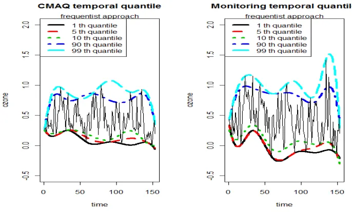
Figure 5.1 The CMAQ and monitoring temporal quantiles at site 4. Under the non-crossing constraints, ozone quantile curves show little trend for both the CMAQ models and the monitoring data. . . 65 Figure 5.2 Temporal quantile surfaces on site 19 for both the CMAQ data and Observed
Chapter 1
Introduction
Climate change poses unique challenges to human health. Unlike health threats caused by a
particular disease, climate change can lead to potentially harmful health effects. For instance,
there are direct health impacts from heat waves, ailments caused by air pollutants such as ozone
and many climate-sensitive infectious diseases. The assessment of potential health effects of
cli-mate change must include consideration of the capacity to manage new and changing clicli-mate
conditions.
Projections from climate models provide state-of-the-art quantitative information on future
climate. Recently, climate model output has been utilized to quantify the health impacts of
var-ious environmental risk factors due to climate change. Using a large number of grid cells, they
generate averaged concentrations which have full spatial coverage and high temporal resolution
without missing values. However climate model simulations are deterministic, and uncertainty
may be present in various modeling stages that attempt to represent the underlying physical
processes with numerical models [Knutti, 2008]. Uncertainties about the model outputs should
be recognized [Kennedy and O’Hagan, 2001; Paciorek, 2011]. The various sources of such
uncer-tainties are classified as low quality of emissions data, model inadequacy and residual variability
the other hand, health impact analysis has focused predominantly on the variability that arise
from different emission scenarios or multi-model ensembles [Peng et al., 2011]. Nevertheless,
the quantification of uncertainty caused by deterministic model output has not been extensively
studied.
In this thesis, we do not calibrate the computer model parameters, for instance, as in
Kennedy and O’Hagan [2001]. Instead we focus on comparing, evaluating and resolving the
differences in the distribution between the model outputs and the observed data. We describe
a Bayesian spatial quantile regression model to calibrate climate model output and use daily
maximum temperature as the motivating example. Temperature projections have been used
extensively in health impacts analysis because of its well-established adverse health effects
[Anderson and Bell, 2009; Curriero et al., 2002]. Moreover, temperature can act as a predictor
for other environmental processes such as infectious disease transmission [Ogden et al., 2006;
Remais et al., 2008], hydrological dynamics for water quality [John and Rose, 2005], or
ground-level ozone creation [Bell et al., 2007; Knowlton et al., 2004]. By modeling climate model output
to reproduce small-scale weather events in a historical period where observations are available,
we want to not only calibrate future model projections, but also incorporate projection
uncer-tainty in the final health impact estimates.
Early evaluation of model performance usually relies on linear least-squares analysis of
ob-servations versus model outputs. However, the model outputs and the obob-servations are on
different spatial scales; this is referred to as the “change of support” problem. The
measure-ments are made at specific locations in the spatial domain, while modeled concentrations are
recorded as averages over grid cells [Eder and Yu, 2006]. Thus the two data sources are not
directly comparable. In regard to this problem, efforts have been made in the recent
litera-ture to address the spatial “incommensurability” between gridded model averages and point
the model outputs as the integral over a grid cell of a latent point-level process, which is also
related to the observations. Additionally, to achieve computational efficiency, Berrocal et al.
[2010] proposed univariate downscaler using a linear regression model with spatially-varying
coefficients, thus developing a “spatial-temporal” model to adjust for the potential spatial
mis-alignment.
Another challenge arises from the usual Gaussian assumption in the standard linear
regres-sion approach which may underestimate the tail probability for climate variables with skewed
distributions [Chang et al., 2010]. For instance, a local heat wave is often defined based on
daily temperatures exceeding the 95th percentile of its local summer time climatology. Another example is the U.S. EPA ozone standards which rely on the fourth highest day of the year
(99th quantile). Therefore improving the ability to characterize extreme temperature events is of critical importance. As a result, we need a method which allows researchers to adjust for the
spatial dependence of the two data sources, and in some sense, to obtain a complete
transfor-mation between the model output and monitoring data in terms of their entire distribution.
Further developments of these proposed evaluation procedures are needed. In this thesis,
we are concerned with the discrepancy due to the shape of the distributions, especially the
tails. In order to compare the density functions of the numerical models and field data, we
esti-mate the spatial quantile functions for both models and data, and we apply a nonlinear spatial
monotonic regression approach to the quantile functions. We use a Bayesian approach for
es-timating and fitting in order to characterize the uncertainties in the data and statistical models.
1.1
Motivation
To illustrate the necessity of the quantile regression approach, we start by using the standard
Sup-pose we have two data sets Y(t,si) and Z(t,Bsi), where s = (s1, s2) is a point measured by
EPA monitors using the latitude/longitude coordinates and Bs the associated model output
simulated grid cell in which s lies, for time t=1,2,...,T, and location i=1,2,...,ns. Based on
the comparison of means and variances, we define the linear regression (LM) model at a given
locationsi∗ as:
E(Y(t,si∗)|Z(t,Bs
i∗)) =β0i∗+β1i∗Z(t,Bsi∗), (1.1)
In other words, the LM model fits the conditional mean of a vector of field dataY(·,si∗), given
the corresponding model outputsZ(·,Bsi∗). It is known that the solution to the ordinary least
squares regression is an optimization problem as follows:
ˆ
β=argminβ X
t
(Y(t,si∗)−β0i∗−β1i∗Z(t,Bs i∗))
2. (1.2)
In addition, if the normality assumption holds, that is:
Y(·,si∗)|Z(·,Bs
i∗)∼ N(β0i∗+β1i∗Z(·,Bsi∗), σ 2I
T)), (1.3)
Then the LM estimator βˆ is normally distributed and reaches the Cram´er−Rao bound for the model, and thus is optimal in the class of all unbiased estimators. Subsequently, the least
squares (LM) estimates ˆβ0i∗ and ˆβ1i∗ are used to calibrate model output as:
ˆ
y(t,si∗) = ˆβ0i∗+ ˆβ1i∗z(t,Bs
i∗). (1.4)
Although the calibrated series ˆy(t,si∗) provide an unbiased estimates of the field data, the
p-value = 0.00576 of a Two-sample Kolmogorov-Smirnov test indicates that the LM estimator
fails to transform the tails of the model output distribution to the corresponding observed
distribution (see Figure 1.1) and capture the non-linear relationship between the quantiles of
observed distribution and the quantiles of the model output distribution (see the
adequate modeling platform when different parts of the observed distribution are suspected to
transform from the corresponding parts of the model output distribution at different rates.
Figure 1.1: The linear regression (LM) predictor for CMAQ at a selected monitoring site. The left panel shows the corresponding 100τth quantile curves of the monitoring data and linear-transformed model
1.2
Literature review
1.2.1 Quantile functions and density quantile approach
Heavy tail distributions are important in many scientific and economical studies. Their
ap-plications include use in the analysis of the impact of extreme event on air quality, and in
the modeling of large insurance claims, among others. In general, it is hard to choose an
ap-propriate distribution for a specific application a priori. To this end it is useful to determine
probability distributions by their tail behavior. Specifically, the density-quantile functions, introduced by Parzen [1979], was widely used as a measure of tail orderings. Given data
z(1,Bsi∗), z(2,Bsi∗)..., z(T,Bsi∗), we want to find statistical patterns in the data. That is, we
seek to model the distribution functionFZ(z) =P(Z(·,Bsi∗)≤z) and the probability density
fZ(z) = FZ0(z). To develop nonparametric statistical data modeling based on estimating the
quantile functions (inverse CDF), we defineqZ(·,Bsi∗)(τ) as:
qZ(·,Bsi∗)(τ) =F −1
Z (τ) = inf{z:FZ(z)≥τ}. (1.5)
Consequently, Z(·,Bsi∗) is identically distributed as qZ(·,Bsi∗)(U), where U is uniformly
dis-tributed on [0,1], because:
P(qZ(·,Bsi∗)(U)≤z) =P(U ≤FZ(z)) =FZ(z). (1.6)
Such identically distributed properties can be rewritten as:
Z(·,Bsi∗)∼qZ(·,Bsi∗)(U).
Suppose FZ is a continuous distribution function, then FZ(qZ(·,Bsi∗)(τ)) = τ for all τ. Thus,
by taking derivatives, it follows that
fZ(qZ(·,Bsi∗)(τ))q 0
Here fZ(qZ(·,Bsi∗)(τ)) is defined to be the density quantile function and model (1.7) implies:
fZ(qZ(·,Bsi∗)(τ)) =
1 q0Z(·,B
si∗)(τ)
. (1.8)
An examination of the density-quantile functionsfZ(qZ(τ)) of familiar probability laws indicates that they can be classified according to their limiting behavior asτ tends to 0 or 1. The behavior
when τ →1 is described as by Parzen [1979]:
fZ(qZ(·,Bsi∗)(τ))∼(1−τ)
υ, υ >0. (1.9)
Tail behavior is classified as (1) short tails or limited type (υ <1); (2) medium tails or
expo-nential type (υ= 1) ; (3) long tails or Cauchy type (υ >1). Additionally, Tokdar and Kadane
[2011] provide an efficient algorithm to solve τ(z) of the equation z = qZ(·,Bsi∗)(τ) in τ. We
make use of the model output that the density quantile function (1.8) lends itself to a likelihood
function which could be further used in the Bayesian analysis (see Section 2.1.2).
However, researchers specializing in calibration techniques are specifically interested in
in-vestigating the difference across quantiles. Indeed, another important property of quantile
functions is how they behave under transformations of random variables. For instance, in
or-der to take the entire distributions of both model outputs and field data into account, let the
100τth quantile process of the observations be denoted by qY(τ,si∗) and the model output as
qZ(τ,Bsi∗). Similarly, denote the distribution functions ofY andZ byFY andFZ respectively.
Now consider the calibration functionGτ. In fact,Gτ(·) is a monotonic function of the quantile functions of model output. For instance, given the quantile levelτ, we use the quantile functions
qY(·,si∗)(τ) andqZ(·,Bsi∗)(τ) to construct Gτ(·) as follows:
In addition, if FZ is a strictly increasing continuous distribution, then:
qY(τ,si∗) =Gτ(qZ(τ,Bs
i∗)). (1.11)
In general, if the data z(1,Bsi∗), z(2,Bsi∗)..., z(T,Bsi∗) are assumed to be identically
dis-tributed as Z(·,Bsi∗), and if the quantile function of Z can be transformed to the quantile
function of a random variable Y by an increasing continuous transformation Gτ, then the
transformed data Gτ(z(1,Bsi∗)), Gτ(z(2,Bsi∗)),..., Gτ(z(T,Bsi∗)) are identically distributed
asY(·,si∗):
P(Gτ(Z(τ,Bsi∗))≤qY(τ,si∗)) = P(Gτ(Z(τ,Bsi∗))≤Gτ(qZ(τ,Bsi∗)))
= P(Z(τ,Bsi∗)≤qZ(τ,Bsi∗)) =τ (1.12)
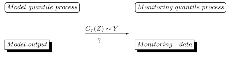
In summary, in order to characterize a transformation from model outputs to the monitoring
data, we are seeking an appropriate function Gτ through their underlying quantile processes
(See Figure 1.2). In addition, examining the changes between the model outputs and monitoring
quantiles can yield a calibration of their overall distributions. This quantile calibration is used
to target a specific part of the distribution of Y, encoded by the corresponding part of the
distribution ofZ. In particular, interest focuses on a suitable framework to study these changes
in the form of quantile processes, where the rate of the change can be different in the tails and
other noncentral or central parts of the distributions.
M odel output M onitoring data
-Gτ(Z)∼Y ?
M odel quantile process M onitoring quantile process
1.2.2 Frequentist method for quantile regression
Quantile regression[Koenker, 2005] is an increasingly popular choice to complement the LM
model. Modeling of the median is a more robust technique than mean regression when dealing
with outlying observations. At each quantile level, we model qZ(t,B
si∗)(τ) (1.5) as:
qZ(·,Bsi∗)(τ) =β1(τ), (1.13)
Where β1(τ) is the coefficient for the τth quantile level. In general, the classical τth sample
quantile estimate is obtained by:
ˆ
β1(τ) = arg min
β1∈R
T
X
t=1
ρτ(z(t,Bsi∗)−β1)
= arg min β1∈R
(τ−1)
X
z(t,Bsi∗)<β1
(z(t,Bsi∗)−β1) +τ
X
z(t,Bsi∗)≥β1
(z(t,Bsi∗)−β1)
Further, let ut = (1, ut2..., utJ) for t= 1, . . . , T, correspond to the J-1 degree spline
repre-sentation of the nonlinear temporal component; we introduce a nonlinear temporal trend in the
quantile process as follows:
qZ(·,Bsi∗)(τ|ut) =u 0
tβ(τ), (1.14)
Given the distribution function of Z(t,Bsi∗), β(τ) can be obtained by solving:
β(τ) = arg min
β∈RJ
E(ρτ(z(t,Bsi∗)−u 0
tβ)), (1.15)
Solving the sample analog gives the estimator ofβ:
ˆ
β(τ) = arg min
β∈RJ
T
X
t=1
(ρτ(z(t,Bsi∗)−u 0
tβ)), (1.16)
However, different quantile levels are analyzed separately. When researchers want to use
Figure 1.3: Quantile regression splines can cross each other, so it does not provide a valid quantile function.
thus it does not provide a valid quantile function. Consider an example of quantile regression
to model the temporal effect on the ozone series in Figure 1.3. The goal is to examine the
8-hour maximum ozone for both model output and monitoring data based on the temporal
components ut. We use these data to fit a quantile regression at the set of percentiles (0.01,
0.05, 0.1, 0.9, 0.99). The fitted curves of the quantile functions give the effects across time.
Conditioning ont= 53, the 90th percentile of the distribution for model output is even higher than the 99th percentile, indicating an invalid quantile function. Also, because little data are obtained at the upper quantiles (extreme event), it is even more problematic to fit individual
quantile curves.
In regard to this problem, He [1997] proposed a location-scale shift method to estimate
the multiple quantile curves while ensuring non-crossing. However, as noted by Bondell et al.
[2010], the response distribution may be affected by the predictors in a less structured manner,
Wu and Liu [2009] proposed a stepwise method by fitting the multiple quantile sequentially
to ensure non-crossing. Although this method provides a flexible model, the algorithm may
depend on the order that the quantiles are fitted. Another computationally efficient approach
is linear programming. Bondell et al. [2010] discussed the performance of adding constrained
estimators to the typical regression quantiles as follows:
ˆ
β(τ) = arg min
β∈RJ
K
X
k=1
T
X
t=1
(ρτk(z(t,Bsi∗)−u 0 tβτk)),
subject to u0tβτk ≥ut0βτk−1, for all k = 2, ..., K (1.17)
Arguably, these multiple quantile fittings in a discrete manner may depend on the number and
location of included quantiles. Tokdar and Kadane [2011] proposed a simultaneous quantile
fit-ting approach to describe the full potential of the model: {qZ(·,B
si∗)(τ|ut) =u 0
tβ(τ); for all 0≤
τ ≤1}.
1.2.3 Bayesian method for quantile regression
In general, quantile functions are useful in determining probability distributions by their tail
behavior, especially for extreme events. To this end we do not choose a distribution for a
spe-cific application a priori, and let the quantile function lead us to a density function. In such a
situation there is uncertainty about the distribution; the Bayesian nonparametric methods are
useful. However, the non-fully specified likelihood makes a posterior density hard to calculate.
To solve this problem, Lavine [1995] introduced a substitution likelihood approach which
depends only on θ, a vector of quantiles of the distribution function FZ. By splitting the
quantile values θ = (−∞ = θ0, θ1, θ2, ..., θK, θK+1 = ∞) into separate bins. Let H(θ) =
which the real line is divided by θ. The substitution likelihood is then defined as:
s(θ) =
T
H1 H2 ... HK+1
Y
∆FZi
Hi, (1.18)
where ∆FZ = (FZ(θ1), FZ(θ2)−FZ(θ1), ...,1−FZ(θK)). In 2005, Dunson and Taylor [2005] applied this approximation approach in a Bayesian framework, where the posterior densities are
determined by a vector of quantiles and truncated priors. However, multiple quantile fittings in
this discrete manner may not satisfy the calibration techniques which are specifically interested
in investigating the difference across quantiles (see Formula (1.11)).
Besides the approximation methods, The quantile regression approach also influenced early
attempts at a Bayesian analysis of (1.14). For the response constructed asz=u0tβ(τ) +,has
the asymmetric Laplace densityf() = const ×exp(−(τ −1I( <0)))[Yu and Moyeed, 2001]. Kozumi and Kobayashi [2011] developed a Gibbs sampling algorithm based on a location-scale
mixture presentation of the asymmetric Laplace distribution from a Bayesian point of view.
Although this approach achieves the computational efficiency, it analyzes different quantile
levels separately.
1.3
Spatial models
In this section we focus on the analysis of spatial models, particularly, using Gaussian processes.
In the case of point-level data, the location indexs(s=1,2,...,ns) varies continuously over a fixed subset of Rd. Based on the normality assumption at one single location in formula (1.3), let
Y(·,s) be a Gaussian process with meanβ0+β1Z(·,Bs) and covariance functionc(s, s0;φ, σ2) =
σ2ρ(s, s0;φ) +τ2I(s=s0) where I denotes the indicator function (i.e.,I(s=s0) = 1 if s=s0
and 0 otherwise). Denote such a Gaussian process by:
Suppose that the covariance between the random variables at two locations depends on their
dis-tance with the exponential association. For insdis-tance, the covariance betweenY(·,s) andY(·,s0) is an exponential function of the interpolation distance; in other words,Cov(Y(·,s), Y(·,s0)) = σ2φ(s, s0;ρ)) +τ2I(s = s0) = σ2exp(−ks−ρs0k) +τ2I(s= s0), where k s−s0 k is the distance between locations s and s0, and σ2 and φ are positive parameters. Also, when s = s0, or ks−s0 k= 0, we haveV ar(Y(·,s)) =σ2+τ2.
An alternative model for the above Gaussian stationary process model (1.19) is:
Y(·,s) =β0(s) +β1(s)Z(·,Bs) +(s), (s)∼N(0, τ2) (1.20)
whereβ0(s) =β0+β0(s) andβ1(s) =β1+β1(s), and(s) is a white noise process with nugget
variance τ2. Then β0(s) and β1(s) can be interpreted as random spatial adjustments at
loca-tion sto the overall additive biasβ0 and the multiplicative bias of model output, respectively.
By modelingβ0(s) andβ1(s) as bivariate zero-mean spatial Gaussian processes using the
core-gionalization approach, Berrocal et al. [2010] introduced a downscaling technique based on the
point-level model for model output, thus obtaining the spatial interpolation at a new location
from the predictive distribution, i.e., sampling f(Y(s0)|Y(·,s), Z(·,Bs)) at location s0. This
downscaling model provides calibration at the local level and allows for a spatial processY(·,s) with a flexible covariance structure. We notice that there is only the normality assumption,
thus it is hard to capture the tail differences when we have the skew distributions.
1.4
Notation
In this section, we introduce the notation used in the following chapters. For the purpose of
spatial calibration, we extend quantile calibration model (1.11) to the entire spatial surface.
level τ. Let QY(τ|ut, s) and QZ(τ|ut, Bs) be the column vector formed by vectorizing these
ns EPA observations. By combining the information for all points and grid cells, the ozone
calibration model can be expressed as:
QY(τ|ut, s) =Gτ,s(QZ(τ|ut, Bs)) (1.21)
The interpretation of this non-parametric model is that the quantile process of Y is
mono-tonic after an approximate change in the “τ” system. Hence, if we takeQZ as a mapping from
aR2τ×tsystem toR3 τ×t×QZ quantile process system, thenGτ,s projectsτ×t×QZ to the
observed τ ×t×QY quantile process system. In other words, instead of using the regression methods based on the 2 moments of models and data, we are aimed at calibrating CMAQ and
observations through their underlying spatial quantile processes (see Figure 4.1).
1.5
Outline
In summary, we will focus on: (1) How to calibrate the numerical models going beyond the first
2 moments; (2) Analyze all the quantile levels simultaneously; (3) Introduce a spatial
adjust-ment of the entire distribution of deterministic model output with respect to the distribution
of monitoring data; (4) Computational efficiency. In this thesis, we transform the random
variables to be identically distributed through their spatial-quantile processes. Additionally,
we introduce a piecewise polynomial function to ensure the non-crossing quantiles, while
re-maining the upper/lower tails in isolation from each other. Meanwhile, the quantile setting is
generalized to be a mixture likelihood for characterizing the central tendency and tail behavior
separately. Finally, we use a Bayesian framework to address this simultaneous spatial-quantile
calibration.
The thesis is organized as follows. In Chapter 2, we model the model output quantile process
the Bayesian framework based on the estimated model output quantile processes in Chapter
2, and then adjust the spatio-temporal misalignment in the distributions. We also present an
analysis of a spatio-temporal ozone data set over eastern U.S. In Chapter 4, we outline the
modeling steps for risk estimation and discuss how to utilize calibrated model projections to
conduct health impact analyses associated with high temperature days and heat waves. Finally,
Chapter 2
Spatial quantile process
In general, all the pointss falling in the same grid cellBs are assigned the same deterministic
model output value. However, the model output and the observed data are not comparable
due to such different spatial scales. In this chapter, we describe a Bayesian approach to link
the spatial process in the model output to a point level process before using it for calibration.
2.1
Spatial quantile regression
2.1.1 Spatial-quantile function
We model the quantile function from the model outputs as follows:
QZ(τ|Bs) =β(τ,Bs) (2.1)
where the parameter functions β(τ,Bs) are the spatially-varying coefficients for the 100τth quantile level withτ ∈[0,0.01, ...,1]. Because QZ(τ) is nondecreasing inτ given a grid cellBs,
the processβ(τ,Bs) must be constructed as a monotonic function:
β(τ,Bs) =I(τ)0β˜Bs =β0(Bs) +
M
X
m=1
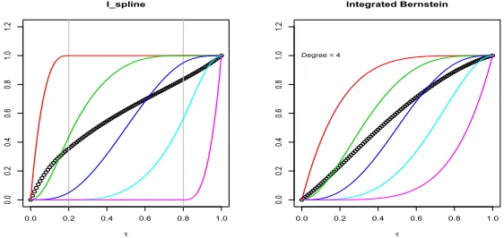
To achieve the monotonic properties, truncated power functions and polynomial basis
func-tions are widely used in the recent literature [Cai and Dunson, 2007; Reich et al., 2011]. For
instance, Bernstein basis polynomials bMm (τ) =
M m τ
m(1−τ)M−m reduce the
compli-cated monotonicity constraints to a sequence of simple constraints βm−βm−1 ≥ 0, for m =
2, ..., M[Reich et al., 2011]. Alternatively, we plot the I-splines and integrated Bernstein basis
polynomials IbMm(τ) = PM+1
k=m+1M1+1b
M+1
k (τ) for m = 0,1, ..., M with constraints βm ≥ 0 in Figure 2.1. Polynomials do have a limitation: changing the behavior ofβ(τ,Bs) near one value (τ1) has radical implications for its behavior for any other value (τ2) [Ramsay, 1988]. Thus,
when M is small, the polynomial transformation will be dominated by the central portion of
the distribution, and might behave unsatisfactorily in the tails. Choosing a largeM helps but
the computing burden becomes heavy (see Figure 2.1). This poses the problem of how to retain
flexibility, while leaving the function constrained at different percentiles as desired.
0.0 0.2 0.4 0.6 0.8 1.0
0.0 0.2 0.4 0.6 0.8 1.0 1.2 I_spline τ
0.0 0.2 0.4 0.6 0.8 1.0
0.0 0.2 0.4 0.6 0.8 1.0 1.2 Integrated Bernstein τ
Degree = 4
Figure 2.1: The comparison between the I-splines of order h=3 and the integrated Bernstein polyno-mials of degree 4. The I-splines are defined on [0, 1] and are associated with interior knots 0.2, 0.8. Each I-spline is piecewise cubic, and a monotonic curve is obtained by the linear combination of theseM=5 splines with nonnegative coefficients. The I-spline function is used to ensure the non-crossing quantiles with both flexibility and constrains at different percentiles.
ba-sis function from polynomials joined end-to-end. Particularly if compared with the Bernstein
polynomials, the integral of non-negative functions make the monotonicity constrains easier
to impose. The piecewise polynomial function is not only defined to ensure the non-crossing
quantiles, but also keeps the upper/lower tails in isolation from each other. In this paper, we
model the function I using the monotone spline regression. More specifically, we focus on the
integrated splinesIm, or I-splines for the sake of brevity [Lu and Clarkson, 1999; Ramsay, 1988].
For a simpleknot sequence {γ1, ..., γM+h},M is the number of free parameters that specify the spline function having the specified continuity characteristics, and h is the degree of the
piecewise polynomialIm. For allτ, there existsmsuch thatγm≤τ < γm+1. For application to
the important case where h=3, let: I1∗ = (τ −γm) (γm+2−γm+1)
;I2∗ = (τ −γm+1)
2−
(γm+3−τ)2
(γm+3−γm+1) (γm+2−γm+1);
I3∗ = (γm+3−τ)
3
(γm+3−γm+1) (γm+3−γm) (γm+2−γm+1)
-(τ−γm)3
(γm+3−γm) (γm+2−γm) (γm+2−γm+1).
The I-spline Im will be piecewise cubic, with zero for τ < γm and unity for τ ≥γm+3, with
the direct expressions:
Im(τ|γ) =
0, ifτ < γm (τ −γm)3
(γm+1−γm) (γm+2−γm) (γm+3−γm), ifγm
≤τ < γm+1
I1∗+I2∗+I3∗, ifγm+1 ≤τ < γm+2
1− (γm+3−τ)
3
(γm+3−γm+2) (γm+3−γm+1) (γm+3−γm), ifγm+2 ≤τ < γm+3
1, ifτ ≥γm+3
(2.3)
Because the I-spline is an integral of nonnegative splines, it yields monotone functions PM m=1
Im(τ)βm(Bs) when combined with nonnegative values of the coefficients βm(Bs) (see Figure
2.1).
take:
βm(Bs) =
βm∗ (Bs) ifβm∗ (Bs)≥0 0 otherwise
(2.4)
Therefore a model using β˜(Bs) induces via (2.2) a quantile process of QZ(τ|Bs). Without loss of generality, we choose the knots series withinγ1 = 0 andγM+h= 1. The quantile process thus satisfies the boundary conditions:
QZ(0|Bs) =β0(Bs), QZ(1|Bs) =β0(Bs) + M
X
m=1
βm(Bs) (2.5)
Here, we rescale the model output such that the range of Z over the grid cells belongs to
[0,1]. In addition, assume βm∗ (Bs) have prior βm∗ (Bs) ∼ N(µm,Σm), with Σm(Bs,B0
s) = σ
2
mB
exp (−||s−s0||/ρmB). The full conditional distribution of π(βm(Bs)|Z) are then given by f(Z|βm(Bs), βm∗(Bs))π(βm(Bs) |βm∗(Bs)) π(βm∗ (Bs)), and is obtained using the Metropolis-Hastings algorithm for further calibration.
2.1.2 Estimation
In this section we obtain the likelihood function of the model output using the quantile function.
Given the probability of the threshold exceedance δ, we have qZ(τ) = PMm=1Im(τ)βm +β0
be the underlying quantile process of z1, ..., zT given a grid cell Bs. Suppose z(1)..., z(l−1)<
β0+
P
mIm(δ)βm ≤z(l)...≤ z(u) ≤β0+
P
mIm(1−δ)βm <z(u+1), ...,z(T), whereqZ(τz(l)) =
z(l), qZ(τz(u)) = z(u). Then the probability density function of Z ∈ [qZ(τz(l)), qZ(τz(u))] is
obtained usingqZ(τ):
fZ
qZ(τz(i))
=fZ z(i)
= 1
∂qZ(τ) ∂τ
|τ=τ(z
where τzt solves zt=qZ(τzt) inτ, for t= 1,2, ..., T. Let τ1,τ2,..., τK denote K = 101 equally
spaced quantile levels in [0,1], a solution τzt to qZ(τzt|Z)−zt= 0 can be efficiently obtained
using Newton’s Recursion method [Tokdar and Kadane, 2011]:
τz(tk+1)=τz(tk)−qZ(τ
(k)
zt )−zt
∂ ∂τqZ(τ
(k)
zt )
, (2.7)
where τz(0)t is the initial value defined as the lower bound of the estimated quantile interval
containingz, i.e.,τz(0)t =
PK
k=1τk1I (τk≤z < τk+1). However, the output data which are outside
of [qZ(τz(l)), qZ(τz(u))] cannot be obtained directly by the quantile functions; how to specify the
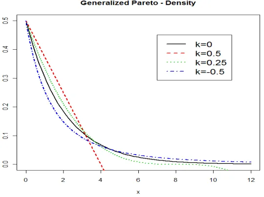
density at extreme values has been studied in the recent literature. A widely used approach to characterize such tail behavior is through the generalized Pareto distribution whose density
function is [Hosking and Wallis, 1987]:
ϕZ(z) = ω(1−κωz)1/κ−1, κ6= 0
= ωexp (−ωz), κ= 0. (2.8)
the range of z is 0≤z <∞ for κ≤0 and 0≤z≤1/(ωκ) forκ >0. Consequently, quantiles of the generalized Pareto distribution are given by:
qZ(τ) = (1−(1−τ)κ)/(ωκ), κ6= 0
= −log (1−τ)/ω, κ= 0. (2.9)
where the parameter rangesκ >0,κ= 0, andκ <0 correspond to the short tails, exponential
type and long tails, respectively. Note that the exponential distribution is a special case of
a generalized Pareto distribution with κ = 0 (see Figure 2.2). Therefore, in practice, the
generalized Pareto distribution is used in which some robustness is required against heavier
Figure 2.2: The probability density function for the generalized Pareto distribution is plotted with respect to the different tail index parameters κ. The parameter ranges κ > 0, κ = 0, and κ < 0 correspond to the short tails, exponential type and long tails, respectively.
Subsequently, given the tail index parameter κ, the likelihood function of Z is defined by a mixture distribution with its central part (2.6) and tails (4.6), such that:
fZ(z) =
CLϕZ
qZ(τz(l))−z;ωL
, ifz < qZ(τz(l))
1 ∂qZ(τ)
∂τ
|τ=τ(z), ifqZ(τz(l))≤z≤qZ(τz(u))
CUϕZ
z−qZ(τz(u));ωU
, ifz > qZ(τz(u))
(2.10)
where CL =τ(z(l)), CU = 1−τ(z(u)), ωL = 1 ∂qZ(τ)
∂τ
|τ=τ(z
(l))
CL , and ωU =
1 ∂qZ(τ)
∂τ
|τ=τ(z
(u))
CU . To
evaluate the likelihood, we use Markov chain Monte Carlo to sample from and summarize the
2.2
Spatial-temporal quantile regression
If we denote time with t, t=1,2,...,T,ut=(ut1, ut2, ..., utJ)0. ut1 ≡1 and utj is the B-spline of t with df=J-1, j=2,...,J. ThenQY(τ|ut, s) denotes theτth quantiles process of the observed daily
8-hour maximum ozone concentration at s and time t, while QZ(τ|ut, Bs) is the τth model
output quantile level for grid cell Bs given time t. Again, we relate the 12 km2 model output grid cell Bs to each monitoring sites.
We start by using quantile functions that vary with Bs,ut and τ for model output; thus,
they give a density regression model where the temporal trend is allowed to affect the shape of
the model output distribution. This means that:
QZ(τ|ut, Bs) =u0tβ0,Bs+βBs(τ) =
J
X
j=1
utjβ0j(Bs) +
M
X
m=1
Im(τ)βm(Bs), (2.11)
To specify monotonic constraints for QZ(τ|ut, Bs) with the temporal component ut, the
non-negativity ofβBs(τ) is required. More specifically, we introduce latent unconstrained variables
βm∗(Bs) and take constraints as (2.4) in section 2.1.1.
2.3
Simulation study
For nonparametric quantile regression, the proposed Bayesian spatial quantile method (BSQ)
is compared with the frequentist quantile regression method. In each example, L=100 data sets
are simulated. The data are given by:
z(ti,si)=f(ti,si) +g(ti,si)i (2.12)
• Example: Temporal quantile: f(ti,si) = 0.5 + 2ti+ sin(2πti−0.5), andg(ti,si)=1.
Model performance is evaluated in terms of the empirical root mean integrated squared
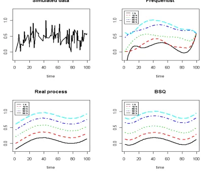
errorRM ISE = [T−1PT
t=1(ˆqz(τ|ut)−qz(τ|ut))2]1/2 forτ= 0.01, 0.5, 0.9 and 0.99. ˆqz(τ|ut) is the estimated function andqz(τ|ut) is the real function. The interior knots at (0.2, 0.8) provide a smaller RM ISE at the tails. In Figure 2.3, we plot a time series of the simulated data and
its underlying 100τth curve as the real process. The quantile spline regression captures most of the variations in the data but demonstrates a crossing problem. Our BSQ approach yields an
overall trend with a wide band.
Table 2.1: (Example 2) Empirical root mean integrated squared error (×100), with its standard error in parentheses
Method Knots δ τ = 0.01 τ = 0.50 τ = 0.90 τ = 0.99
BSQ (0.2, 0.8) 0.05 7.61(0.034) 5.11(0.014) 5.44(0.014) 7.07(0.030)
BSQ (0.3, 0.7) 0.005 7.84(0.029) 5.57(0.015) 6.77(0.018) 7.95(0.031)
Frequentist - - 15.80(0.038) 6.14(0.017) 8.51(0.030) 15.50(0.042)
2.4
Summary
In this chapter, we introduced a Bayesian framework for a simultaneous analysis of quantile
functions and quantile regression models. Because the frequentist method analyzes quantiles
separately, it is hard to provide a valid quantile function when taking the temporal effect into
account. Thus, constructing the quantile functions through a continuous quantile process is
essential to attain the true quantile framework, but there is a lack of computational efficiency
due to the associated monotonic constraints. Also, to obtain the non-fully specified likelihood,
we present a Bayesian density model based on the quantile functions. Tokdar and Kadane
extend it to deal with the unbounded variables. The resulting formulation leads to a mixture
distribution defined by both the 1−τ(z(l))−τ(z(u)) percentile of the data and a generalized
Pareto distribution for the tails. The simulation analysis presented in section 2.3 indicates the
Chapter 3
Spatial quantile calibration
As we discussed in Chapter 1, when linear regression is used for a data transformation problem,
there might be a strong desire to move beyond the most elementary type of transformation. In
this chapter, we consider only the model grid cells with a monitoring location, which allows us
to identify a calibration functionGτ to map the climate model quantile process to the quantile functions estimated by the observed monitoring data. Subsequently, a spatial adjustment of
the entire distribution of the model output with respect to the distribution of the monitoring
data is specified to downscale the calibration function and their spatial-quantile processes (See
Figure 4.1) . Finally, we incorporate a smoothed temporal trend in the calibration model to
handle the spatio-temporal calibration refer to the entire distribution.
3.1
Spatial quantile calibration of deterministic model output
For the purpose of calibrating the spatial-quantile process, we make use of a monotonically
increasing map ηs(τ,β˜Bs) as:
ηs(τ,βˆ˜Bs) =QZ(τ|Bs;
ˆ ˜
where βˆ˜Bs are sampled from the posterior distribution π(β˜Bs|Z). Thus we have the observed
quantiles of Y as follows:
QY (τ|s) =I
ηs(τ,βˆ˜Bs) 0
˜
α(s)=α0(s) +
M
X
m=1
Im
ηs(τ,βˆ˜Bs)
αm(s) (3.2)
where α˜(s) are spatially-varying coefficients. Similar to equation (2.4), we introduce a latent
unconstrained variableαm∗ (s) to ensure the quantile constraints:
αm(s) =
α∗m(s) ifα∗m(s)≥0 0 otherwise
(3.3)
αm∗ (s) are modeled as multivariate mean-zero Gaussian spatial processes with boundary con-ditions:
QY (0|s) =α0(s), QY (1|s) =α0(s) +
M
X
m=1
αm(s) (3.4)
However, strict bounds on Y may not be known a priori. To ensure that the posterior has a
proper distribution (see Appendix 1), we express the likelihood function as a mixture
distribu-tion similar to (4.5), i.e., forκ= 0:
fY(y) =
CLexp−ωL(α0−y)1I (y < α0)
× CUexp
−ωU(y−(α0+
X
αm))!1I(y > α0+ Σαm)
× (fY∗(y|s))1I(α0 ≤y≤α0+
X
αm)
(3.5)
whereωLandωU are positive rate parameters;CLandCU provide the probability of the left and right truncations. Additionally, fY∗ (y|s) is the density function derived from both the model output and observed quantile functions, and its computing algorithm is provided in Section 3.3.
include certain observed values. Also, we assume that there exist (M+1) independent Gaussian
processes α0(s), α1(s), ..., αM(s) such that, Cov (αm(s), αm(s0))=σms2 exp(−||s−s0||/ρms)
whereρms is the spatial decay parameter for the Gaussian process αm(s),m= 0,1, ..., M.
3.2
Spatial-temporal quantile calibration
The calibration model in section 3 can be extended to accommodate data collected over space
and time. When we want to calibrate the model output with respect to the monitoring data
for multiple years, it is necessary to take into account the effect of the temporal trend on the
distribution. If we denote time with t, t = 1,2, ..., T, ut=(ut1, ut2, ..., utJ)0. Let ut1 = 1 and
utj be the B-spline of t with df=J-1, j = 2, ..., J. ThenQY (τ|ut, s) denotes the τth quantile
process of the observed daily 8-hour maximum ozone concentrations at s and time t, while
QZ(τ|ut, Bs) is the τth model output quantile levels for grid cell Bs given time t. Again, we relate the model grid cellBs to each monitoring site s.
We start by using quantile functions that vary with Bs,ut and τ for model output. They
give us a density regression model where the temporal trend is allowed to affect the shape of
the model output distribution. This means that:
QZ(τ|ut, Bs) =ut0β0,Bs+βBs(τ) =
J
X
j=1
utjβ0j(Bs) +
M
X
m=1
Im(τ)βm(Bs) (3.6)
To specify monotonic constraints for QZ(τ|ut, Bs) with the temporal componentut, the
non-negativity ofβBs(τ) is required. More specifically, we introduce latent unconstrained variables
βm∗ (Bs) and take constraints as (2.4) in section 2.1.1.
In order to construct the quantile functions of Y based on the model output process, we
increasing maps from [0,1] onto itself given any location s:
ηut,s(τ,βˆ0,Bs,βˆBs) =QZ(τ|ut, Bs; ˆβ0,Bs,βˆBs) (3.7)
where ˆβ0,Bs ∝ π β0,Bs|Z
and ˆβBs ∝ π βBs|Z
. Then we have the quantiles of observed
dataY as follows:
QY (τ|ut, s) = ut0α0,s+αs
ηut,s(τ,βˆ0,Bs,βˆBs)
= J
X
j
utjα0j(s) + M
X
m Im
ηut,s(τ,βˆ0,Bs,βˆBs)
αm(s) (3.8)
We define the monotonic spatially-variantαm(s) as the following latent variables:
αm(s) =
α∗m(s) ifα∗m(s)≥0 0 otherwise
m= 1, ..., M (3.9)
as in section 3. We assume that there exist zero-mean Gaussian processes αm(s) such that,
Cov (αm(s), αm(s0)) =σms2exp (−||s−s0||/ρms) andρms is the spatial decay parameter for
the Gaussian processαm(s). The different temporal trends between model output and the ob-served quantile process are then adjusted through the calibration parametersα0(s), α1(s), ..., αm(s).
3.3
Estimation
In this section, we focus on how to obtain the likelihood for the monitoring data based only on
its quantile processQY (τ|s) =I
ηs(τ,βˆ˜Bs) 0
˜
α(s) and the model output predictive quantile
ηs(τ,βˆ˜Bs). Suppose the constraints (2.4) and (3.3) are satisfied, then τ → QY (τ|s) is
density forY in the form [Tokdar and Kadane, 2011]:
fY (y|s) = ∂ 1 ∂τQY(τ|s)
|τ=τZ,s(y) (3.10)
whereτZ,s(y) is the solution toy =QY (τ|s) in τ. We apply the truncated likelihood (3.5) to approximate the density function:
fY(y|s) =
CLexp−ωL(α0−y)
1I(y < α0)
× CUexp
−ωU(y−(α0+
X
αm))
!1I(y > α0+ X
αm)
×
1 ∂
∂τQY(τ|s)
|τ=τZ,s(y)
1I(α0 ≤y≤α0+
X
αm)
(3.11)
whenα0 ≤y≤α0+Pαm, the partial log-likelihood function offY∗ (y|s), over the monotonicity restrictions of (ηs,α(s)) is defined as:
X
i
logfY∗ (yi|s) = −X i
log ∂
∂τQY (τ|s)|τ=τZ,s(yi)
= −X
i
log ∂QY (τ|s) ∂ηs(τ,βˆ˜Bs)
·∂ηs(τ, ˆ ˜
βBs)
∂τ |τ=τZ,s(yi) (3.12)
whereτZ,s(yi) is the solution toyi =QY (τ|s), i= 1,2, ..., n. A solutionτZ,s(y) toQY (τ|s)−
y= 0 can be efficiently obtained using Newton’s Recursion method:
τZ,(ks+1)(y) =τs(k)(y)−
QY(τ
(k)
s (y)|s)−y
∂ ∂τQY(τ
(k)
s (y)|s)
where τZ,(0)s is an initial value in [0,1]. The evaluations of QY (τ|s) and ∂τ∂ QY (τ|s) at various values ofτ ∈[0,1] can be done by:
∂
∂τQY (τ|s) = ∂ ∂ηs
QY(τ|s)· ∂ ∂τηs
= M X m=1 ∂ ∂ηs Im
ηs(τZ,s(y),βˆ˜Bs)
αm(s)
! · M X m=1 ∂
∂τIm(τZ,s(y)) ˆβm(s)
!
To simplify the notation, let D∗1 = (γ 3
m+2−γm+1); D
∗
2 =
−3(γm+3−η)2
(γm+3−γm+1)(γm+3−γm)(γm+2−γm+1)
+ (γ −3(η−γm)2
m+3−γm)(γm+2−γm)(γm+2−γm+1). Then the derivative of the I-spline,
∂
∂ηIm(η(·)) consists of quadratic segments as follows:
∂
∂ηIm(η|γ) =
0, ifη < γm
3(η−γm)2
(γm+1−γm)(γm+2−γm)(γm+3−γm), ifγm ≤η < γm+1
D∗1+D∗2, ifγm+1≤η < γm+2 3(γm+3−η)2
(γm+3−γm+2)(γm+3−γm+1)(γm+3−γm), ifγm+2≤η < γm+3
0, ifη≥γm+3
(3.14)
The steps given in equations (3.12) and (3.14) provide a computationally feasible algorithm and
can efficiently be ran in a PC or laptop. This algorithm depends on the number of observations,
the number of grid points and the power of a computer. On a laptop computer with a 2.0 GHz
Intel Core 2 Duo processor and 4 GB memory, it takes several days for calibrating the eastern
3.4
Application: calibration of eastern US ozone data
3.4.1 Data description
We use maximum daily 8-hour average ozone concentrations in parts per billion (ppb) from
ns = 68 sites covering the eastern U.S. from May, 1st, 2002 to September, 30th 2002 (T=153), which were obtained from the EPA Air Quality System (AQS) and can be acquired from the
following website: http://www.epa.gov/ttn/airs/airsaqs/index.htm.
Another source of data is the 2002 base-run simulations from the Community Multiscale Air
Quality (CMAQ) model. CMAQ is a multi-pollutant, multi-scale air quality model that uses
state-of-the science techniques for simulating all atmospheric and land processes that affect the
transport, transformation, and deposition of atmospheric pollutants and their precursors on
both regional and urban scales. It is designed as a modeling tool for handling all the major
pol-lutant issues based on a whole atmosphere approach. In this study, four annual (2002 to 2005)
CMAQ model runs were completed over the eastern U.S. using a 12 km by 12 km horizontal
grid. We use the ozone monitoring stations as the spatial unit and extract climate data from
the grid cell containing the ozone monitoring station. Additional information and a complete
technical description of the CMAQ model are given by Byun and Schere [2006].
The range of the CMAQ forecast data is quite similar to the range of the ground level ozone
monitoring data. To compare the CMAQ forecasts with the observed monitoring data, we
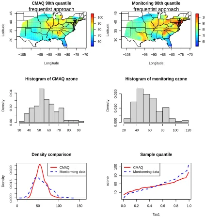
plot the sample quantile levels for the 90th percentile for our data sets over U.S. in Figure 4.4. Specifically, we extract data from a randomly selected site (the 59thsite is marked on the map as ∗), and investigate the histogram, sample quantile and density function of both observed and CMAQ data on this site. The observed ozone data have a heavier tail than the CMAQ
are unknown discrepancies in the CMAQ forecasts and an appropriate calibration is needed.
3.4.2 Result analysis and discussion
To compare spatial surfaces and distributions between the observed data and the CMAQ
out-put, we choose two data sources in the eastern U.S. We use the Metropolis-Hastings algorithm
for updating π(β˜, ρmB, σm2B|Z), π(α˜, ρms, σ2ms|Y, Z) individually. The likelihood is calculated by the likelihood approximation approach ofQY(τ|s) on a grid of 101 equally-spacedτk∈[0,1]. The I-splines have interior knots at (0.2, 0.8).
The estimated CMAQ quantiles and the calibration for the monitoring data are plotted in
Figure 3.3. Both of the two spatial-quantile processes are obtained by our Bayesian algorithm.
At τ= 0.05, 0.5, and 0.95, the empirical root mean integrated squared error is calculated as:
RM ISE= [n−1s ns
X
i=1
( ˆQZ(τ|Bsi)−QYˆ (τ|si)) 2]1/2
TheRM ISEat the 50thquantile is equal to 7.13, while the value is 13.17 for the 5th percentile and 15.46 for the 95th percentile, respectively. The results show the agreement between the distributions of the CMAQ output and the monitoring data at their median level, but show
large differences for the tails. Also, from the contour plot, we conclude that the CMAQ data
are smoother than the observed spatial structure, indicating that the physically based
numer-ical models cannot capture both the extreme values and spatial correlations that are in the
monitoring data.
Due to these differences, it is critical to calibrate the CMAQ data considering its
spatial-quantile structure. Based on the estimated CMAQ-monitoring calibration model, a nonlinear
where αˆ˜ are the posterior estimations. Then we rescaleGτ,s(z(t,Bs),αˆ˜) to its original range
(see Figure 3.4). We calculate ˆQY(τ|si) (the estimated quantiles of the monitoring data), ˜
QSZ(τ|si) (the quantiles of the Bayesian calibrated data), ˜QLZ(τ|si) (the quantiles from the
linear regression model) and ˜QLS(τ|si) (the quantiles from the scale model), atτ ∈[0.01,0.97]
and locationsi. The scale predictor is defined as:
ˆ
y(t,si) =y(·,si) + ˆα∗(z(t,Bsi)−z(·,Bsi))
where the scalar ˆα=
q
Var(y(t,si)−y(·,si))/Var(z(t,Bsi)−z(·,Bsi))).
The root mean squared error RM SE( ˆQ,q|˜si) = [K−1PKk=1( ˆQ(τk,si)−q˜(τk,si))2]1/2 is calculated for both the linear regression method and our Bayesian approach at each location
si. Figure 3.6 shows maps of the above quantiles whenτ = 0.95, and we use the difference root mean squared error:
DRM SE =n−1s ns
X
i=1
RM SE( ˆQY(τ|si),Q˜SZ(τ|si))−RM SE( ˆQY(τ|si),Q˜LZ(τ|si))
RM SE( ˆQY(τ|si),Q˜LZ(τ|si))
The DRMSE between the linear regression method and the quantile calibration method range
from -77% to 66%, and is -50.23% on average. The results show that 57 out of 68 (83.8%)
sites have a reduced RMSE using the Bayesian calibration method (i.e., Figure 3.4). The mean
DRMSE between the scale method and the quantile calibration method is -20.6%. The p-value
of a Two-sample Kolmogorov-Smirnov test between the observed data and the scale calibration
is 2.45e−11(Figure 3.5), while the p-value is equal to 0.454 for the Bayesian calibration. Thus
we do not reject the null hypothesis that the quantile calibrated series has the same distribution
as the observed data. We also obtain the Kolmogorov-Smirnov tests for Bayesian calibration
Vs. LM calibration (p-value: 0.0037) and Bayesian calibration Vs. Scale calibration (p-value:
In summary, the spatial-quantile calibration provides a platform to transform the different
parts of the model output distribution to the corresponding parts of the observed distribution
at different rates. As we expected, the performance of the calibrated CMAQ model data is
Climate Model Outputs
Model Output Quantile Process
𝑍(1,𝑩𝒔𝟏)
𝑍(𝑇,𝑩𝒔𝒏
𝒔) 𝑍(2,𝑩𝒔𝟐)
.
.
.
Quantile Process For Climate Model Outputs
𝑄!(𝜏!|𝑩𝒔), 𝑄!(𝜏!|𝑩𝒔),… 𝑄!(𝜏!|𝑩𝒔)
Monitoring Quantile Process
Monitoring Data
𝑌(1,𝒔𝟏)
𝑌(2,𝒔𝟏)
𝑌(𝑇,𝒔𝟏)
.
.
.
Quantile Process For the Observed Data
𝑄!(𝜏!|𝒔), 𝑄!(𝜏!|𝒔),… 𝑄!(𝜏!|𝒔) Calibration Function
𝑮(!,𝒔)
−105 −95 −90 −85 −80 −75 −70 30 35 40 45 Longitude Latitude 60 70 80 90 100
*
CMAQ 90th quantile
frequentist approach
−105 −95 −90 −85 −80 −75 −70
30 35 40 45 Longitude Latitude 60 70 80 90 100
*
Monitoring 90th quantile
frequentist approach
Histogram of CMAQ ozone
Density
30 40 50 60 70 80 90
0.00
0.02
0.04
Histogram of monitoring ozone
Density
20 40 60 80 100 120
0.000
0.010
0.020
0 50 100 150
0.000 0.015 0.030 Density comparison Density CMAQ Monitorming data
0.0 0.2 0.4 0.6 0.8 1.0
40 60 80 100 Sample quantile Tau1 oz one CMAQ Monitorming data
Figure 3.2: Maps of the sample 90th quantile levels of the ozone concentrations for both the CMAQ
output and observations; At a randomly selected site (i.e., 59th) where we have T=153 observations; we