THE DEVELOPMENT OF INTEGRATED PLANNING AND SCHEDULING FRAMEWORK FOR DYNAMIC AND REACTIVE ENVIRONMENT OF COMPLEX
MANUFACTURING PROBLEM
(PEMBANGUNAN RANGKA KERJA PERANCANGAN DAN PENJADUALAN BERSEPADU BAGI MASALAH PEMBUATAN YANG KOMPLEKS UNTUK
PERSEKITARAN DINAMIK DAN REAKTIF)
ZALMIYAH BINTI ZAKARIA SAFAAI BIN DERIS
MUHAMAD RAZIB BIN OTHMAN SAFIE BIN MAT YATIM
RESEARCH VOT NO: 79105
Jabatan Kejuruteraan Perisian
Fakulti Sains Komputer dan Sistem Maklumat Universiti Teknologi Malaysia
ABSTRACT
ABSTRAK
TABLE OF CONTENTS
CHAPTER TITLE PAGE
ABSTRACT ii
ABSTRAK iii
TABLE OF CONTENTS iv
1 TOWARDS IMPLEMENTING REACTIVE SCHEDULING FOR JOB
SHOP PROBLEM 1
1.1 Abstract 1
1.2 Introduction 2
1.3 Motivation 2
1.4 Definition of the JSSP 4
1.5 Related Works 6
1.6 Dynamic JSSP 7
1.7 Genetic Algorithms 8
1.8 Issues and Challenges 9
1.9 Suggestion for Further Work 10
1.10 Conclusion 10
1.11 References 11
2 MODELING THE REAL WORLD MANUFACTURING PROCESSES
USING PETRI NETS 17
2.1 Abstract 17
2.2 Introduction 18
2.3 Manufacturing Problem 19
2.4 Problem Description 20
2.6 Petri Nets 22
2.7 Case Study 24
2.7.1 Machine Modeling 24
2.7.2 Process Modeling 27
2.8 Simulation Results 31
2.9 Future Work and Conclusion 31
2.10 Acknowledgement 32
2.11 References 32
3 OPERATING SEQUENCING USING MULTI-POPULATION DIRECTED
GENETIC ALGORITHMS 34
3.1 Abstract 34
3.2 Introduction 35
3.3 Approaches and Methods 35
3.4 Sequencing Constraints 36
3.5 Operation Sequence Coding 38
3.6 Fitness Function 40
3.7 GA Operators 40
3.8 Mutation 41
3.9 Crossover 42
3.10 Multi-population Directed Genetic Algorithms 42
3.11 Results and Discussion 44
3.12 Conclusion 46
3.13 Acknowledgement 46
3.14 References 47
4 OPERATING SEQUENCING USING MODIFIED PARTICLE SWARM
OPTIMIZATION 49
4.1 Abstract 49
4.2 Introduction 50
4.3 Approaches and Methods 50
4.4 Sequencing Constraints 51
4.6 Comparison to Genetic Algorithms 54
4.7 Operation Sequence Coding 55
4.8 Fitness Function 58
4.9 Results and Discussion 58
4.10 Conclusion 60
4.11 References 60
5 GENETIC MATCH-UP ALGORITHMS FOR DYNAMIC SCHEDULING
OF A REAL MANUFACTURING PROBLEM 63
5.1 Abstract 63
5.2 Introduction 63
5.3 The Problem 64
5.4 Current Practice in this Shop Floor 65
5.5 Problem Description 66
5.6 Literature Review 68
5.7 Proposed Algorithms 74
5.7.1 The Step in The First Phase 74
5.7.2 The Step in The Second Phase 74
5.7.3 The Step in The Third Phase 74
5.8 Current Achievement and Future Plan 79
5.9 Conclusion 79
CHAPTER 1
TOWARDS IMPLEMENTING REACTIVE SCHEDULING FOR JOB SHOP PROBLEM
1.1 Abstract
Most of the research literature concerning scheduling concentrates on the static problems, i.e problems where all input data is known and does not change over time. However, the real world scheduling problems are very seldom static. Events like machine breakdown or bottleneck in some situation impossible to predict. Dynamic scheduling is a research field, which take into consideration uncertainty and dynamic changes in the real world scheduling problem. This chapter gives an overview of the real problem occurred in the field of dynamic scheduling. Then we propose a hybrid genetic algorithm for solving the dynamic job shop problem.
Keywords
1.2 Introduction
Scheduling problem can be found in many different application areas, e.g. manufacturing, logistic, transportation, communication, sports, education, administration, etc. Main task of scheduling is the creation of schedules, which are temporal assignments of a set of activities to a set of resources subject to a set of constraints. Examples of scheduling constraints include deadlines (e.g., job i must be completed by time t), resource capacities (e.g., there are only two machine for drill), precedence constraints on the order of tasks (e.g., a leaf must be painted before it is assembled), and priorities on tasks (e.g., finish job j as soon as possible while meeting the other deadlines).
Many scheduling problems are difficult to solve [1]. It has been shown that many scheduling problems are NP-hard problem [2, 3, 4, 5, 6, 7, 8] - the time required to compute an optimal schedule increases exponentially with the size of the problem, meaning that with present-day algorithms even moderately sized problems cannot be solved to guaranteed optimality.
The rest of this chapter is organized as follows. In section 1.3, the current issues that motivate the research on this area are discussed. In Section 1.4, a detailed description of the Job Shop Scheduling Problem (JSSP) is given. Section 1.5 summarizes the research done concerning JSSP. Section 1.6 and 1.7 discussed the previous genetic algorithms research aimed at solving the dynamic JSSP. Section 1.8 describes the current issues and challenges in this research area. In section 1.9, summarized the future plans.
1.3 Motivation
optimal solution because it is impossible to consider all nodes in a large search space. This problem is also called generative in [10] and predictive in [11, 12]. The second problem is dynamic problem which related to the dynamic nature of the problems, where variables and constraints always change due to the development of an organization or emergence of certain type of events. This problem is also called revisions in [11] and reactive in [10, 12]. This problem is viewed as the reactive part of the system which monitors the execution of the schedule and copes with unexpected events (i.e., machine breakdowns, tool failures, order cancelation, due date changes, etc) [11].
The major criticism brought against the predictive mechanisms in practice is that the actual events on the shop floor can be considerably different compared to the one specified in the schedule due to the random interruptions (i.e., machine breakdowns, bottleneck, due date changes, order cancelations, etc.) [13, 14]. Thus an appropriate corrective action (or response) should be taken to improve the performance of the infeasible schedule [7, 10, 11, 12, 15, 16, 17]. Although reactive scheduling is of great importance in any scheduling system, most scheduling research has mainly focused on the construction of a good generative schedule from scratch without providing enough attention on the reactive control phase.
In industrial practice, the majority of scheduling systems address the reactive scheduling problem by making it the responsibility of the human scheduler to evaluate the implications of the unexpected events, and to adjust the generative schedule accordingly [10, 12]. However, the combinatorial complexity of the scheduling problem tends to overburden the human scheduler and may result in poor schedule performance.
1.4 Definition of the JSSP
A N × M job shop scheduling problem, hereafter referred to as the JSSP, consists of N jobs and M machines [8]. A job j consists of a sequence of operations Oj = (oj1, o j2,…,ojkj). Each
operation ojl is to be processed on a specific machine and has a specific processing time
τ
jl. Eachjob has at most one operation on each machine (capacity constraint). The processing order of the operations in job j must be the order specified in the sequence Oj. These sequences are often
called the technological constraints and also referred to as the precedence constraint. During processing each machine can process at most one operation at a time, and no preemption can take place; once processing of an operation has been started it must run until it has completed. In the following Cj will denote the end of processing time of the last operation of job j in a given
schedule.
Some problems include a due date dj for each job, a time by which the processing of the
job is supposed to be finished, a release time rj for each job, prior to which no processing of the
job can be done, or a initial setup time sm for each machine, prior to which no processing can be
done on the machine.
A number of different objective functions exist for job shop problems. The most extensively researched is the makespan Cmax = maxj∈{1..N}(Cj), the time span needed to complete
all operations of all jobs. However the makespan objective is not well-suited for scheduling on a rolling time horizon-basis (jobs arriving continuously over time), and it does not include due
dates. More realistic objectives include total flowtime N1 j j j
F=
∑
= C −r , summed lateness1 N
j j
j
LΣ C d
=
=
∑
− , summed tardiness1max ( , 0) N
j j
j
TΣ C d
=
=
∑
− , maximum lateness Lmax =maxj∈{1..N}(Cj - dj) and maximum tardiness Tmax = max (Lmax, 0). All of these performance
Table 1.1 : A 3 × 3 problem
job Operations routing (processing
time)
1 1 (3) 2 (3) 3 (3)
2 1 (2) 3 (3) 2 (4)
3 2 (3) 1 (2) 3 (1)
An example of a 3 × 3 JSSP is given in Table 1.1. The data includes the routing of each job through each machine and the processing time for each operation (in parentheses). Figure 1.1 shows a solution for the problem represented by "Gantt-Chart".
M1
M2
M3
d
Figure 1.1: A schedule for a 3 x 3 JSSP instance
Based on the release times of jobs, JSSP can be classified as static or dynamic scheduling. In static JSSP, all jobs are ready to start at time zero. In dynamic JSSP, job release times are not fixed at a single point, that is, jobs arrive at various times. Dynamic JSSP can be further classified as deterministic or stochastic based on the manner of specification of the job release times. Deterministic JSSP assume that the job release times are known in advance. In stochastic JSSP, job release times are random variables and some or all parameters are uncertain [3, 5].
1.5 Related Works
As discussed earlier, the majority of the published literature in the scheduling area deals with the task of schedule generation or predictive nature of the scheduling problems. The normally employed approaches for the solution of these problems are heuristic strategies [4]. Some of the most common techniques used are branch and bound [19], dispatching rules [20, 21], tabu search [22, 23, 24, 25, 26], simulated annealing [27, 28, 29] and genetic algorithms [2, 3, 5, 7, 8, 17, 30, 31, 32, 33]. In [34] and [35] we can found an extensive study about the main techniques that were applied since the year 1960s. The application of GA to scheduling problems has interested many researchers due to the fact that they seem to offer the ability to cope with the huge search spaces involved in optimizing schedules.
However, reactive scheduling is also important for the successful implementation of scheduling systems. A review on research papers that are related to reactive scheduling was given in [11]. This chapter gives a short classification and a brief description about the existing studies concerning reactive scheduling.
Another popular approach to deal with reactive scheduling is knowledge-based system or expert system [14, 32, 36, 37, 38, 39, 40, 41, 42].
As stated earlier the common practice related to reactive scheduling in industrial practice is to assign human schedulers to repair the schedules using their knowledge and experience in the particular domain. This scenario shows that knowledge and experience are the most important elements to make the scheduling system become reactive because knowledge can provide information on where jobs are, where they need to go and what machine are up or down, etc.
Shah et al. [44] developed knowledge based dynamic scheduling for production of parts in a steel plant. A rule base is used to handle the shared transporter, moving components and treated in sequence stations.
1.6 Dynamic JSSP
Dynamic problems have been considered on a rolling time horizon basis, in which the problem is solved by making a schedule for the part of the problem that is known. Processing of the jobs according to this schedule is then started, and as soon as information about new jobs arrive a new schedule incorporating the new jobs and the work not yet processed in the previous schedule is created.
Most research on scheduling has been focused mainly on optimizing one particular performance measure, like the use of resources, makespan or tardiness, normally reflecting some kind of cost. It is assumed that all problem data are known before scheduling has to take place and no change ever happens. However real world applications operate in dynamic environments frequently subject to several kinds of random occurrences and perturbations, such as new job arrivals, machine breakdowns, employees sickness, jobs cancellation and due date and time processing changes, causing that the original schedule becomes unfeasible.
Due to their dynamic nature, real scheduling problems have an additional complexity in relation to static ones. In many situations these problems, even for apparently simple situations, are hard to solve, i.e. the time required to compute an optimal solution increases exponentially with the size of the problem [6].
The algorithms for dynamic scheduling should be able to manage any disruption of a schedule caused by changes in scheduling environment. Such changes can be classified in three major groups [16] :
• Activity Changes
Request for new or extended activities can result in resource contention and inconsistency of a schedule. In long term scheduling introducing new activities can aim at improving the schedule efficiency and degree of resource utilization (e.g. leasing out some resource leads). In the short term scheduling activities are introduced as they arise (e.g. emergency service). Changes in activity duration and increased level of resource usage can occur.
• Resource Changes
Primary reduction of resources (e.g. machine failure) can disrupt a schedule. Resource changes may be also requested to reduce the cost of a schedule (e.g. machine utilization problems). Shorter term resource changes are usually connected with resource failure.
• Temporal Changes
The most frequent form of temporal change is a contraction of schedule horizon. Long term temporal changes (e.g. changing a schedule in public transport for regularity) and short time changes (e.g. downstream effect of delayed aircraft or train) may also cause schedule inconsistency.
1.7 Genetic Algorithms (GA)
arrive at some known (deterministic JSSP) or unknown (stochastic JSSP) future times. Further, the importance of each job can be different and the objective is more complex [3].
1.8 Issues and Challenges
Although scheduling is a well researched area, and numerous articles and books have been published, classical scheduling theory has been little used in real production environments [45]. It is believed that scheduling research has much to offer industry and commerce, but that more work is needed to address the ‘gap’ between scheduling theory and practice [14, 46]. One frequent assumption of scheduling theory, which rarely holds in practice, is that the scheduling environment is static. In recent years many authors [7, 10, 11, 12, 13, 14, 15, 16, 17, 46] have recognized that this is unlikely scenario in many manufacturing environment. In reality, schedules must be revised frequently in response to both instantaneous events, which occur without warning, and anticipated events where information is given in advance by, for example, process control computers or customers.
As a consequence, even though GA have previously been demonstrated to have an acceptable performance on job shop problems, it is still have not been adopted in standard manufacturing practice. For this reason, in recent years, academic research has attempted to consider real-life scheduling problems. Standard benchmark problems do not attract the attention of people in industry since practical scheduling problems are far more complex than the famous benchmark problems [4] that are still used in most research.
For the comprehensive comparison and summary of results that have been published for the Lawrence’s [47] and Fisher and Thompson’s [6] benchmark problems see [4].
scheduling problem in a steel-making company using a hybrid system based on evolutionary algorithms and expert systems. Shaw and Fleming [51] and Kumar and Srinivasan [52] proposed evolutionary computation methods for the solution of scheduling problems in companies that produce ready-chill meals and defense products, respectively. Sakawa et al. [53] considered the scheduling problem of a machining center using an evolutionary algorithm. Shah et al. [44] developed knowledge based dynamic scheduling for Steel Plant. Finally, Suh et al. 1998 [10] implemented ordering strategies for constraint satisfaction in steel industry. A scheduling expert system was developed to implement these strategies for the reactive adjustment of hot-rolling schedules in a hot strip mill.
1.9 Suggestion for Further Work
We propose to use GA with a match-up approach to solve dynamic problem in the job shop scheduling problem. GA was chosen since it is well suited to optimization problem and were proved successfully solve a number of problem that were difficult to solve with other methods [32]. We proposed to use match-up approach in order to change only a part of the initial schedule when a disturbance occurs, in such a way as to accommodate new disturbances and maintain both performance and stability of the shop floor. In order to make this JSSP realistic to the real world problem, we will use the real data from automotive spring production as a case study.
1.10 Conclusion
1.11 References
[1] Parker R. G. (1995) Deterministic Scheduling Theory, London, Chapman & Hall.
[2] Yamada T and Nakano R. Genetic Algorithms for Job-Shop Scheduling Problems. Proceedings of Modern Heuristic for Decision Support, UNICOM seminar, 18-19 March 1997, London, pp. 67-81.
[3] Lin S., Goodman E.D. and Punch W. F. A Genetic Algorithm Approach to Dynamic Job Shop Scheduling Problems. International Conference of Genetic Algorithms (ICGA) 1997.
[4] Dimopoulos C. and Zalzala A.M.S. Recent developments in evolutionary computation for manufacturing optimization: problems, solutions, and comparisons. IEEE Transactions on Evolutionary Computation, Vol. 4, No. 2, July 2000 pp. 93 – 113.
[5] Madureira A. M., Ramos C. and Silva S. D. C. A Genetic Approach for Dynamic Job-Shop Scheduling Problems. 4th MetaHeuristics International Conference (MIC‘2001), Portugal, 2001.
[6] Blazewicz J, Ecker K.H., Pesch E, Schmidt G. and Weglarz J. Scheduling Computer and Manufacturing Processes, Springer, Berlin, 2001.
[7] Jensen M. T. Generating Robust and Flexible Job Shop Schedules using Genetic Algorithms. IEEE Transactions on Evolutionary Computation, Vol. 7, no 3, June 2003, pp. 275-288.
[8] Braune R., Wagner S. and Affenzeller M. Applying Genetic Algorithms to the Optimization of Production Planning. Real-World Manufacturing Environment, Cybernetics and Systems, 2004.
[10] Suh M. S., Lee A., Lee Y. J. and Ko Y. K. Evaluation of ordering strategies for constraint satisfaction reactive scheduling. Decision Support Systems, Vol. 22, Issue 2, Feb. 1998, pp. 187-197.
[11] Sabuncuoglu I. and Bayiz M. Analysis of reactive scheduling problems in a job shop environment. European Journal of Operational Research, Vol. 126, Issue 3, Nov. 2000, pp. 567-586.
[12] Sauer J. Planning and Scheduling - An Overview. in: Hotz, L., Krebs, T. (Eds.): Planen und Konfigurieren (PuK-2003), Proceedings des Workshops zur KI 2003, Hamburg, 2003, pp. 158-161.
[13] Akturk, M. S. and Gorgulu, E., Match-up scheduling under a machine breakdown, European Journal of Operational Research, Vol. 112, Issue 1, Jan. 1999, pp. 81-97.
[14] Cowling P. and Johansson M., Using real time information for effective dynamic scheduling, European Journal of Operational Research, Vol. 139, Issue 2, June 2002, pp. 230-244.
[15] Dorn, J. Case-based reactive scheduling. in Roger Kerr and Elisabeth Szelke (eds) Artificial Intelligence in Reactive Scheduling. London: Chapman & Hall. 1995, pp. 32-50.
[16] Kocjan W. Dynamic scheduling: State of the art report. Technical Report T2002:28, SICS, 2002.
[17] Vazquez M. and Whitley L. D. A comparison of genetic algorithms for the dynamic job shop scheduling problem. Proceedings of GECCO-2000, 2000, pp. 169-178.
[18] Graves S.C. A review of production scheduling, Operations Research, Vol. 29, Issue 4, 1981, pp. 646-675.
[19] Carlier J. and Pinson E. An Algorithm for Solving the Job-Shop Problem. Management Science, Vol. 35, 1989, pp. 164-176.
[21] Lodree E. J., Jang W., Klein C. M. A new rule for minimizing the number of tardy jobs in dynamic flow shops. European Journal of Operational Research 159, 2004, 258-263.
[22] Hurink J. and Knust S., A tabu search algorithm for scheduling a single robot in a job-shop environment, Discrete Applied Mathematics, Vol. 119, Issues 1-2, June 2002, pp. 181-203.
[23] Watson J. P., Beck J. C., Howe A. E. and Whitley L. D. Problem difficulty for tabu search in job-shop scheduling, Artificial Intelligence, Vol. 143, Issue 2, Feb. 2003, pp. 189-217.
[24] Carotenuto P., Giordani S., Ricciardelli S. and Rismondo S., A tabu search approach for scheduling hazmat shipments. Computers & Operations Research, In Press, Corrected Proof, Available online 22 July 2005.
[25] Liu S.Q., Ong H.L. and Ng K.M., A fast tabu search algorithm for the group shop scheduling problem. Advances in Engineering Software, Vol. 36, Issue 8, Aug. 2005, pp. 533-539.
[26] Xu J., Sohoni M., McCleery M., Bailey T. G., A dynamic neighborhood based tabu search algorithm for real-world flight instructor scheduling problems. European Journal of Operational Research, Vol. 169, 2006, pp. 978–993.
[27] Mamalis A. G. and Malagardis I. Determination of due dates in job shop scheduling by simulated annealing. Computer Integrated Manufacturing Systems, Vol. 9, Issue 2, May 1996, pp. 65-72.
[28] Satake T., Morikawa K., Takahashi K. and Nakamura N. Simulated annealing approach for minimizing the makespan of the general job-shop. International Journal of Production Economics, Vol. 60-61, April 1999, pp. 515-522.
[30] Fang H.L., Ross P., Corne D., A promising genetic algorithm approach to job-shop scheduling, rescheduling, and open-shop scheduling problems. Proceedings of the Fifth International Conference on Genetic Algorithms, 1993, pp. 375–382.
[31] Bierwirth C. and Mattfeld D.C. Production scheduling and rescheduling with genetic algorithms, Evolutionary Computation, Vol. 7, Issue 1, 1999, pp. 1–17.
[32] Varela R., Vela C.R., Puente J. and Gomez A. A knowledge-based evolutionary strategy for scheduling problems with bottlenecks. European Journal of Operational Research, Vol. 145, 2003, pp. 57–71.
[33] Goncalves J. F, de Magalhaes Mendes J. J., Resende M. G. C. A hybrid genetic algorithm for the job shop scheduling problem. European Journal of Operational Research, Vol. 167, 2005, pp. 77–95.
[34] Blazewicz J., Domschke W. and Pesch E. The job shop scheduling problem: Conventional and new solution techniques. European Journal of Operational Research, Vol. 93, 1996, pp. 1–33.
[35] Jain A.S., Meeran S., Deterministic job-shop scheduling: Past, present and future, European Journal of Operational Research, Vol. 113, 1999, pp. 390–434.
[36] Shah V. C., Madey G. R. and Mehrez A. A methodology for knowledge-based scheduling decision support, Omega, Vol. 20, Issues 5-6, Sept.-Nov. 1992, pp. 679-703.
[37] Collinot A. and Le Pape C. Adapting the behavior of a job-shop scheduling system. Decision Support Systems, Vol. 7, Issue 4, Nov. 1991, pp. 341-353.
[38] Ress D. A. and Currie K. R. Development of an expert system for scheduling work content in a job shop environment. Computers & Industrial Engineering, Vol. 25, Issue 1-4, Sept. 1993, pp. 131-134.
[40] Miyashita K. and Sycara K. CABINS: a framework of knowledge acquisition and iterative revision for schedule improvement and reactive repair. Artificial Intelligence, Vol. 76, Issues 1-2, July 1995, pp. 377-426.
[41] Zhang Y. and Chen H. A knowledge-based dynamic job-scheduling in low-volume / high-variety manufacturing. Artificial Intelligence in Engineering, Vol. 13, Issue 3, July 1999, pp. 241-249.
[42] Henning G. P. and Cerda J. Knowledge-based predictive and reactive scheduling in industrial environments. Computers & Chemical Engineering, Vol. 24, Issues 9-10, Oct. 2000, pp. 2315-2338.
[43] Szelke E. and Kerr R.M. Knowledge-based reactive scheduling, Production Planning and Control, Vol. 5, Issue 2, 1994, pp. 124-145.
[44] Shah M.J., Damian R., Silverman J. Knowledge Based Dynamic Scheduling in a Steel Plant. Proceedings of the 6th International Conference on Artificial Intelligence for Industrial Applications, St. Barbara, 1990, pp. 108-113.
[45] Stoop P. and Wiers V. The complexity of scheduling in practice. International Journal of Operations & Production Management, Vol. 16 No. 10, 1996, pp. 37-53.
[46] Aytug H., Lawley M. A., McKay K., Mohan S. and Uzsoy R. Executing production schedules in the face of uncertainties: A review and some future directions. European Journal of Operational Research, Vol. 161, Issue 1, Feb. 2005, pp. 86-110.
[47] Lawrence S., Resource Constrained Project Scheduling: An Experimental Investigation of Heuristic Scheduling Techniques. Pittsburgh, PA: GSIA, Carnegie Mellon Univ., 1984.
[49] Gilkinson J. C., Rabelo L. C., and Bush B. O., A real-world scheduling problem using genetic algorithms. Computers & Industrial Engineering, Vol. 29, Issue 1–4, 1995, pp. 177–181.
[50] Hamada K., Baba T., Sato K., and Yufu M. Hybridizing a genetic algorithm with rule-based reasoning for production planning. IEEE Expert, Vol. 10, No. 5, 1995, pp. 60–67.
[51] Shaw K. J. and Flemming P. J. Including real-life preferences in genetic algorithms to improve optimization of production schedules. Proc. Conf. Genetic Algorithms Eng. Syst.: Innovations and Appl.. Stevenage, U.K.: IEE, 1997, pp. 239–244. IEE Conf. Publ. 446.
[52] Kumar N. S. H. and Srinivasan G. A genetic algorithm for job-shop scheduling - A case study. Computer Industry, Vol. 31, no. 2, 1996, pp. 155–160.
[53] Sakawa M., Kato K. and Mori T. Flexible scheduling in a machining center through genetic algorithms. Computers & Industrial Engineering, Vol. 30, No. 4, September 1996, pp. 931-940.
CHAPTER 2
MODELING THE REAL WORLD MANUFACTURING PROCESSES USING PETRI NETS
2.1 Abstract
2.2 Introduction
Every company strives to increase their profits. One of the key factors in ensuring the profits is effective utilization of manufacturing resources through application of efficient planning and scheduling approaches. These two main approaches are closely related to the manufacturing processes in a flexible manufacturing system (FMS) which are formally known as process planning and production scheduling.
Process planning is refers to a process plan which is generated for each part to be manufactured in a manufacturing system [16]. The process plan specifies operations to be performed and their sequence, required resources and process parameters of each operation. On the other hand, production scheduling determines the most appropriate moment to execute each operation for the planned production, taking into account the due date, a maximum resource utilization, etc., in order to achieve high productivity in a manufacturing system [6]. One of the objectives of this work is to develop the process models, to help the definition of production processes. These models allow focusing on the second objective, which is to implement an integrated process planning, to specify the operations to be performed in manufacturing a product; and production scheduling, to estimate a start time for the particular operations to be performed in the case of manufacturing an automotive spring product. This chapter concentrates on the modeling of production processes using Petri Nets (PN) in order to understand the dynamic behavior of machine and production processes. Our case study is automotive spring production.
2.3 Manufacturing Problem
In essence, a manufacturing system can be viewed as a sequence of discrete events [4] or a discrete event dynamic system (DEDS) [7], i.e. a system with concurrency, mutual exclusions, decisions and synchronizations. In a typical time history of event, we would observe that more than one event could be occurring at the same time. From this time history we can identify the following characteristics [3]:
Concurrency or parallelism. In a manufacturing system many operations take place simultaneously.
Asynchronous operations. The evolution of system events is aperiodic. This may be due to
variable process completion times, e.g., the time to machine a part may vary from one part to another. In the case of the assembly of two different parts, one may be ready to be assembled before the other. Hence the two parts are being produced asynchronously.
Event driven. The completion of one operation may initiate more than one new operation.
Also, since there are other processes in the system, the order of occurrence of events is not necessarily unique.
As a result of these dynamic characteristics there are two other situations that can occur:
Deadlock. In this case, a state can be reached where none of the processes can continue. This
can happen with the sharing of two resources between two processes. This situation is undesirable and is usually the result of the system design. An important feature of a good model is that it can detect deadlock, permitting time for correction and redesign prior to system implementation.
Conflict. This may occur when two or more processes require a common resource at the same
There are many combinations of sequences of events that can occur in these systems. As a result, this can lead to a large state space. In order to solve this complexity, a modeling technique which able to contend with, and manage, the size of this state space is needed. Hence a modeling tool should model in detail the concurrency and synchronization in the system with respect to time. Furthermore, such a tool should help to analyze the system behavior to check for aspects such as deadlocks. Since it is very common in FMS to share certain resources (e.g. an operator is shared by more than one machine to load/unload), a modeling tool should represent these aspects to analyze the conflicts during the system execution.
Petri nets (PN) have all these capabilities and hence are suitable as dynamic modeling tool irrespective of the various methods used for modeling the dynamic behavior of FMS such as state diagrams [12], as well as state transition diagrams and interaction diagrams [2]. In object-oriented design, state diagrams or state transition diagrams are used to represent how objects respond to the internal and external events in the system. Interaction diagrams are used to study the synchronization aspects and to trace the execution of events in the system. Also, unlike previous works which use two different kinds of diagrams for representing system states and tracing events [2],[12], PN can be used as a single tool to represent both the system states and to trace the events in the system when time durations of activities are associated with transitions.
2.4 Problem Description
Automotive spring production is one of the discrete manufacturing which produces high variety of automotive spring products. Most of the automotive spring productions involve the difference product models that also need different processes.
quenching, and tempering. Likewise, assembly could be carried out through a sequence of operations include the part finishing processes such as bushing, painting, marking, and reverting; and then assembling the machined parts to form the required products. In this section the scheduling problems for manufacturing processes is defined.
2.5 The Scheduling Problem
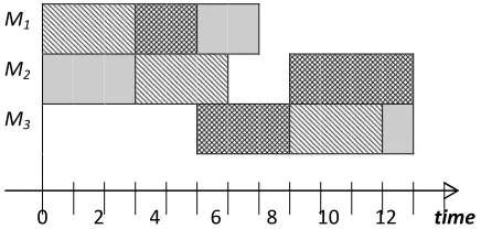
There are m dedicated machines at forming, heating and assembly stations. Thus, the problem is composed of m machines {M1, M2, …, Mm} and has n jobs (parts to be produced)
{J1, J2, …, Jn}. Each job Ji requires a sequence of operations {Oi1, Oi2…Oik}. The processing
time pik of each operation Oik is given. The objective of the scheduling is to determine the
operation sequences, determine the optimal route (machine) to process the parts, and estimate the start time of production activities, so that the makespan (Cmax), i.e., the maximum
completion time, is minimized, in the way that minimize machine idle time and balance machine load.
In this chapter, the process sequence of a product refers to the order in which parts or subassemblies are process by the machines. Here, the process sequence of a product to be produced is represented by a Petri nets which referred to as process model, which being discussed in details in next section.
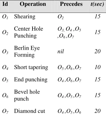
Table 2.1: Precedence constraints and processing time Id Operation Precedes t(sec)
O1 Shearing O2 15
O2
Center Hole Punching
O3, O4 ,O5
,O6 ,O7
15
O3
Berlin Eye
Forming nil 20
O4 Short tapering O5 ,O6 ,O7 10
O5 End punching O4 ,O6 ,O7 15
O6
Bevel hole
punch O4 ,O5 ,O7 15
O7 Diamond cut O4 ,O5 ,O6 20
For example, there is one model of product to be produced. This product consists of three main part components, namely leaf 1, leaf 2 and leaf 3, which involve distinct operations. In order to solve this scheduling problem, the processes related to this problem needs to be defined, as well as constraints. Each product consists of parts, and there are a number of operations to be performed on each part (see for example Figure 2.1).
The sequence of operations is bounded to the precedence constraints. Table 2.1 shows the precedence constraints for the forming processes. O04,…, O07 is a set of flexible-route
operations which can be performed in any order. These precedence constraints can be clearly viewed through the developed process model in the next section.
2.6 Petri Nets
A Petri net is a graphical and mathematical modeling tool for describing and studying systems that are characterized as being concurrent, asynchronous, distributed, parallel, stochastic and/or nondeterministic. Petri nets can be used as a visual-communication aid similar to flow charts, block diagrams, and networks. In addition, tokens are used in these nets to simulate the dynamic and concurrent activities of systems [8].
In PN modeling, there are two nodes [17], places and transitions, represented by circles and bars, respectively. The places are used to represent the status of a resource, e.g., its availability; a process, e.g., its undergoing; or condition, e.g., its satisfaction. The bars are used to model the events, e.g., start and end of an operation. A token is represented by a dot located in a place indicates weather a resource is available, a process is undergoing, or a condition is true. Multiple tokens often imply availability of multiple resources or the undergoing of operations of several parts. When the conditions for an event become all true, the corresponding transition is enabled and thus can fire. Firing enables the flow of tokens from places to places, implying the change of system status.
Formally, a Petri net can be defined as follows:
A Petri Net (PN) is a 5-tuple, PN = (P, T, I, O, M0) where [18]:
P = {p1, p2 … pm} is a finite set of places.
T = {t1, t2 … tn} is a finite set of transitions.
I : (P × T) → N is an input function that defines the directed arcs from places to transitions, where N is a set of non-negative integers.
O : (P × T) → N is an output function that defines the directed arcs from transitions to places M0 : P → N is the initial marking.
In order to simulate the dynamic behavior of the model, a state or marking represented by a token is changed according to the enabling and firing or transition rules [17]:
– Enabling Rule: A transition t is enabled if each input places have enough tokens : m(p) ≥ I(p,t), ∀ p ∈ P.
Firing happens by changing distribution of tokens on places, which reflect the occurrence of events or execution of operations. There are two stages of firing. First, remove the required number of tokens from each input place I and the number of tokens equals to the number of directed arc connecting p to t, which reflected by - I(p,t) in the equation above. Second, deposit tokens into each of output place p and the number of tokens equals to the number of directed arc connecting t to p, which represented by + O(p,t) in the equation.
2.7 Case Study
In order to assist us to understand the behavior of manufacturing process, we developed two PN models namely machine model and process model.
2.7.1 Machine Modeling
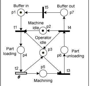
Figure 2.2: Machine modeling
Table 2.2: Detail Descriptions of Places for Machine Model
Place State
p1 Raw part are ready in buffer-in
p2 Machine available
p3 Operator available
p4 Part loaded ready for machining
p5 Part machining
p6 Finished part for unloading
p7 Finished part are ready in buffer-out
Figure 2.2 shows a machine model to illustrate this behavior. This model contains seven places denoted by p1, p2, p3, p4, p5, p6 and p7 and five transitions denoted by t1, t2, t3, t4
and t5. Its initial marking is the vector M0 = [1,1,1,0,0,0,0] represents the number of token in
the places. The time θ associated with timed transition t2 represents the processing time for
the machining operation. The tokens in place p1, p2 and p3 represent the availability of raw
material (part) waiting for operations, the machine and the operator waiting for serving the machine, respectively.
In this model, place p2 contains one token, which prevents t1 being fired twice
simultaneously. From a practical point of view, this means that the related machine cannot perform more than one operation at one time. This condition is also referred to as capacity constraints.
Table 2.2 and Table 2.3 show the detail descriptions of the places and transitions in this machine model, respectively.
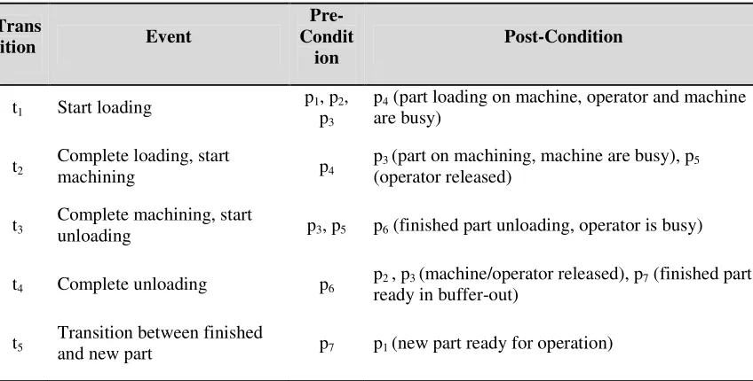
Table 2.3: Detail Descriptions of Transitions for Machine Model
Trans
ition Event
Pre-Condit
ion
Post-Condition
t1 Start loading
p1, p2,
p3
p4 (part loading on machine, operator and machine
are busy)
t2
Complete loading, start
machining p4
p3 (part on machining, machine are busy), p5
(operator released)
t3
Complete machining, start
unloading p3, p5 p6 (finished part unloading, operator is busy)
t4 Complete unloading p6
p2 , p3 (machine/operator released), p7 (finished part
ready in buffer-out)
t5
Transition between finished
and new part p7 p1 (new part ready for operation)
The dynamic behavior of the system can be observed through this model.
• Transition t1 represents the model of the start of loading a part by the operator. Initially
only transition t1 is enabled since only t1's enabled condition are met. Three arcs link from
p1, p2 and p3 to t1 meaning that three condition in p1, p2 and p3 have to be met before the
event in t1 can happen. Firing t1, removes three tokens from p1, p2 and p3, and deposits a
token to p4. Now, places p1, p2 and p3 hold no token and transition t1 is disabled. The
occurrence of event t1 allows the machine (operator) to enter the status of “being loading
with a part” (loading a part) modeled by place p2 (p3), respectively. Then, the loaded part
at p4 is ready for machining.
• Transition t2 model both “completion of operator’s loading” and “start of machining”.
One arc from p4 to t2 represents that t2’s being enabled if one conditions met. Now, only
transition t2 is enabled and firing t2, removes a token from p4 and deposits a token to p3
and p5 , respectively.
• Now, onlytransition t3 is enabled and firing t3, removes two tokens from p2 and p5 and
deposits a token to p6.
• Then, onlytransition t4 is enabled and firing t4, removes a token from p6 and deposits a
• Finally, onlytransition t5 is enabled and firing t5, removes a token from p7 and deposits a
token to p1. Now the system returns to the initial condition and ready to repeat the above
processes.
The machine model helps us to understand the behavior of the machine, served by the operator in order to process the parts. From this model, we develop the process model for the overall production processes.
2.7.2 Process Modeling
The process of manufacturing a product can be viewed as a sequence of operations, to be carried on a different machine. We have been developed a process model to represent the sequence of operations to be performed. A process model includes a set of activities or processes arranged in a specific order, with the clearly identified inputs and outputs. The input may be either a raw material or semi-finished part. Meanwhile the output maybe either a semi-finished part, sub-assembled or assembled product. Each activity in a process takes an input and transforms it into an output with some value added.
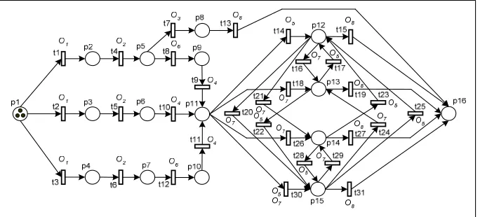
Figure 2.3 shows the process model for the previous example. In this model, each place represents the input and output buffer of the machine, each transition represents the operation performed by the machine, an arc represents a precedence relationship between two operations and a token represents the availability of a part.
The goal of process model is to demonstrate the dynamic behavior of production processes. The process model for the previous example contains sixteen places (p1, p2, …,
p16) and thirty one transitions (t1, t2, …, t31). The initial marking M0 =
[3,0,0,0,0,0,0,0,0,0,0,0,0,0,0,0]. The three tokens in p1 represent three raw materials (parts) to
be manufactured.
This process model is closely related to the previous machine model. The places p in this process model represents the operation Oi performed on a particular machine Mi. So the
Figure 2.3: Process modeling
The dynamic behavior of the system can be observed through this model:
• Initially, t1, t2, t3 are enabled. Firing t1, t2, t3 (shearing), removes three tokensfrom p1
and deposits a token to p2, p3, p4, respectively. Consequently, now p1 hold no token and
p2, p3, p4 hold one token, respectively.
• Now, M1 = [0,1,1,1,0,0,0,0,0,0,0,0,0,0,0,0], the three parts at p2, p3, p4 are on shearing. • Then t4, t5, t6 are enabled. Firing t4, t5, t6 (start of punching) removes a token from p2,
p3, p4, respectively, and deposits a token to p5, p7, p8, respectively. Now, p5, p7, p8 hold
one token, respectively.
• Now, M2 = [0,0,0,0,1,0,1,1,0,0,0,0,0,0,0,0], then 3 parts at p5, p7, p8 are on punching.
Then this simulation will be executed accordingly until the end of the process.
The arcs associated with p12 to p15 represent the most complex part of this model. The
complexity is due to the flexibility of the system. Thus, this complexity reflects the fact that the more flexible the route the more complex the model. In essence, p12 to p15 represent a set
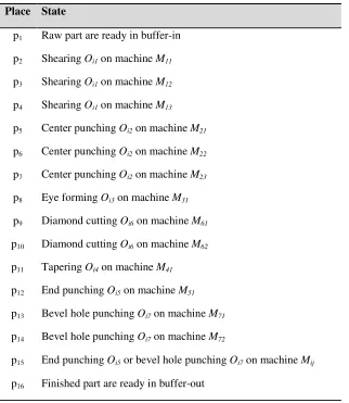
Table 2.4: Detail Descriptions of Places for Process Model. Place State
p1 Raw part are ready in buffer-in
p2 Shearing Oi1 on machine M11
p3 Shearing Oi1 on machine M12
p4 Shearing Oi1 on machine M13
p5 Center punching Oi2 on machine M21
p6 Center punching Oi2 on machine M22
p7 Center punching Oi2 on machine M23
p8 Eye forming Oi3 on machine M31
p9 Diamond cutting Oi6 on machine M61
p10 Diamond cutting Oi6 on machine M62
p11 Tapering Oi4 on machine M41
p12 End punching Oi5 on machine M51
p13 Bevel hole punching Oi7 on machine M71
p14 Bevel hole punching Oi7 on machine M72
p15 End punching Oi5 or bevel hole punching Oi7 on machine Mij
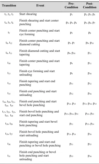
Table 2.5: Detail Descriptions of Transitions for Process Model
Transition Event
Pre-Condition
Post-Condition t1, t2, t3 Start shearing p1 p2, p3, p4
t4, t5, t6
Finish shearing and start center
punching p2, p3, p4 p5, p6, p7
t7
Finish center punching and start
eye forming p5 p8
t8, t12
Finish center punching and start
diamond cutting p5, p7 p9, p10
t9, t11
Finish diamond cutting and start
tapering p9, p10 p11
t10
Finish center punching and start
tapering p6 p11
t13
Finish eye forming and start
unloading p8 p16
t14
Finish tapering and start end
punching p11 p12
t15
Finish end punching and start
unloading p12 p16
t16, t20, t21,
t24, t29
Finish end punching and start
bevel hole punching p12, p15 p13, p14, p15 t17, t22, t23,
t25, t28
Finish bevel hole punching and
start end punching p13, p14, p15 p12, p15
t18, t26
Finish tapering and start bevel
hole punching p11 p13, p14
t19, t27
Finish bevel hole punching and
start unloading p13, p14 p16
t30
Finish tapering and start end
punching or bevel hole punching p11 p15
t31
Finish end punching or bevel hole punching and start unloading
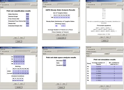
2.8 Simulation Results
To verify the proposed models we used PIPE2 (Platform Independent Petri Net Editor) [19] to edit, animate and analyze our models. Figure 2.4 shows some of the simulation results for the proposed models. The result shows the feasibility of our models.
Figure 2.4: Simulation Results using PIPE2
2.9 Future Work and Conclusion
and the scheduling of manufacturing system. We used the proposed models to help the definition of production processes. These models allow focusing on implementing an integrated process planning and production scheduling in the case of manufacturing the automotive spring product.
2.10 Acknowledgement
Special thanks are due to APM Automotive Holdings Bhd and Zilun System Sdn Bhd for the provided data.
2.11 Reference
[1] Aytug H., Lawley M. A., McKay K., Mohan S. and Uzsoy R. Executing production schedules in the face of uncertainties: A review and some future directions. European Journal of Operational Research, Vol. 161, Issue 1, Feb. 2005, pp. 86-110.
[2] Booch, G., Object-oriented analysis and design with applications. 1994 Reading, Mass. : Addison-Wesley.
[3] Cowling P. and Johansson M., Using real time information for effective dynamic scheduling, European Journal of Operational Research, Vol. 139, Issue 2, June 2002, pp. 230-244.
[4] Desrochers, A.A. and R.Y. Al-Jaar, Applications of petri nets in manufacturing systems : modeling, control, and performance analysis. 1995: Piscataway, N.J. : IEEE.
[5] Hestermann, C. and Wolber, M. (1997). A comparison between Operations Research-models and real world scheduling problems. The European Conference on Intelligent Management Systems in Operations, pp. 29-36. 25-26 March 1997. University of Salford, U.K.
[7] Malo-Tamayo, A., D. Gaviño-Contreras, and A. Ramíerez-Traviño, Petri net based control for the dynamic scheduling of a flexible manufacturing cell. IEEE International Conference on Systems, Man and Cybernetics 1998 1: p. 553-557.
[8] Murata, T., Petri nets: Properties, analysis and applications. Proceedings of the IEEE, 1989. 77(4): p. 541-580.
[9] Parker R. G. (1995) Deterministic Scheduling Theory, London, Chapman & Hall.
[10] Pinedo, M., (2002), Scheduling: Theory, Algorithms, and Systems, 2nd Edition, Prentice Hall.
[11] Proth, J.-M. and X. Xie (1996 ). Petri nets : a tool for design and management of manufacturing systems / Jean-Marie Proth, Xiaolan Xie. John Wiley & Sons.
[12] Rumbaugh, J., (1991). Object-oriented modeling and design. Englewood Cliffs, N.J.: Prentice-Hall.
[13] Sabuncuoglu I. and Bayiz M. Analysis of reactive scheduling problems in a job shop environment. European Journal of Operational Research, Vol. 126, Issue 3, Nov. 2000, pp. 567-586.
[14] Stoop P. and Wiers V. The complexity of scheduling in practice. International Journal of Operations & Production Management, Vol. 16 No. 10, 1996, pp. 37-53.
[15] Vajpayee, S. K. (1995). Principles of Computer-Integrated Manufacturing. Englewood Cliffs, New Jersey, Prentice Hall.
[16] Wang, H. and Li, J. (1991). Computer-Aided Process Planning, in Advance in Industrial Engineering, Vol. 13. Elsevier.
[17] Zhou, M. and K. Venkatesh, Modeling, simulation, and control of flexible manufacturing systems : a petri net approach Intelligent Control and Intelligent Automation 6 1999: World Scientific Pub, 1999.
[18] Zurawski, R. and Z. MengChu, Petri nets and industrial applications: A tutorial. Industrial Electronics, IEEE Transactions on, 1994. 41(6): p. 567-583.
CHAPTER 3
OPERATING SEQUENCING USING MULTI-POPULATION DIRECTED GENETIC
ALGORITHMS
3.1 Abstract
Keywords:
Operation sequencing, genetic algorithms, planning and scheduling.
3.2 Introduction
Process planning is the activity of translating a set of design requirements and specifications into technologically feasible instructions describing how to manufacture a part. Generally, a process plan contains processes, process parameters, machines, routes, set-ups and tools required for production of parts. Normally process planning involve several or all of the following activities: (1) selection of required operations; (2) sequencing of selected operations; (3) selection of required tools; (4) determining setup requirements; (5) determining of operation parameters. Of these activities, operation sequencing is the most complex due to the need to consider several types of constraints and the size of the resulting solution space.
The operation sequencing problem is the problem of simultaneous selecting and sequencing operations required to produce a part while satisfying the precedence relations among operations. There are several approaches have been used to determine an optimal sequence include integer programming [1], branch and bound [2], Simulated Annealing [3], heuristic [4], Ant Colony Optimization [5], [6] and evolutionary techniques [7], [8], [11], [10].
3.3 Approaches and Methods
3.4 Sequencing Constraints
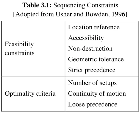
The task of operation sequencing is complicated by the large number of interactions that exist between the various factors which affect decision-making. According to Usher and Bowden [8], the factors which are resource independent shown inTable 3.1. The constraints which affect sequencing can be divided into those which address either the feasibility or optimality of a sequence. This division permits the construction of a system which applies the feasibility constraints to the task of generating alternative sequences, and the optimality criteria to the task of judging the quality of the resulting alternatives. A feasible sequence is one which does not violate any of the feasibility constraints listed in Table. 3.1.
Table 3.1: Sequencing Constraints [Adopted from Usher and Bowden, 1996]
Feasibility constraints
Location reference Accessibility Non-destruction Geometric tolerance Strict precedence
Optimality criteria
Number of setups Continuity of motion Loose precedence
In this research, we only consider feasibility constraints, because the optimality criteria will be considered in another stage. The feasibility constraints adopted here is shown in Table 3.2.
Table 3.2: New Sequencing Constraints
Feasibility constraints
The location constraint is concerned with an examination of the defined part features to determine what reference face is used to locate each feature. This reference identifies the necessity that the locating surface be machined prior to the associated feature. In order to machine a feature it must be accessible. The accessibility constraint evaluates each feature's accessibility based on the feature type and its location relative to other features. Features are defined as either primary or secondary. The primary features define the basic shape of the part (diameters, tapers, etc) and secondary features provide the detailed shape aspects (grooves, bends, etc.). The fact that a secondary feature is defined as residing on a primary feature, it makes sense not to machine the secondary feature until the primary feature has been formed. Therefore, before a secondary feature, such as a groove, is cut on the taper of the part, the taper (a primary feature) must be machined to specifications.
3.5 Operation Sequence Coding
Application of an evolutionary search technique like genetic algorithms (GA) requires a method for representing a solution. An obvious choice would be to represent a sequence as a string whose elements define a list of operations, or possibly the features processed by those operations. However, inherent within this representation is the need to express the constraints which must be fulfilled by the resulting sequence. Therefore, most representations begin from this point, adding attributes to the definition of each element in the string or devising a method of coding the representation to impose these constraints.
Since operation sequencing problem is an order-based problem like travel salesman problem, we used path representation to represent the sequence. In this problem a sequence is represented as a list of n operations. If operation ‘i’ is the j-th element of the list, operation ‘i’ is the j-th operation to be performed. Hence, the sequence 3-2-5-6-1-4 is simple represented by 325614.
Then, we used a sequence of operations as the chromosome structure. Each chromosome is a sequence of operations to be performed, in order to produce a part, as follows:
The sequence of operations is bounded to the precedence constraints. Table 3.3 shows the example of precedence constraints for a number of processes. O04,…, O07 is a set of flexible-route operations which can be performed in any order.
Table 3.3: Precedence constraints
Id Operation Precedes
O1 Shearing O2
O2 Center Hole Punching O3, O4 ,O5 ,O6 ,O7
O3 Berlin Eye Forming nil
O4 Short tapering O5 ,O6 ,O7 O5 End punching O4 ,O6 ,O7 O6 Bevel hole punch O4 ,O5 ,O7 O7 Diamond cut O4 ,O5 ,O6
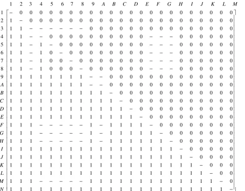
There are several approaches have been used to represent precedence relationships among features. They are feature precedence graph (FPG) [8], rules [3] and precedence relationship matrix (PRM) [6]. In this research, we used another kind of precedence-relation matrix as shown in Figure 3.1 to represents the constraints and relationships between the operations.
Figure 3.1: Precedence-Relation Matrix
1 2 3 4 5 6 7 8 9
1 0 0 0 0 0 0 0 0 0 0 0 0 0 0 0 0 0 0 0 0 0 0 2 1 0 0 0 0 0 0 0 0 0 0 0 0 0 0 0 0 0 0 0 0 0
3 1 1 0 0 0 0 0 0 0 0 0 0 0 0 0 0 0
4 1 1 0 0 0 0 0 0 0 0 0 0 0 0 0 0 0 0
5 1 1 1 0 0 0 0 0 0 0 0 0 0 0 0 0 0 0
6 1 1 1 0 0 0 0 0 0 0 0 0 0 0 0 0 0 0
7 1 1 1 0 0 0 0 0 0 0 0 0
8 9
A B C D E F G H I J K L M N
A B C D E F G H I J K L M N − − − − − − − − − − − − − − − − − − − − − − −
− − − − 0 0 0 0 0 0
1 1 1 0 0 0 0 0 0 0 0 0 0 0 0 0 0 0
1 1 1 1 1 1 1 1 0 0 0 0 0 0 0 0 0 0 0 0 0
1 1 1 1 1 1 1 1 0 0 0 0 0 0 0 0 0 0 0 0 0
1 1 1 1 1 1 1 1 1 1 0 0 0 0 0 0 0 0 0 0 0 0 1 1 1 1 1 1 1 1 1 1 1 0 0 0 0 0 0 0 0 0 0 0 1 1 1 1 1 1 1 1 1 1 1 1 0 0 0 0 0 0 0 0 0 0 1 1 1 1 1 1 1 1 1 1 1 1 1 0 0 0 0 0 0 0 0 0
1 1 1 1 1 1 1 1 0 0 0 0 0 0 0 0
1 1 1 1
− − − − − − − − − − − − − − − − − − − − −
− − − − − 1 1 1 1 1 0 0 0 0 0 0 0
1 1 1 1 1 1 1 1 1 1 0 0 0 0 0 0
1 1 1 1 1 1 1 1 1 1 1 1 1 1 1 1 1 0 0 0 0 0 1 1 1 1 1 1 1 1 1 1 1 1 1 1 1 1 1 1 0 0 0 0 1 1 1 1 1 1 1 1 1 1 1 1 1 1 1 1 1 1 1 0 0 0 1 1 1 1 1 1 1 1 1 1 1 1 1 1 1 1 1 1 1 1 0 0
1 1 1 1 1 1 1 1 1 1 1 1 1 1 1 1 0
1 1 1 1 1 1 1 1 1 1 1 1 1 1 1 1 1 1 1 1 1 1
The value of the matrix is either
if can precede
if can not precede
if and are two alternative operations
0 1 ij i j i j i j ρ = −
3.6 Fitness Function
For our problem, the fitness of a chromosome is obtained by computing the cost of penalty for the constraints violation according to the sequence of the chromosome. Thus our objective function is to
subject to the precedence constraints represented by precedence-relation matrix (PRM) shown in Figure 3.1.
3.7 GA Operators
There are usually three operators in a typical genetic algorithm [11]. The first is the reproduction operator which makes one or more copies of a well performing individual compared to the rest of individuals in the population; otherwise, the individual is eliminated from the solution pool. For example, consider two individuals. The first individual is considered to perform better than the second one. After the reproduction operator is applied, the first individual is duplicated; the second individual is eliminated from the population, due to its low performance.
The second operator is the mutation operator. This operator acts as a background operator and is used to explore some of the unvisited points in the search space by randomly flipping a bit in a population of strings. During the past decade, several mutation operators have been proposed
1
1 1
min
n n
ij
i j i
i, j in the sequence
p −
= = +
∀
for permutation representation, such as inversion, insertion, displacement, and reciprocal exchange mutation.
The third operator is the recombination (also known as the crossover) operator. This operator selects two individuals within the generation and a crossover site and performs a swapping operation of the string bits to the right hand side of the crossover site of both individuals. The outcome of the crossover operation is two individuals that possess some traits inherited from both parents. In this research, in order to guarantees that the resulting offspring is a legal sequence, we used two methods of path representation for mutation and crossover.
3.8 Mutation
There are number of crossover operators and mutation operators that can be applied with path representation in order to solve this problem.
For mutation we used reciprocal exchange method which swaps two values in the individual. The algorithms will randomly choose two mutation points and swap the values in those particular points.
As shown in Figure 3.2, reciprocal exchange mutation selects two positions at random and swaps the values on these positions.
Figure 3.2: Mutation using Reciprocal Exchange Parent 1
Offspring 1
8 A 2 E J D B 4 C 1
8 A 2 4 J D B E C 1 Two mutation points randomly
chosen
3.9 Crossover
There are three crossovers were defined for the path representation: partially-mapped (PMX) [12], order (OX) [13] and cycle (CX) [14] crossovers.
Figure 3.3: Order-based or cyclic crossover
The crossover used in this algorithm is a version of the order crossover (OX) which also known in [15] as cyclic crossover. As revealed in Figure 3.4, two parents (with a random cut point marked by | ) would produce the offspring in the following way. First, the segments before cut point are copied into offspring. Next the values from the other parent are copied in the same order from the beginning of the string, omitting symbols already present.
3.10 Multi-population Directed Genetic Algorithms
In order to accelerate the performance of GA, we introduce two types of accelerators. The goal of the first accelerator is to terminate the evolution when the optimal solution found. In this
6 I 2 E J D B 4 C 1
I C 2 4 1 5 B E D 9
5 9
J 6
Parent Parent
Parent2
Parent1 Offspring
Offspring2
I C 2 4 1 5 B E D 9 6 J
D C 2 4 1 5 B I E J 6 9
6 I 2 E J D B 4 C 1 9 5
case, the optimal solution found if all the precedence constraints is satisfied. If this is the case, the GA stops their iteration and return current population as an optimal solution.
Figure 3.4: Directed Mutation
On the other hand, the second accelerator is used to accelerate the individuals move towards the optimal solutions. When the solution in the population did not show any improvement, GA will force for improvement using directed mutation. Using this directed mutation, the algorithms randomly pick one individual and force the mutation for any unsatisfied values.
As shown in Figure 3.5, feasibility of each two consecutive values in the selected individual will be checked and which are not satisfying the precedence constraints will be swapped.
In addition, we used multi-population genetic algorithms topology to enable a number of parts’ sequence from a single product being sequenced in a single run. The number of parts n extracted from product design and being used to produce the number of population. As shown in Figure 3.5, n number of populations have to go through the same processes namely, reproduction, mutation and crossover, then will produce their own optimal solution.
J 1 2 4 8 A C B D E
J 1 2 4 8 A B C D E
The feasibility of each two consecutive values will be checked and which are not satisfied
will be force to be satisfied
Figure 3.5: Multi-population GA
3.11 Results and Discussion
The goal of sequencing is to find an operation sequence which satisfies the constraints mentioned in the previous section. The constraints have been representing in the form of precedence-relation matrix (PRM).
In order to demonstrate the practicability and efficiency of the proposed algorithm, different numerical simulations are tested and evaluated. The algorithm is run on a personal computer with an Intel Pentium IV, 512MB RAM, on Microsoft Windows 2000 Professional. The codes are written in the LISP language.
Each trial run of our program started with a randomly created generation of individuals. The program was allowed to evolve this generation up to 50 times.
In order to show the effectiveness of the proposed algorithms, several runs have been done to be compared with the result from standard genetic algorithms (SGA).
solution part
population 1 … population
n
mutation
crossover reproductio
mutation
crossover reproduction
solution part
n solutions
n populations
Multi-population GA
Figure 3.6: Modified PSO vs Standard GA (Run 1)
Figure 3.6 show the comparison results for Modified PSO vs Standard Genetic Algorithms (SGA). The graphs show that in each trial modified PSO found the solution earlier than SGA.
Figure 3.7: Modified PSO vs Standard GA (Run 2)
Figure 3.8: Modified PSO vs Standard GA (Run 3)
This is of the most significant advantage for PSO compared to GA. With a number of candidate solutions PSO can come out with a near optimal solution faster than GA. However, the author believes that GA also can perform this advantage through parallel structure. Hence, we conclude that the performance of PSO is comparable with parallel GA.
3.12 Conclusion
The results show that the implementation of multi-population GA enables us to optimize a number of parts (sequences) for a single product using a single run. This can increase the efficiency of the algorithms because we no need to have a multiple run of GA for a single product.
On the other hand, directed GA is used to accelerate the individuals move toward the optimal solutions. This can help us to get the solution without a long waiting time.
3.13 Acknowledgements