Classification and Variable Selection Methods for Ultrahigh Dimensional and Imbalanced Data.

ABSTRACT

LIU, ZHONGKAI. Classification and Variable Selection Methods for Ultrahigh Dimensional and Imbalanced Data. (Under the direction of Howard D. Bondell.)

Classification and variable selection play important roles in machine learning and sta-tistical applications. Classification methods are used in a broad range of application areas, from medical diagnosis to anomaly detection in signal analysis, from credit risk screening to quality control, from image segmentation to information retrieval. Variable selection or feature selection, whose purpose is to eliminate irrelevant variables, is undoubtedly important, especially in high dimensional applications.

Although there are a large number of classification and variable selection methods so far, classification and variable selection on imbalanced data, i.e. a large skew in the class distribution, is a challenging problem. Evaluation of classifiers via the receiver operating characteristic (ROC) curve is common in binary classification. Techniques to develop classifiers that optimize the area under the ROC curve have been proposed. However, for imbalanced data, the ROC curve tends to give an overly optimistic view. Realizing its disadvantages of dealing with imbalanced data, Precision-Recall (PR) curves have recently become a basis for assessing classification methods on class-imbalanced data.

In this thesis work, we focus on classification and variable selection methods for ultrahigh dimensional and imbalanced data. Specifically, we investigate two types of problems. The first problem is related to the imbalanced data sets, i.e. there are many more examples from some classes than from others. The imbalanced problem is prevalent in many applications, including fraud and churn detection, text categorization, medical diagnosis, detection of software defects, etc. The second problem is on ultrahigh dimensions, where the dimension of variables is much larger than the sample size. Due to the huge improvement in data gathering and data processing mechanisms, ultrahigh dimensional data arises in various areas of modern scientific research using quantitative measurements.

© Copyright 2016 by Zhongkai Liu

Classification and Variable Selection Methods for Ultrahigh Dimensional and Imbalanced Data

by Zhongkai Liu

A dissertation submitted to the Graduate Faculty of North Carolina State University

in partial fulfillment of the requirements for the Degree of

Doctor of Philosophy

Statistics

Raleigh, North Carolina

2016

APPROVED BY:

Tao Pang Peter Bloomfield

Rui Song Howard D. Bondell

DEDICATION

BIOGRAPHY

ACKNOWLEDGEMENTS

I would like to thank my advisor and Director of Statistics Graduate Programs, Dr. Howard Bondell, for his insightful guidance and constant help for my study and research. As an expert in variable selection and classification methods, he is connecting the academic research with the industry world closely, which grows my passion for statistics and research. The weekly meetings with him over 3 years bring me the inspiration and open my horizon not only in the PhD research but in my career development as well. I feel lucky to have such an excellent professor as my advisor.

I would also like to extend my appreciation to Dr. Rui Song, Dr. Tao Pang, and Dr. Peter Bloomfield, for their selfless encouragement and valuable mentorship. Admittedly, Dr. Rui Song is my first research mentor who initiates me into the statistics research. I sincerely express my gratitude to her for the generous guidance and considerate patience during our project on high dimensional data analysis, which is a great start in my PhD career. I regard Dr. Tao Pang as a lifelong mentor who shows me the magic of quantitative analysis in the financial market. Talking with him is thought-provoking, leading to fruitful remarkable work including our published paper An Efficient Grid Lattice Algorithm for Pricing American-style Options onInternational Journal of Financial Markets and Derivatives and more smart ideas about risk management in progress. I really appreciate the precious quantitative research work with him. Dr. Peter Bloomfield is my professional mentor on a business analytical project in Allegro MicroSystems, where I completed my first internship. I have learned a lot form his intelligence and diligence throughout the project, not only on predictive modeling and time series analysis skills, but also the passion and strictness for the truth. It is my great honor to have you all in my PhD committee.

Daowen Zhang, the experimental statistics course by Dr. Jason Osborne, and so on, play significant parts in my statistician career. All the training helps me get the challenging data science internship in AT&T Big Data Team in Silicon Valley during the summer of 2015, a great opportunity to work with the smartest engineers and inspire my deeper enthusiasm about data science.

TABLE OF CONTENTS

LIST OF TABLES . . . viii

LIST OF FIGURES . . . ix

Chapter 1 Introduction . . . 1

Chapter 2 Optimal Classification of Imbalanced Data . . . 5

2.1 Introduction . . . 5

2.2 ROC and Precision-Recall curves . . . 7

2.2.1 Preliminaries . . . 7

2.2.2 Binormal assumption . . . 7

2.2.3 ROC curve . . . 8

2.2.4 Precision-Recall curve . . . 9

2.3 Estimators and asymptotic properties . . . 11

2.3.1 ROC curve . . . 12

2.3.2 Precision-Recall curve . . . 13

2.4 Simulation . . . 15

2.4.1 Simulation Model I . . . 15

2.4.2 Simulation Model II . . . 16

2.4.3 Simulation Model III . . . 19

2.5 Real data analysis . . . 20

2.6 Discussions . . . 21

Chapter 3 Feature Selection for Imbalanced Data . . . 23

3.1 Introduction . . . 23

3.2 Regularized Binormal Precision-Recall Algorithm . . . 24

3.2.1 Anchor Variable . . . 25

3.2.2 Threshold Gradient Descent Regularization (TGDR) . . . 25

3.2.3 Regularized Binormal Precision-Recall Algorithm . . . 26

3.3 Simulation . . . 27

3.3.1 Simulation Model I . . . 28

3.3.2 Simulation Model II . . . 29

3.4 Real Data Analysis . . . 35

3.5 Discussions . . . 38

Chapter 4 Variable Screening in Ultrahigh Dimensions . . . 41

4.1 Introduction . . . 41

4.2 Generalized linear models . . . 43

4.3 Principal component analysis . . . 43

4.4.1 PCAS with maximum marginal likelihood estimators . . . 45

4.4.2 PCAS with marginal likelihood ratio . . . 46

4.4.3 Determining the number of selected variables . . . 47

4.4.4 Determining the number of principal components . . . 47

4.5 Simulations . . . 47

4.5.1 Simulation Model I . . . 48

4.5.2 Simulation Model II . . . 49

4.5.3 Simulation Model III . . . 51

4.5.4 Simulation Model IV . . . 54

4.6 Real data analysis . . . 56

4.6.1 Affymetric GeneChip Rat Genome 230 2.0 Array Example . . . . 56

4.6.2 European American SNP Example . . . 58

4.7 Discussions . . . 59

References . . . 60

Appendices . . . 71

Appendix A Proof of Proposition 2 . . . 72

LIST OF TABLES

Table 2.1 Confusion Matrix. . . 7 Table 2.2 Estimates of the risk score function by PR and ROC methods under

simulation Model I. . . 16 Table 2.3 Comparison between asymptotic and sample variance of PR estimate

under simulation Model I. . . 16 Table 2.4 Estimates of the risk score function by PR and ROC methods under

simulation Model II. . . 18 Table 2.5 Comparison in the area under the PR and ROC curve among different

classifiers. . . 19 Table 2.6 Characteristics of datasets. . . 21

Table 3.1 Characteristics of Abalone9 18 data set. . . 35

Table 4.1 The MMMS and RSD (in parenthesis) of the simulated examples for linear and logistic regression from simulation model I with n = 500 when p= 1000 and p= 10000. PC=0 refers to the marginal screening in Fan and Lv (2008). . . 50 Table 4.2 The MMMS and RSD (in parenthesis) of the simulated examples for

linear and logistic regression model II using different number of PCs with n= 500 when p= 1000 andp= 10000. . . 52 Table 4.3 The MMMS and RSD (in parenthesis) of the simulated examples for

linear and logistic regression model III using different number of PCs with n= 500 when p= 1000 andp= 10000. . . 53 Table 4.4 The MMMS and RSD (in parenthesis) of the simulated examples for

LIST OF FIGURES

Figure 2.1 The difference between comparing algorithms in ROC vs PR space. . 10 Figure 2.2 Scatter plot of the example dataset with PR and ROC linear classifiers

under simulation Model II. . . 17 Figure 2.3 False discovery rate by PR and ROC methods under simulation Model II. 18 Figure 2.4 False discovery rate by PR and ROC methods under simulation Model

III. . . 20 Figure 2.5 Relationship between average false discovery rate and true positive

examples. . . 22

Figure 3.1 False discovery rate by PR and ROC methods under simulation Model I. 30 Figure 3.2 False positive rate by PR and ROC methods under simulation Model I. 31 Figure 3.3 False discovery rate by PR and ROC methods under simulation Model II. 33 Figure 3.4 False positive rate by PR and ROC methods under simulation Model II. 34 Figure 3.5 False discovery rate by regularized binormal PR and ROC methods

under Abalone9 18 real data. . . 36 Figure 3.6 False positive rate by regularized binormal PR and ROC methods

under Abalone9 18 real data. . . 37 Figure 3.7 False discovery rate difference between PR and ROC methods under

Abalone9 18 real data. . . 39 Figure 3.8 False positive rate difference between PR and ROC methods under

Abalone9 18 real data. . . 40

Figure 4.1 The Scree Plot for Linear Models in Simulation Model I with p= 1000 and n= 500. . . 49 Figure 4.2 The Scree Plot for Linear Models in Simulation Model II withp= 1000

and n= 500. . . 51 Figure 4.3 The Scree Plot for Linear Models in Simulation Model III withp= 1000

and n= 500. . . 54 Figure 4.4 Scree Plot for Linear Models in Simulation Model IV with p= 40000

CHAPTER

1

Introduction

Classification and variable selection are hot topics in machine learning and statistical applications. Classification methods solve the problem of identifying to which of a set of categories a new observation belongs, based on a training set of data containing observations whose category membership is already known, in a broad range of application areas, from medical diagnosis to anomaly detection in signal analysis, from credit risk screening to quality control, from image segmentation to information retrieval. Feature or variable selection is to eliminate irrelevant variables to enhance the generalization performance of a given learning algorithm, especially in high dimensional applications. In regression and classification problems with a large number of predictors, if only some of the variables contribute to the response, overfitting appears to be a critical concern for statistical analysis. Consequently, finding the optimal subset of variables among the pool is necessary and momentous.

and McNeil, 1982) appeared as a graphical plot that illustrates the performance of a binary classifier system as its decision threshold is varied. However, Davis and Goadrich (2006) pointed out the disadvantage of ROC curves whenever there is a large skew in the class distribution. In terms of classification of highly imbalanced data, ROC curves tend to present an overly optimistic view of an algorithm’s performance. In fact, there are many situations where a large skew exists, such as anomaly detection for rare events. As an alternative to ROC curves for tasks with imbalanced data, Precision-Recall (PR) curves (Raghavan et al., 1989) have recently become a basis for assessing classification methods.

Davis and Goadrich (2006) discussed the relationship between ROC and Precision-Recall curves, and Craven (2005); Davis et al. (2005); Kok and Domingos (2005); Singla and Domingos (2005) cited Precision-Recall curves as a better tool considering its performance in front of imbalanced data.

controlling the search for local interactions and employing more effective variable and split selection strategies. Loh (2012) presented an alternative method, derived from the GUIDE classification and regression tree algorithm, that employs recursive partitioning to determine the degree of importance of the variables. Recently Tang et al. (2014) proposed a nonparametric method for variable selection and classification called Categorical Adaptive Tube Covariate Hunting (CATCH) that constructs a nonparametric measure of the relational strength between each predictor and the categorical response, and retains those predictors whose relationship to the response is above a certain threshold. The second group includes methods that incorporate variable selection by applying shrinkage methods with norm constraints (Frank and Friedman, 1993) on the parameters that generate sparse vectors of parameter estimates. Bradley and Mangasarian (1998) investigated the use of

L1 penalty (Tibshirani, 1996) in the support vector machine (SVM) (Vapnik and Vapnik,

1998) to do the variable selection. Zhu et al. (2004) proposed an algorithm for calculating the solution path of the L1 SVM as a function of its tuning parameter. Wang and Shen

(2007); Zhang et al. (2008) implemented variable selection with classification based on SVM, and Qiao et al. (2008) incorporated variable selection into linear discriminant analysis (Fisher, 1936; McLachlan, 2004). Liu and Wu (2012) designed a SVM-based variable selection method in regression and classification via a new penalty that combines the L0 and L1 penalties.

gradient descent regularization method (Friedman and Popescu, 2003) to maximize the area under the Precision-Recall curve.

Another problem we consider is ultrahigh dimensions, where the dimension of variables is much larger than the sample size. Due to the huge improvement in data gathering and data processing mechanisms, ultrahigh dimensional data arises in various areas of modern scientific research using quantitative measurements. However, it is often the case that only a relatively small subset of the predictors contribute to the response. Considering the computation cost, statistical accuracy and robustness in the ultrahigh dimensional problem, lots of traditional statistical methods fail to work, including bridge regression (Frank and Friedman, 1993), LASSO (Tibshirani, 1996), SCAD (Fan and Li, 2001), Dantzig selection (Candes and Tao, 2007), and other folded concave regularization methods (Fan and Lv, 2011; Zhang and Zhang, 2012). In this thesis work, we propose a principal component-adjusted screening (PCAS) method for generalized linear models, which uses principal components as surrogate covariates to account for omitted covariates in marginal screening.

CHAPTER

2

Optimal Classification of Imbalanced Data

2.1

Introduction

Consider a classification problem with n independent observations. Denote the observed data by {(Xi, Yi), i= 1,· · · , n} with Xi ∈ Rp andYi ∈ {0,1}. We consider the linear risk score as our basis for classification so that we classify toY = 1 if βTX> cbased on some decision threshold c. Note that any monotone transformation ofβTX can be applied, so this is essentially a single index model.

Assuming classification based on the linear risk score, the task is to estimateβ. Methods based on misclassification rate or surrogates, such as support vector machines (SVMs) (Cortes and Vapnik, 1995), rely on a fixed threshold that is estimated as an intercept. Since the overall performance of a classifier can be measured by the area under the curve (AUC), either ROC or PR curve, β can be estimated by maximizing the AUC value.

Pan, 1999; Pepe, 2003), which assumes a pair of normal distributions underlying the positive and negative groups. Pepe (2003) showed that the binormal AUCROC provides more valuable information and exhibits more stability than the empirical AUC in the low dimensional situation, while in the high dimensional case the binormal AUCROC is computationally more affordable than the empirical one. Ma et al. (2006) implemented the threshold gradient descent regularization method for estimation and selection with the binormal AUCROC as the objective function.

On the other hand, an empirical Precision-Recall curve is difficult to use because of its sensitivity to idiosyncracies in the data, especially at high precisions (Davis and Goadrich, 2006). Cl´emen¸con and Vayatis (2009) addressed this problem by applying a nonparametric approach to derive a smooth Precision-Recall curve. Boyd et al. (2013) gave a detailed overview of current methods to compute the area under the empirical Precision-Recall curve, including lower trapezoid, average precision, interpolated median, and confidence interval estimation. In order to overcome the disadvantages of the empirical version, Brodersen et al. (2010b) discussed the Precision-Recall curve on the basis of the binormal model.

Although discussion of the Precision-Recall curve appears in the literature, its usage has been solely for evaluation of computing classifiers. However, given that it is recommended to evaluate classifiers, it seems natural to use this criterion to estimate the classifier directly. This is what is proposed in this thesis work. We propose an approach for binary classification with imbalanced data in a binormal framework. The approach is to estimate the risk score function via maximization of the area under the Precision-Recall curve based on the binormal assumption. We demonstrate via both theoretical arguments, as well as simulation and real data, that the proposed approach outperforms approaches based on the area under the ROC curve.

2.2

ROC and Precision-Recall curves

2.2.1

Preliminaries

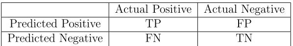
A confusion matrix is a structure that represents the binary classification result for a particular choice of threshold, c, as shown in Table 2.1. We follow the notations in Davis and Goadrich (2006). We call Y = 1 a positive example, and Y = 0 a negative example. True Positives (TP) represent examples correctly labeled as positive, while False Positives (FP) represent negative examples but labeled incorrectly as positive. True Negatives (TN) refer to negative examples that are correctly labeled as negative. Similarly, False Negatives (FN) correspond to those indeed positive while labeled as negative examples. Based on the confusion matrix, as a function of the threshold, we can construct an ROC curve or a Precision-Recall curve. Furthermore, based on the binormal assumption, it becomes a parametric confusion matrix, and a functional form of the ROC curve and Precision-Recall curve can be derived. As a result, the area under the curve, including AUCROC and AUCPR, can be computed.

Table 2.1: Confusion Matrix.

Actual Positive Actual Negative

Predicted Positive TP FP

Predicted Negative FN TN

2.2.2

Binormal assumption

For a given threshold c, we classify to Y = 1 if the decision score βTX> c, andY = 0 otherwise. Dorfman and Alf (1968); Brodersen et al. (2010b) described the binormal assumption, which is to assume the decision scores to follow two independent Gaussian distributions, one for the positive group and one for the negative group expressed as

βTX|Y = 1∼Normal(µp, σ2p),

where without loss of generality, assume µp ≥µn. If not, we can change the sign ofβ. Zou and Hall (2000); Krzanowski and Hand (2009) displayed broad applications of the binormal assumption. Note that the normality assumption is on a linear combination of X rather thanX itself. This assumption on a linear combination would be more likely to hold, particularly for moderate to large p, due to the Central Limit Theorem effect.

2.2.3

ROC curve

The ROC curve plots the true positive rate (TPR) against the false positive rate (FPR), where FPR and TPR are computed based on the information from the confusion matrix.

TPR = T P

T P +F N,

FPR = F P

F P +T N.

Based on the binormal assumption it follows that

TPR =P(βTX> c|Y = 1) = 1−Φ

c−µp

σp

, (2.1)

FPR =P(βTX> c|Y = 0) = 1−Φ

c−µn

σn

. (2.2)

After some algebra, the relationship betweeen TPR and FPR, i.e. the ROC curve by (FPR, TPR) pairs is of the form:

TPR = Φ

µp−µn

σp

+ σn

σp

Φ−1(FPR)

, (2.3)

linear classifier, the area under ROC curve can be equivalently represented as

AUCROC = P(βTXp >βTXn) =P(βTXp−βTXn >0)

= 1−Φ −_pµp −µn

σ2

p +σ2n

!

= Φ _pµp−µn

σ2

p +σ2n

!

, (2.4)

where Xp denotes a random draw from the distributionX|Y = 1 and Xn, a random draw from the distributionX|Y = 0.

2.2.4

Precision-Recall curve

Precision-Recall curves instead plot Precision, measuring the fraction of examples classified as positive that are truly positive, versus Recall (same as TPR). The key difference is in the use of Precision instead of FPR. This is akin to the use of False Discovery Rate instead of Type I error in multiple testing problems. Unlike the ROC curve, the Precision-Recall curve will also depend on the fraction of positive examples, denoted as π. Based on the confusion matrix, binormal assumption and linear classifier, Recall and Precision can be expressed as

Recall = TPR = T P

T P +F N =P(β

T_{X> c|Y = 1) = 1−Φ(}c−µp

σp ),

Precision = T P

T P +F P =P(Y = 1|β

T_{X> c)}

= P(β

T

X> c|Y = 1)P(Y = 1)

P(βTX> c|Y = 1)P(Y = 1) +P(βTX> c|Y = 0)P(Y = 0) (By Bayes’ Rule)

= π×Recall

π×Recall + (1−π)[1−Φ(c−µn

σn )]

.

By linking Recall and Precision through the threshold c, the relationship between Precision and Recall, i.e. the Precision-Recall curve, can be expressed as

Precision = π×Recall

π×Recall + (1−π)Φ(µn−µp

σn +

σp

σnΦ

The area under the Precision-Recall curve is then

AUCPR =

Z 1

0

π×t π×t+ (1−π)Φ(µn−µp

σn +

σp

σnΦ

−1_(t))dt, (2.6)

where t= Recall.

The PR space has a clear advantage over the ROC space when facing imbalanced data, and this difference exists because in this domain the number of negative examples greatly exceeds the number of positive examples. Consequently, a large change in the number of False Positives can lead to a small change in the false positive rate used in ROC analysis. Precision, on the other hand, by comparing False Positives to True Positives rather than the total number of negative examples, captures the effect of the large number of negative examples on the algorithm’s performance.

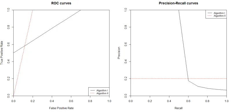
Consider two competing algorithms for classification on an imbalanced data set with 100 positive examples and 2000 negative examples. Figure 2.1 shows the performance of each algorithm in ROC and PR space.

Figure 2.1: The difference between comparing algorithms in ROC vs PR space.

not perform well in terms of false discovery rate. The false discovery rate (FDR) is the proportion of false discovered positives among the total number of predicted positives, which is defined in Equation (2.7) based on Table 2.1.

FDR = F P

T P +F P. (2.7)

Consider, for example, the first time each algorithm is able to select 50 out of the 100 positive examples, i.e. the first time each curve reaches a height of TPR=0.5 on the left panel of Figure 2.1. For algorithm II, this occurs at the point (0.1,0.5), i.e. 200 false positives and 50 true positives, algorithm II gives a high false discovery rate of 200/(200 + 50) = 0.8. On the other hand, algorithm I can achieve the same level of true positive rate (0.5) without making any false positives, leading to zero false discovery rate. In practice, in most typical cases, we prefer algorithm I although it has a comparatively smaller AUCROC. The reason for this is the large amount of area that includes regions of high false positive rate. Unlike the ROC space, the PR space suggests to choose algorithm I based on its larger AUCPR (0.598) compared to algorithm II (0.2). Consequently, in terms of classifying the imbalanced data, ROC curves tend to present an overly optimistic view of an algorithm’s performance, while Precison-Recall curves give a more appropriate picture.

2.3

Estimators and asymptotic properties

For j = 0,1, we denoteµ_j = E(X|Y =j) and Σj = Var(X|Y =j). We assume that µ0, µ₁, Σ0 and Σ1 exist, and at least one of {Σ0,Σ1} is non-singular. The goal is to find

2.3.1

ROC curve

According to the binormal assumption and Equation (2.4),

AUCROC = Φ





βT(µ₁−µ₀)

q

βT(Σ1+ Σ0)β 

. (2.8)

Due to the monotonicity of the cumulative distribution function, Φ(·), the maximizer of

βT

(µ₁−µ₀)

q

βT(Σ1+Σ0)β

will maximize the AUCROC. Finally, we may solve the equivalent problem

max

β∈Rp

βT(µ₁−µ₀)(µ₁−µ₀)T_β

βT

(Σ1+Σ0)β

subject to βT(µ₁ −µ₀)≥0.

Proposition 1. For symmetric matrix A, the solution to the problem max x∈Rn

xT_{Ax subject} to xTx= 1 will be the eigenvector for the largest eigenvalue of A, and the maximum value ofxTAx is the largest eigenvalue. In particular, any vector which is proportional to the eigenvector for the largest eigenvalue of A will maximize x_xTTAx_x .

Let γ = (Σ1+ Σ0)1/2β, then

βT(µ₁−µ₀)(µ₁−µ₀)T_β

βT(Σ1+ Σ0)β

= γ T_(Σ

1+ Σ0)−1/2(µ1−µ0)(µ1−µ0)T(Σ1+ Σ0)−1/2γ

γT_γ .(2.9)

Note that, since both Σ0 and Σ1, are negative definite and at least one is

non-singular, it follows that Σ1+Σ0is positive definite. By Proposition 1, a solution to (2.9) will

be proportional to the first eigenvector of (Σ1+ Σ0)−1/2(µ1−µ0)(µ1−µ0)T(Σ1+ Σ0)−1/2

and thus, since this is a rank one matrix, it follows that γ ∝ (Σ1 + Σ0)−1/2(µ1−µ0).

Consequently,

β ∝(Σ1+ Σ0)−1(µ1−µ0). (2.10)

Let _Sj = {i : Yi = j}, j = {0,1} be the index set to distinguish the positive and negative group, and letnj =|Sj|. The sample version of Equation (2.10) will be

ˆ

β= (S1+S0)−1( ¯X1−X¯0), (2.11)

where S1 and ¯X1 are the sample variance and mean for predictors in the positive group,

2.3.2

Precision-Recall curve

Area under the Precision-Recall curve

According to the binormal assumption and Equation (2.6),

AUCPR =

Z

0

πt

πt+ (1−π)Φ

βT(µ₀−µ₁)

q

βTΣ0β

+ q

βT

Σ1βΦ−1(t)

q

βTΣ0β

dt. (2.12)

Since there is no closed form solution to Equation (2.12), we can solve it numerically via algorithms such as gradient descent, which is the approach that we implement in the examples.

In practice, (µ₀,µ₁,Σ0,Σ1) is again replaced by its sample counterpart ( ¯X0,X¯1, S0, S1).

Asymptotic distribution of the estimator

For simplicity of presentation, we consider the bivariate case here. For j = 0,1, let E(X|Y =j) =µ_j = (µj1, µj2)T, and

Var(X|Y =j) = Σj =

σ2

j1 cj

cj σj22 !

,

where cj denotes the covariance betweenX1 andX2 given Y =j. To create identifiability

in β, we fix |β1| = 1. The goal is to estimate the linear score function in the form of

bX1+βX2 (b∈ {−1,1}) which maximizes the area under the Precision-Recall curve. The

population version of the problem can be described as

(b0, β0) = argmax

b∈{−1,1},β∈R Z 1

0

πt

πt+(1−π)Φ(µn_σn−µp+σp_σnΦ−1_(t))dt, s.t. (2.13)

µp =bµ11+βµ12, µn =bµ01+βµ02,

σ2

p =σ112 +β2σ122 + 2bβc1, σn2 =σ201+β2σ202+ 2bβc0.

Proposition 2. Under the binormal assumption, the solution, or population parameter, (b0, β0), that maximizes the area under the Precision-Recall curve satisfies

where the functions, λj0 = λj(b0, β0, µp0, µn0, σp0, σn0) for j = 1,· · · ,4 are given in the

Appendix A, with µp0 =b0µ11+β0µ12, and µn0, σp0, σn0 are defined similarly.

The proof of proposition 2 is also given in the Appendix A.

Assume that X|Y = j follows a bivariate normal distribution with mean µ_j and variance Σj forj = 0,1. By applying Neyman-Pearson (NP) theory to binary hypothesis testing, we can reach an optimal risk score function by finding the most powerful test. Specifically, the null hypothesis is that the example belongs to the positive group, while the alternative hypothesis sets the example to the negative group. By NP theorem as well as the bivariate normal distribution setting, we will assign an example with observed X

to the positive group if

(2π)−1_|Σ

1|−1/2exp(−(X−µ1) 0

Σ−₁1(X−µ₁)) (2π)−1_|Σ

0|−1/2exp(−(X−µ0) 0

Σ−₀1(X−µ₀)) > η0 =⇒(X−µ₀)0Σ−₀1(X−µ₀)−(X−µ₁)0Σ₁−1(X−µ₁)> η1

=⇒X0(Σ−₀1−Σ−₁1)X+ 2(Σ₁−1µ₁−Σ−₀1µ₀)0X> η, (2.15)

where η0, η1, and η are all constants.

If assuming equal covariance matrices, i.e. Σ0 = Σ1 = Σ, then the optimal score

function, which is the left hand side of (2.15), will be linear withβ? ∝Σ−1_(µ

1−µ0). It

can be shown that any (b0, β0)∝β? is also the unique set of solutions to (A.4). Hence

the sample version of (A.1) will be a consistent estimator for the optimal classifier. The estimator using the AUCROC, will also converge to the same quantity. Otherwise, for nonequal covariance matrix, the optimal score will be quadratic. In this case, or the case of non-normality, the true β0 will satisfy Equation (A.4). In that situation, the maximizer

for AUCROC will differ from that of AUCPR.

If the predictors are conditionally independent within each group, i.e. c1 = c0 = 0,

then Equation (A.4) becomes

λ10µ12+λ20µ02+ 2λ30β0σ122 + 2λ40β0σ202= 0. (2.16)

of the covariance matrix in the positive group and that in the negative group are the same, we can simply transform to the principal components as our predictors to build the classifier.

Theorem 1. Assume conditional independence among predictors, if n1

n →πfor0< π <1, then√n( ˆβ−β0)

d −

→N(0, V), whereV is defined in the Appendix B, andβ0 satisfies (2.16).

The proof is given in the Appendix B.

2.4

Simulation

In this section, we present several simulation settings to evaluate the performance of the proposed procedure as well as the widely used ROC method. Recall that in the bivariate normal distribution case, Formula (2.15) implies a linear optimal score function with

β∝Σ−1_(µ

1−µ0) if assuming equal covariance matrix (Σ0 = Σ1), otherwise a quadratic

score function for non-equal covariance matrix. Simulation setting I and II will describe these two cases.

For each simulation setting, we apply two classification procedures, including ROC method and Precision-Recall (PR) method as introduced above. The false discovery rate (FDR), defined in Equation (2.7), is used as a measure of the classification effectiveness of each method. All the simulation models consider the bivariate classifier, whatever it is linear or quadratic.

2.4.1

Simulation Model I

The first configuration with the sample size n = 400 and proportion of positive examples

π = 20% is to generate predictors according to X|Y = 1∼ BN(1,1,2,2,0) andX|Y = 0 ∼ BN(−1,−1,2,2,0). By Formula (2.15), as a result of equal variance, the optimal score function is in the linear form ofX1+X2.

On the basis of 200 simulations, by maximizing the area under the Precision-Recall curve (AUCPR) in Equation (2.12), the linear risk score function is X1+ 1.0149X2. And

maximizing area under the ROC curve (AUCROC) in Equation (2.8) givesX1+ 1.0193X2.

Table 2.2: Estimates of the risk score function by PR and ROC methods under simulation Model I.

Method β0 MSE(β0) β1 MSE(β1)

PR 1 (0) 0 (0) 1.0149 (0.2142) 0.04588 (0.06388) ROC 1 (0) 0 (0) 1.0193 (0.2475) 0.06132(0.1028)

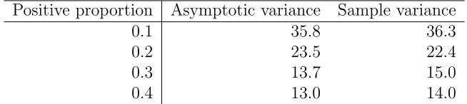
We can see that the risk score functions obtained from either maximizing AUCPR or AUCROC are quite close to the optimal one, leading to the similarity in the false discovery rate by each approach. However, the smaller MSE as well as a smaller standard deviation for Precision-Recall one indicates that maximizing AUCPR is more efficient. Furthermore, we vary the proportion of positive examples to obtain the sample variance as well as the asymptotic variance of the Precision-Recall estimate through referring to Theorem 1. Table 2.3 indicates a close result between the two.

Table 2.3: Comparison between asymptotic and sample variance of PR estimate under simulation Model I.

Positive proportion Asymptotic variance Sample variance

0.1 35.8 36.3

0.2 23.5 22.4

0.3 13.7 15.0

0.4 13.0 14.0

2.4.2

Simulation Model II

The second configuration with the sample sizen= 400 and proportion of positive examples

π = 20% is to generate the predictors according to X|Y = 1 ∼ BN(0,0,2,0.5,0) and

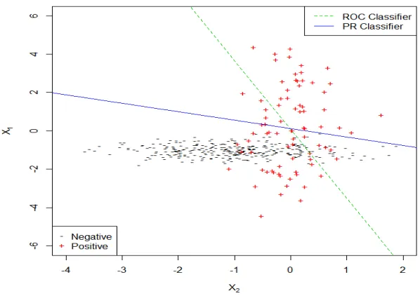
X|Y = 0∼BN(−1,−1,0.3,1,0). By the Neyman-Pearson lemma, because of non-equal variances, the UMP test suggests to use the quadratic score function 391X₁2−108X₂2+ 800X1+ 72X2. However, in practice, linear classifiers are often used. Considering using

X1+ 3.59X2. Note that these solutions differ significantly. The angle between the two

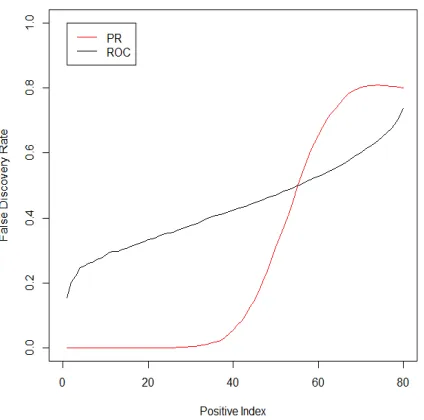
lines is 43◦. Figure 2.2 shows the scatter plot of the example dataset with PR and ROC linear classifiers, which are just the direction instead of the particular lines. Here we display the classifiers with thresholds that pick out half of the true positives by each method. Estimation results are summarized in Table 2.4, where the standard deviation for each coefficient estimate is in the parenthesis. To compare the two classifiers, we consider the false discovery rate for each classifier as a function of the number of true positive discoveries. Figure 2.3 shows the false discovery rate by both PR and ROC methods.

Figure 2.2: Scatter plot of the example dataset with PR and ROC linear classifiers under simulation Model II.

If the goal is to control the false discovery rate at a reasonable level, which is often the case, then the Precision-Recall approach stands out with a much smaller false discovery rate compared to the ROC, crossing when the false discovery rate reaches about 50% and approximately 75% of the true positives are found.

Table 2.4: Estimates of the risk score function by PR and ROC methods under simulation Model II.

Curve β0 β1

PR 1 (0) 0.4418 (0.1075) ROC 1 (0) 3.5936 (1.5326)

methods, the Precision-Recall approach suggests to use X1 + 0.43X2 while the ROC

method proposes X1+ 3.27X2, similar to the results from the sample. Once we project

down to the linear combination, since the optimal classifier is quadratic, we can consider constructing a quadratic classifier in the form of (X1 + 0.43X2)2+a(X1+ 0.43X2) from

the linear classifier suggested by the PR curve, and compute the maximum area under the PR curve and ROC curve respectively by optimizing overa. Similarly, we can also construct a quadratic classifier (X1+ 3.27X2)2+b(X1+ 3.27X2) based on the ROC result,

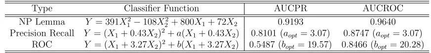
compute the maximum area under each curve by optimizing over b. After the tuning procedure, the optimal a and b are found to maximize the area under the curve with results summarized in Table 2.5.

Table 2.5: Comparison in the area under the PR and ROC curve among different classifiers.

Type Classifier Function AUCPR AUCROC

NP Lemma Y = 391X2

1−108X 2

2+ 800X1+ 72X2 0.9193 0.9640

Precision Recall Y = (X1+ 0.43X2)2+a(X1+ 0.43X2) 0.8101 (aopt= 3.07) 0.8747 (aopt= 3.07)

ROC Y = (X1+ 3.27X2)2+b(X1+ 3.27X2) 0.5487 (bopt= 19.57) 0.8466 (bopt= 20.28)

It can be seen that the binormal Precision-Recall method outperforms binormal ROC method in terms of larger area under the curve, including both AUCPR and AUCROC. Although the optimal classifier is quadratic, if we want to simplify the classification problem by using linear classifier, it is suggested to use the risk score function generated by maximizing AUCPR, instead of AUCROC. By Precision-Recall method, not only we can better control the false discovery rate, but we can gain a larger area under the curve through constructing a quadratic classifier from a linear one as well.

2.4.3

Simulation Model III

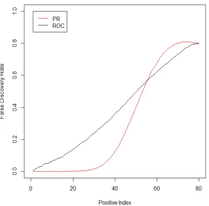
X2|Y = 1 ∼0.95N(−0.8,1.2) + 0.05N(1.5,0.2). Figure 2.4 displays the false discovery

rate by both PR and ROC methods, indicating a substantial improvement using the Precision-Recall approach over the ROC method in terms of the classification performance while controlling the false discovery rate at a low level.

Figure 2.4: False discovery rate by PR and ROC methods under simulation Model III.

2.5

Real data analysis

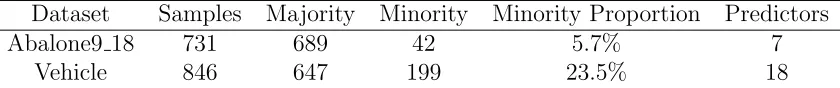
Siebert (1987), involving classification of a given silhouette as one of four types of vehicles based on a set of 18 continuous features. In order to make the data imbalanced, we follow Fan et al. (2014) to choose class label “van” as the minority class with ratio 23.5%. The data is summarized in Table 3.1.

Table 2.6: Characteristics of datasets.

Dataset Samples Majority Minority Minority Proportion Predictors

Abalone9 18 731 689 42 5.7% 7

Vehicle 846 647 199 23.5% 18

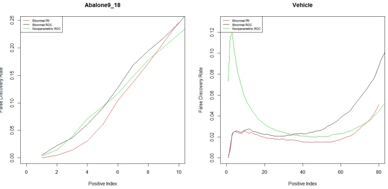
For each data set, we randomly split both the majority group and minority group into two parts evenly, forming a training dataset consisting of half of majority samples and half of minority samples, as well as a testing dataset with the other halves. Besides the binormal Precision-Recall method and binormal ROC method discussed above, we also implement the non-parametric approach to maximize AUCROC, which uses a sigmoid approximation without the binormal assumption (Ma and Huang, 2005). The three methods are conducted on the training data set to estimate their corresponding linear classifiers with performance measured on the testing data set based on 200 repetitions, where the relationship between average false discovery rate and true positive (minority) examples are shown in Figure 2.5.

For the Abalone9 18 data, the binormal Precision-Recall approach performs best among the three in terms of controlling false discovery rate at a lower level, up to around 20% in classification of correctly identifying 50% of the minority class. For the Vehicle data, each of the three methods does a good job because of the low false discovery rate, but comparatively the binormal Precision-Recall approach outperforms the binormal ROC over the full range, while outperforming the non-parametric approach when successfully finding 80% of the minority examples in the testing data set.

2.6

Discussions

Figure 2.5: Relationship between average false discovery rate and true positive examples.

distribution of the estimate has been derived and compared with that in the binormal ROC approach. Simulation as well as real data results indicate that the binormal Precision-Recall approach has an improvement over the binormal ROC method and the TGDR algorithm in terms of controlling the false discovery rate at a lower level and a smaller asymptotic variance for the estimates in the classifier.

CHAPTER

3

Feature Selection for Imbalanced Data

3.1

Introduction

Feature or variable selection, whose purpose is to eliminate irrelevant variables to enhance the generalization performance of a given learning algorithm, is an important topic in ma-chine learning, especially in high dimensional applications. In regression and classification problems with a large number of predictors, if only some of the variables contribute to the response, overfitting appears to be a critical concern for statistical analysis. Consequently, finding the optimal subset of variables among the pool is necessary and momentous.

etc. Maldonado et al. (2014) designed a feature selection method for high-dimensional class-imbalanced data sets using SVM. Since the receiver operating characteristic (ROC) curve (Hanley and McNeil, 1982) plays an important role in measuring the performance of a binary classifier system as its decision threshold is varied, Ma and Huang (2005) applied a sigmoid approximation to the empirical area under the ROC curve (AUCROC) as the objective function for classification and implemented the threshold gradient descent regularization (TGDR) algorithm (Friedman and Popescu, 2003) for estimation and variable selection in the linear risk score function. However, ROC curves tend to present an overly optimistic view of an algorithm’s performance in terms of classification of highly imbalanced data (Davis and Goadrich, 2006). Precision-Recall (PR) curves (Raghavan et al., 1989), an alternative to ROC curves for tasks with imbalanced data, have become a basis for assessing classification methods. Consequently, Liu and Bondell (2016) proposed a classification algorithm with imbalanced data based on estimating the risk score function via maximization of the area under the Precision-Recall curve (AUCPR) in a binormal framework (Brodersen et al., 2010b).

In this chapter, we propose a regularized binormal Precision-Recall algorithm for variable selection in the classification context. It consists of two stages. The first stage is to compute the area under the Precision-Recall curve (AUCPR) in a binormal framework. With the binormal AUCPR criterion, we apply the threshold gradient descent regular-ization (TGDR) method for variable selection, which is the second stage. The proposed variable selection approach works well, especially when facing class-imbalanced data sets. We demonstrate via both simulations and real data analysis, that our method outperforms that based on the area under the ROC curve.

The chapter is organized as follows. Section is devoted to illustrating the proposed regularized binormal Precision-Recall algorithm. Two simulation settings are presented in section and real data analysis is discussed in section . Section gives discussions.

3.2

Regularized Binormal Precision-Recall Algorithm

For j = 0,1, we denote µ_j = E(X|Y = j) and Σj = Var(X|Y = j). We assume that

µ₀, µ₁, Σ0 and Σ1 exist, and at least one of {Σ0,Σ1} is non-singular. (Liu and Bondell,

Equation (2.4), is given by

β_ROC ∝(Σ1 + Σ0)−1(µ1−µ0). (3.1)

However, in order to maximize AUCPR, defined in Equation (2.6), we solve it numeri-cally via algorithms such as gradient descent because there is no closed-form solution. In practice, (µ₀,µ₁,Σ0,Σ1) is replaced by its sample counterpart ( ¯X0,X¯1, S0, S1).

3.2.1

Anchor Variable

Since both ROC and PR estimators consider the full range of thresholds, c, the vector β

is only identifiable up to a scalar multiple. For identifiability, prior to analysis, we need to define the anchor variable, the one whose estimated coefficient will be set as a constant. This is the same as the anchor biomarker in the biology field. Ma et al. (2006) used an adjusted t-statistic, similar to a simple shrinkage method (Cui et al., 2005), to define the anchor biomarker. In this thesis work, we fix the anchor variable such that |βanchor|= 1. In the PR approach, we compute the AUCPR according to (2.6) by using each variable separately, and the anchor variable is defined as the one with maximum AUCPR. Similarly, in the ROC method, the anchor variable is defined as the one with maximum AUCROC in (2.4).

3.2.2

Threshold Gradient Descent Regularization (TGDR)

β(v) denote the parameter path indexed by v ∈ [0,∞), ∆v denote the infinitesimal positive increment as in ordinary gradient descent methods. For any threshold τ ∈[0,1], the TGDR algorithm is described as follows.

In the solution path, the anchor variable will always be the first one to be selected because we set its gradient at 0 in every iteration, and its magnitude is fixed at 1. The number of iterationsK and threshold τ jointly determine the property of other estimated

β. When τ ≈ 0, ˆβ is dense for all values of K. On the contrary, when τ ≈ 1, then ˆβ

Algorithm 1 TGDR

1: procedure TGDR

2: Initialize β(0) =0 and v = 0, except that |βanchor|= 1.

3: repeat

4: Compute the negative gradientg(v) =−∂R(β)/∂β evaluated at β(v). Denote the i-th component of g(v) as gi(v), and set the component for anchor variable at 0. If maxi{|gi(v)|}= 0, stop the iteration.

5: Compute the vector f(v) with the i-th component fi(v) = I{|gi(v)| ≥ τ · maxi|gi(v)|}, an indicator function.

6: Update β(v+ ∆v) =β(v)−∆v×g(v)×f(v) and replace v by v+ ∆v, where the product of f and g is componentwise.

7: until K times, a large number to guarantee a full parameter path.

8: Output nonzero β’s in β.

9: end procedure

will become dense eventually. At the extreme case, i.e. τ = 1, the TGDR algorithm usually increases in the direction of a single covariate in each iteration, which mimics the incremental forward stagewise strategy (Hastie et al., 2005). When τ is in the middle range, the characteristics of β are between those for τ = 0 and τ = 1. Friedman and Popescu (2003) used cross validation techniques to tune the parametersK and τ.

3.2.3

Regularized Binormal Precision-Recall Algorithm

The regularized binormal Precision-Recall algorithm is a combination of the area under the binormal Precision-Recall curve, defined in (2.6), and the threshold gradient descent regularization method described above. In other words, the regularized binormal Precision-Recall algorithm is the TGDR approach with binormal AUCPR as the objective function, i.e.

RP R(β) =

Z

0

πt

πt+ (1−π)Φ

βT(µ₀−µ₁)

q

βTΣ0β

+ q

βTΣ1βΦ−1(t)

q

βTΣ0β

And the negative gradient at β is given by

−∂RP R(β)

∂β =

Z 1

0

π(1−π)tφ(T1)(T2+T3)

(πt+(1−π)Φ(T1))2 dt, (3.3)

where T1 = β

T

(µ₀−µ₁)

q

βTΣ0β

+ q

βTΣ1βΦ−1(t)

q

βTΣ0β

,

T2 =

(µ₀−µ₁)βTΣ₀β−βT(µ₀−µ₁)Σ₀β

βT

Σ0β

3/2 ,

T3 = Φ−1(t)Σ1ββ

T

Σ0β−β

T

Σ1βΣ0β

βTΣ0β

3/2

βTΣ1β

1/2 .

In conclusion, we apply the TGDR algorithm to maximize the AUCPR in (3.2) with the negative gradient function in (3.3), record the parameter solution path and select important variables.

Similarly, based on the binormal AUCROC in (2.4), the regularized binormal ROC algorithm applies the TGDR algorithm to maximize (3.4) with the negative gradient function in (3.5).

RROC(β) = Φ





βT(µ₁−µ₀)

q

βT(Σ1+ Σ0)β 

. (3.4)

−∂RROC(β)

∂β =φ





βT(µ₁−µ₀)

q

βT(Σ1+ Σ0)β 



βT(µ₁−µ₀)(Σ1+ Σ0)β−(µ1−µ0)β

T

(Σ1+ Σ0)β βT(Σ1+ Σ0)β

3/2 .

(3.5)

3.3

Simulation

algorithm, we fix τ = 1 to guarantee the sparse solution and K = 5000, which is large enough to produce a full parameter path for our settings. In the second stage, we follow the solution path and sequentially use a certain number of selected variables to implement the classification on a simulated large testing data set, and compare the performance between the two methods. The false discovery rate (FDR) in Equation (2.7) and the false positive rate (FPR) in Equation (2.1) are used as measures of the variable selection effectiveness of each method. The simulation settings consider the normal and non-normal situations respectively.

3.3.1

Simulation Model I

In the first configuration, we use variable size p= 10 and proportion of positive examples

π = 20%. Both the training data set with the sample size n= 400 and the testing data set with the sample size n= 10000 are to generate the first two predictors according to binormal distributions (BN), i.e.

(X1, X2)T|Y = 0∼BN

0 0

!

, 0.5 0

0 0.1

!!

,

(X1, X2)T|Y = 1∼BN

0.5 0.5

!

, 0.4 0.9

0.9 2.5

!!

,

and other covariates X= (X3,· · · , X10)T in both negative group (givenY = 0) and

posi-tive group (given Y = 1) are generated from a common multivariate normal distribution with mean vector 2 and compound symmetric covariance matrix Σ, where ρ= Σij = 0.4, when i6=j.

Based on the Neyman-Pearson theory (Neyman and Pearson, 1992), the optimal risk score function via the most powerful test in this setting only consists of the first two variables, X1 and X2, because of the common probability density function form

for the other covariates. The training data set is generated repeatedly for 100 times, where we apply the regularized binormal PR algorithm and the regularized binormal ROC algorithm as well as record the solution path on each simulated training data. The PR-based algorithm always regards X2 as the anchor variable and the second selected

always choosesX1 as the anchor variable, while the second selected variable in the solution

path varies.

Following the solution path generated by each algorithm, we consider using linear functions to do the classification on the testing data set with the sample size n= 10000. Start from using the anchor variable only, we sequentially add one variable in the existing classifier. To compare the two classifiers, we consider the false discovery rate for each classifier as a function of the proportion of true positive discoveries, as well as the false positive rate for each classifier as a function of the proportion of true positive discoveries. Figure 3.1 and 3.2 respectively show the false discovery rate and false positive rate by using the two algorithms.

In practice, when facing imbalanced data, the goal is often to control the false discovery rate or false positive rate at a reasonable level. Figure 3.1 tells us that the Precision-Recall algorithm stands out with a much smaller false discovery rate compared to the ROC, crossing when the false discovery rate reaches about 70% and approximately 60% of the true positives are found. In addition, Figure 3.2 shows that the PR has a smaller false positive rate before it reaches 35%. The trend is already obvious when only using one variable in the classifier. The performance is slightly improved when using two variables (X2 and X1) in the PR-based classifier, while more variables do not help any more.

In conclusion, the regularized binormal PR algorithm selects X2 andX1 as the

impor-tant variables, which is consistent to the Neyman-Pearson theory, while the regularized binormal ROC algorithm fails in terms of variable selection in this setting. It is also suggested to follow the solution path generated by the regularized binormal PR algorithm to create classifiers in order to better control the false discovery rate and false positive rate in dealing with imbalanced data sets.

3.3.2

Simulation Model II

sample size n= 10000 according to

(X1, X2)T|Y = 0∼BN

0 0

!

, 1.44 0

0 0.1225

!!

,

X1|Y = 1∼0.95N(1,1) + 0.05N(−1,0.04),

X2|Y = 1∼0.95N(−0.8,1.44) + 0.05N(1.5,0.04).

and other covariates X= (X3,· · · , X10)T in both negative group (givenY = 0) and

posi-tive group (given Y = 1) are generated from a common multivariate normal distribution with mean vector 2 and compound symmetric covariance matrix Σ, where ρ= Σij = 0.4, when i6=j.

Following the same two-stage procedure as in simulation model I, the regularized binormal PR algorithm picks X2 as the anchor variable and X1 as the second important

variable in each repetition, and it also appears to be (X2, X1) or (X1, X2) in the solution

path of the regularized binormal ROC algorithm. Although both algorithms catch the right important variables (X2 and X1) during the early stage of the solution path, consistent

to the Neyman-Pearson result, the classification performances on the testing data set by classifiers of the two algorithms differ a lot in terms of false discovery rate and false positive rate, shown in Figure 3.3 and 3.4.

Figure 3.3 and 3.4 indicate a substantial improvement using the regularized binormal PR algorithm over the ROC-based method in terms of the classification performance while controlling the false discovery rate as well as the false positive rate at a low level. The Precision-Recall algorithm produces a smaller false discovery rate than the ROC algorithm when it reaches around 70%, and a smaller false positive rate when it reaches nearly 40%. The difference between performances of two algorithms has been significant since using only one variable in the classifier. Furthermore, classifiers with two variables are better than one variable model for both methods, but this difference remains constant since three variables.

To sum up, in this non-normal setting, although both the regularized binormal PR and ROC algorithm select the same important variables, X2 andX1, the PR algorithm

3.4

Real Data Analysis

To illustrate the variable selection performance of the regularized binormal Precision-Recall algorithm, we analyze the Abalone real data set (Nash, 1994), aiming to predict the age of abalone from 7 continuous physical inputs. The data is from the UC Irvine machine learning repository (Bache and Lichman, 2013), and according to Fan et al. (2014), we transformed it to a highly imbalanced binary classification data set called Abalone9 18 by focusing only on those observations with class label “9” (young group) and “18” (old group), regarding class 18 as the minority class with proportion 5.7%. The data is summarized in Table 3.1.

Table 3.1: Characteristics of Abalone9 18 data set.

Data Samples Majority Minority Minority Proportion Predictors

Abalone9 18 731 689 42 5.7% 7

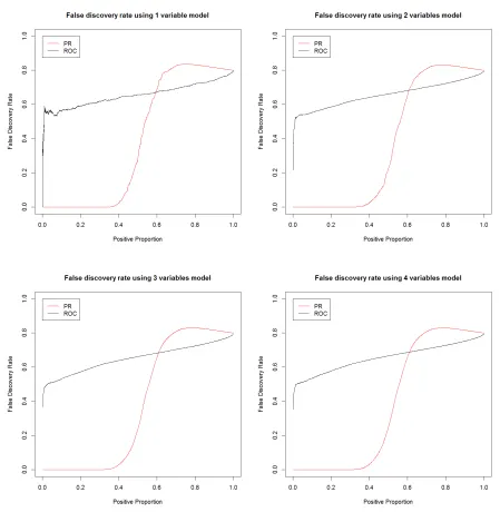
We randomly split both the majority group and minority group in the data set into two parts evenly, forming a training dataset (365 samples) consisting of half of majority samples (344 negatives) and half of minority samples (21 positives), as well as a testing dataset (366 samples) with the other halves (345 negatives and 21 positives). Similar to the two-stage procedure in the simulation study, we apply the proposed regularized binormal PR algorithm and the regularized binormal ROC algorithm on the training data set to obtain the solution path with threshold τ = 1 and iterations K = 10,000. Afterwards we sequentially use the first 4 variables in the solution path to implement the classification on the testing data set, and compare the performance between the two methods. Figure 3.5 and 3.6 respectively show the false discovery rate (FDR) and false positive rate (FPR) as a function of positive proportion by using the two algorithms based on 200 repetitions.

classification. No matter how many variables are used for classification, the regularized binormal PR algorithm significantly outperforms the ROC algorithm almost over the full range. Figure 3.7 and 3.8 show 95% confidence intervals for the mean difference of FDR and FPR between the two methods separately. The mean difference, drawn in red solid lines, is negative almost over the full range. In the meantime, the 95% confidence intervals, drawn in black dashed lines, does not contain 0, further indicating the significance of better performances using the proposed regularized binormal PR algorithm.

3.5

Discussions

It is of practical importance to develop an efficient feature selection approach for class-imbalanced data. In this chapter, we propose a regularized binormal Precision-Recall algorithm for variable selection in the classification context, which applies the threshold gradient descent regularization (TGDR) method to maximize the area under the Precision-Recall curve (AUCPR) in a binormal framework. Simulation as well as real data results indicate that the regularized binormal Precision-Recall algorithm has an improvement over the regularized binormal ROC method when facing imbalanced data in terms of controlling the false discovery rate and false positive rate at a lower level.

CHAPTER

4

Variable Screening in Ultrahigh Dimensions

4.1

Introduction

We consider the problem of ultrahigh dimensional regression, i.e. the dimension of pre-dictors used for predicting a response of interest, p, is much larger than sample size, n. It is often assumed that only a relatively small subset of the predictors contribute to the response. As a result, an efficient method of variable selection, which can be able to identify the most important predictors, plays an key role in the ultra-high dimensional regression.

One group of variable selection methods are based on penalized methods which can select variables and estimates parameters simultaneously through solving an ultrahigh dimensional regression with some pre-specified penalties leading to sparsity. These methods include bridge regression (Frank and Friedman, 1993), LASSO (Tibshirani, 1996), SCAD (Fan and Li, 2001), Dantzig selection (Candes and Tao, 2007), and other folded concave regularization methods (Fan and Lv, 2011; Zhang and Zhang, 2012). When the dimension is very high, however, these methods may have heavy implementation cost and face challenges in computational feasibility.

and Lv, 2008), marginal bridge regression based method (Huang et al., 2008) and some others. Specifically, SIS method in (Fan and Lv, 2008) selects important variables in an ultrahigh dimensional linear models based on the marginal correlations of each predictor with the response. They showed that the correlation ranking of the predictors possesses a sure independence screening property, that is, the important variables can be selected with probability close to one. Later, the marginal screening method was extended to generalized linear models (Fan and Song, 2010). Various screening methods have been developed, to name a few, tilting methods (Hall et al., 2009), generalized correlation screening (Hall and Miller, 2009), nonparametric screening (Fan et al., 2011), robust rank correlation based screening (Li et al., 2012), and quantile-adaptive model-free feature screening (He et al., 2013).

These marginal screening methods face a number of challenges. For example, if the marginal working model is too far away from the true model, it is hard to ensure the sufficient conditions for sure screening to hold. Consequently marginally unimportant but jointly important variables may not be preserved in marginal screening. Meanwhile, the marginal screening methods may include noise variables that are weakly correlated with the important predictors. It can potentially increase false positive rate.

To address these issues, in this chapter, we propose a principal component-adjusted screening (PCAS) method for generalized linear models. The key idea is to use principal components as surrogate covariates to account for omitted covariates in marginal screening. Specifically, we fit pmarginal regressions by maximizing the marginal likelihood including not only the screened predictor but also some selected principal components. Then we consider an independence learning by ranking the maximum marginal likelihood estimators or maximum marginal likelihood.

implementation only requires eigenvalue-decomposition of an n by n matrix regardless of the dimensionalityp.

The setup of generalized linear models is introduced in section 4.2. Section 4.3 discussed the computation of principal components. In section 4.4, we introduced the PCAS procedure with maximum marginal likelihood estimators (MMLE) and marginal likelihood ratio (MLR). Simulation results are presented in section 4.5 and two real data analysis results are illustrated in section 4.6. Section 4.7 gives concluding remarks.

4.2

Generalized linear models

Consider the generalized linear model where the probability density function of a response variable Y takes the form fY(y;θ) = exp{yθ−b(θ) +c(y)}, with known functions b(·),

c(·), and the natural parameter θ. Suppose that the observed data{(Xi, Yi), i= 1,· · · , n} are identically independent distributed copies of (X, Y), whereXi = (1, Xi1,· · · , Xip)T and Xi1,· · ·, Xip are p-dimensional covariates for subject i. β = (β0, β1,· · ·, βp)T is a (p+ 1)-vector of parameter. We are interested in identifying the sparsity structure of β

from the equation

E(Y|X=x) =b0(θ(x)) = g−1( p

X

j=0

βjxj), (4.1)

wherex={x0, x1,· · · , xp}T is a (p+ 1)-vector withx0 = 1 when considering the intercept,

b0(θ) is the first order derivative of b(θ) with respect toθ and g is the link function. For demonstration purpose, in the thesis work we only take canonical link function, that is

g = (b0)−1, into consideration. In this case, θ(x) = p

P

j=0

βjxj. The ordinary linear model

Y =XTβ+ε, where ε is the random error, is a special case of model (4.1) by using the identity link, i.e. g(µ) = µ. Considering binary response data, the logistic regression is another special case of model (4.1) by using the logit link g(µ) = log(µ/(1−µ)).

4.3

Principal component analysis

dataset to another coordinate system by determining the eigenvectors and eigenvalues of the matrix, principal component analysis involves calculations of a covariance matrix of a dataset to minimize the redundancy as well as maximize the variance (Shlens, 2014). A common method to find the eigenvectors and eigenvalues is singular value decomposition (SVD), which decomposes a matrix into a set of rotation and scale matrices. SupposeXis a matrix withnrows andpcolumns and columns are normalized to be norm one. A singular value decomposition of X is given by Xn×p = Un×n(diag(λ1, . . . , λn),0n×(p−n))VTp×p, where U and V are orthonormal matrices with dimensions n and p respectively and diag(λ1, . . . , λn) is a diagonal matrix with diagonal elements λ1, . . . , λn. Additionally,

λ1 ≥λ2 ≥. . .≥λn ≥0. Since

XTX=Vdiag(λ2₁, . . . , λ2_n,0, . . . ,0)VT,

it is clear that the columns of V are the principal directions of X. Thus, the prin-cipal components, that is, the projection of X’s rows on these directions, should be

XV =Un×ndiag(λ1, . . . , λn). In other words, each column of Urepresents each principal

component up to some scale.

To calculate U, we note XXT =Udiag(λ2

1, . . . , λ2n)U

T_{. Therefore, if we perform an} eigenvalue decomposition onXXT, which is a matrix with much smaller dimensions when

p is much larger than n, then U0s columns consist of all eigenvectors.

4.4

PCAS procedure

4.4.1

PCAS with maximum marginal likelihood estimators

j , for j = 1, . . . , p, is defined as the minimizer of the negative marginal log-likelihood

( ˆβ_j,M₀,βˆ_jM,γˆM_j,1, . . . ,ˆγ_j,KM

n)

T _{= argmin} β0,βj,γj,1,···,γj,Kn

Pnl(β0 +βjXj + Kn

X

k=1

γ_j,kMUk, Y),

forj = 1, . . . , p,

where l(Y;θ) = −(θY −b(θ) +c(Y)),{Uk} is the kth eigenvector consisting of {Uik}ni=1,

and _Pnf(X, Y) =n−1

Pn

i=1f(Xi, Yi) is the empirical measure. ˆβjM measures the strength of the conditional contribution of Xj given the first Kn principal components. These principal components represent the information of predictors except forXj in the marginal model. The process can be rapidly computed.

Specifically, in ordinary linear models with normality assumption of random errors, the maximum likelihood estimator is identical to the ordinary least squares estimator written as

( ˆβ_j,M₀,βˆ_jM,γˆ_j,M₁, . . . ,ˆγ_j,KM

n)

T _{= argmin} β0,βj,γj,1,···,γj,Kn

Pn(Y −β0−βjXj− Kn

X

k=1

γ_j,kMUk)2,

forj = 1, . . . , p.

We select a set of variables

c

Mγn ={1≤j ≤p:|βˆ

M

j | ≥γn}, (4.2)

Since the rationale to use the principal components as surrogate covariates is to account for the effect of the omitted covariates in the marginal model, we should compute the principal components based on the p−1 omitted covariates for each marginal regression. For simplicity of computation, we compute the principal components based on all p

covariates and use these principal components as surrogate covariates. Based on our observations, the numerical performance of two methods are very close while the latter one has significantly smaller computational costs.

4.4.2

PCAS with marginal likelihood ratio

As an alternative method, we can also rank variables based on the likelihood reduction of the variable Xj given the first Kn principal components, which we call PCAS with maximum likelihood ratio (PCAS-MLR):

Lj,n =Pn{l( ˆβjMXj + Kn

X

k=1

ˆ

γ_j,kMUk, Y)} −Pn{l( ˆβ0M, Y)}, forj = 1, . . . , p,

where ˆβM

0 = argmin

β0

Pnl(β0, Y). Denote Ln= (L1,n, L2,n,· · · , Lp,n)T. Specifically, in ordi-nary linear models,

Lj,n =Pn{(Y −βˆjMXj −

PKn

k=1ˆγj,kMUk)2} −Pn{(Y −βˆ0M)2}, forj = 1, . . . , p,

where ˆβM

0 = argmin

β0

Pn(Y −β0)2.

The smaller the Lj,n is, the more the variableXj contributes. We sort the vectorLn in an ascending order and choose variables according to

b

Nνn ={1≤j ≤p:Lj,n ≤νn}, (4.3)

4.4.3

Determining the number of selected variables

It remains open on how to choose the number of selected variables d in variable screening literature. In applications, it is common for practitioners to select a prefixed number of top-ranked variables, as the prefixed number may reflect prior knowledge of the number of susceptible predictors or budget limitations. Another commonly used procedure is to set the size of the selected set to a number less than the sample size, for example

d = [2n/log(n)] (Fan and Lv, 2008), so that the follow-up analysis can be performed in a p < nscenario. Data-driven procedures for determining the size of the important set are appealing but relatively limited. They include information criteria, such as AIC and BIC, and the false discovery rate (FDR) based methods (Barut et al., 2012; Zhao and Li, 2012). These methods, however, have large computational cost, especially in the ultra-high dimensional framework. Following (Fan and Lv, 2008), we used d= [2n/log(n)] in this thesis.

4.4.4

Determining the number of principal components

The choice of numbers of principal components Kn is critical for PCAS. We propose to use the following two data adaptive methods. The first method is the scree plot, a classical method in factor analysis to determine the number of principal components. As a related numerical method, we can also use the maximum eigenvalue ratio criterion (Luo et al., 2009), defined asλj/λj+1 with 1≤j ≤n−1 and λ1 ≥λ2 ≥. . .≥λn>0. We choose the number of principal components that can maximize the eigenvalue ratio, that is,

ˆ

k= argmax_1≤j≤kmax(λj/λj+1), (4.4)

where kmax ≤ n is a prespecified maximum factor dimension. When the predictors’

correlation structure follows a factor model, it was shown in Wang (2012) that ˆk is consistent to the dimension of the linear subspace spanned by the column vectors of factors’ matrix.

4.5

Simulations