Article
Interpolation of Instantaneous Air Temperature using
Geographical and MODIS derived variables with
Machine Learning Techniques
Marcos Ruiz-Álvarez1,‡ ID, Francisco Alonso-Sarria2,‡,∗, Francisco Gomariz-Castillo3,‡
1 Instituto Universitario de Agua y Medio Ambiente. Universidad de Murcia. Campus de Espinardo, 30001,
Murcia, Spain; [email protected]
2 Instituto Universitario de Agua y Medio Ambiente. Universidad de Murcia. Campus de Espinardo, 30001,
Murcia, Spain; [email protected]
3 Instituto Euromediterráneo del Agua. Campus de Espinardo, 30001, Murcia, Spain; [email protected]
* Correspondence: [email protected]; Tel.: +34-868-888-695 ‡ These authors contributed equally to this work.
Abstract:Several methods have been tried to estimate air temperature using satellite imagery. In
this paper, the results of two machine learning algorithms, Support Vector Machine and Random
Forest, are compared with Multivariate Linear Regression, TVX and Ordinary kriging. Several
geographic, remote sensing and time variables are used as predictors. The validation is carried out
using four different statistics on a daily basis allowing the use of ANOVA to compare the results.
The main conclusion is that Random Forest with residual kriging produces the best results (R2=0.612
±0.019, NSE=0.578±0.025, RMSE=1.068±0.027, PBIAS=-0.172±0.046), whereas TVX produces
the least accurate results. The environmental conditions in the study area are not really suited to
TVX, moreover this method only takes into account satellite data. On the other hand, regression
methods (Support Vector Machine, Random Forest and Multivariate Linear Regression) use several
parameters that are easily calculated from a Digital Elevation Model, adding very little difficulty
to the use of satellite data alone. The most important variables in the Random Forest Model were
satellite temperature, potential irradiation and cdayt, a cosine transformation of the julian day.
Keywords:Air temperature, MODIS, machine learning, interpolation
1. Introduction
Air temperature (Ta) is a very relevant climatic variable that controls several environmental
processes, particularly evapotranspiration [1]; it is also a key feature in global change studies, and
reflects the surface energy balance [2]. So, accurate estimations ofTaand its spatio-temporal variability
are important in several Earth and environmental sciences and in land surface process modelling
[1,3]. Air temperature is usually measured in weather stations at a standard height of 1.5-2 m with
diverse temporal resolutions. However, because weather stations provide limited information about
spatial patterns at regional or global scales [3], several methods have been used to estimate the spatial
distribution ofTa[4,5]:
• Vertical lapse methods [4] use height as the main variable to explain temperature spatial
distributions. The vertical lapse rate is evaluated from the sampling data and then applied
to the whole study area. A more sophisticated approach uses daily atmopspheric profiles
provided by the MODIS product MOD07_L2 to locally estimate the adiabatic lapse rate [6]. The
main drawback of this approach is that spatial resolution is 5 km.
• Simple linear regression using land surface temperature (LST), retrieved by remote sensing, as
a predictor forTa[7]. MODIS, for example, provides global coverage of several environmental
variables with large temporal resolution and moderate spatial resolution [6].
• Multivariate regression models using LST and other variables such as NDVI, solar zenith
angle, solar radiation, altitude, julian day, distance to the coast, normalized difference water
index (MNDWI) or albedo as predictors [8–15]. The algorithms used range from multivariate
linear regression [5,10,11,16] to more sophisticated machine learning algorithms, such as neural
networks [9] or random forest (RF) [14].
• Geostatistical techniques (kriging) [17,18] estimate Ta as a weighting average of the sampling
points with the weighting coefficients obtained after a statistical analysis of the spatial variability
of the variable (semivariogram functions).The main drawbacks of such interpolation methods
are that they do not use covariates and that they may have uncertainties due to the clustered
distribution of weather stations [19].
• The Temperature-Vegetation Index (TVX), proposed by [20] and [21], is based on the correlation
between NDVI and LST, assuming thatTais approximately equal to LST in fully vegetated areas.
Significant uncertainties appear in sparse vegetation areas [22].
• Methods based on the surface energy balance such as ADEBAT [4,13]. The objective is to approach
Taestimation from a more physical point of view. It has two main drawbacks: several variables
that can only be measured in weather stations are needed and, as the Bowen ratio is one of them,
it is necessary to know LE to use ADEBAT. Frequently,Tais estimated in order to estimate LE
from it, as i -l spa -psm 3 n our case, so the use of a surface energy balance is not suitable in this
case for practical reasons.
Remote sensing methods are constrained by the time of the day when images are taken. During
the night, LST is a very accurate proxy forTaas solar radiation has no effect, simplifying the ground
surface energy balance. During the day, it is necessary to take into account several variables, such as
[23]showed that correlation between LST at night and minimumTais higher (R2=0.93) than between
their daytime equivalents (R2=0.79).
The objective of this work was to use two well known machine learning algorithms, Support
Vector Machines (SVM) and RF, to estimateTaat the AQUA passage time (between 12:00 and 14:20)
using all the variables included as predictors in previous works. The results are compared to those
obtained with more traditional approaches: Multivariate linear regression, Ordinary Kriging (OK)
and TVX. Finally, regression-kriging will be tested using OK to interpolate the residuals of the three
regression models, provided that such residuals show spatial autocorrelation.
2. Methodology
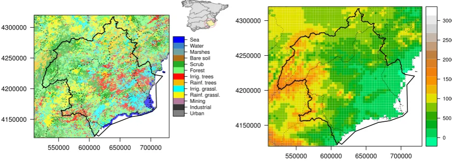
2.1. Study area
This research was carried-out in the area controlled by the River Segura Water Authority (DHS in
its Spanish abbreviation) (figure1), which includes the Segura river basin (19,000 km2) and several
minor coastal basins. It is a semiarid area with scarce and irregular precipitation, high temperatures,
and a large number of hours of sun that cause high potential evapotranspiration. Despite the scarcity
of water, agriculture is an important economic sector using both groundwater (available because the
predominance of carbonate rocks) and water transferred from other basins. Population density and
intensive irrigated agriculture represent a significant water demand.
The study area is also characterised by substantial height differences over short distances, which
together with the semiarid climate and the use (limited in space) of groundwater and transferred water,
create a strong environmental variability that represents unfavourable conditions for the use of TVX.
4150000 4200000 4250000 4300000
550000 600000 650000 700000
Urban Industrial Mining Rainf. grassl. Irrig. grassl. Rainf. trees Irrig. trees Forest Scrub Bare soil Marshes Water Sea
4150000 4200000 4250000 4300000
550000 600000 650000 700000
0 500 1000 1500 2000 2500 3000
2.2. Data set
Different variables were used as predictors: 1. geographical variables: longitude, latitude, altitude,
TWI index [24] (used to describe the potential accumulation of cold air), monthly potential irradiation
(Whm−2month−1) obtained from heights using the method proposed by [25] and distance from the
coast; 2. time variables: day duration, cdayt (a cosine transformation of julian day following [26],
equation3) and the satellite passage time; and 3. variables provided by the MODIS sensor: EVI, Albedo
and the terrestrial surface temperature (LST) at the passage time of AQUA satellite.
The equation to calculate cdayt is:
cdayt=cos[tD−φ]· 2π
365
(1)
wheretDis the julian day andφis a time delay from the coldest day.
2.2.1. Weather data
Air temperature data every 30 minutes is recorded by 53 weather stations belonging to the SIAM
and SIAR networks (Sistema de Información Agrometeorológico de la Región de Murcia, Agro-meteorological
information System in Murcia Region) and Sistema de Información Agroclimática para el Regadio,
Agro-meteorological Information System for Irrigation). In this work, only data for 2012 were analysed
to test which model produces the most accurate results, .
We assumed that the mean air temperature data (obtained from the average of 3 measurements
taken every 10 minutes) provided by the SIAR and SIAM networks are equal to the air temperature at
the time of satellite passage. Therefore, these data were used to validate the different models used in
this work for the prediction of the instantaneous air temperature.
Only data from clear days were used. Since there is no consensus in the scientific literature on the
definition of a clear day, we considered as such those days with an average cloud coverlower than 10
%.
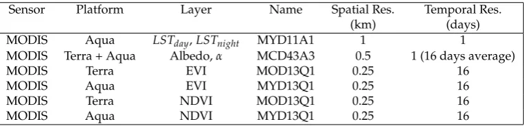
2.2.2. Remote sensing data
The three environmental variables used as predictors in this work (albedo, vegetation index
and surface temperature) were obtained from different MODIS products (Table 1). The R packages
MODIStsp [27] package was used to download and process the images.
The 8 day delay between the MOD13Q1 and MYD13Q1 products allowed combined layers
(AQUA and TERRA satellites) of NDVI and EVI to be obtained, with a temporal resolution of 8 days.
The process involves 3 steps: 1) Elimination of pixels of very low quality or with large observation
Table 1.Main characteristics of MODIS products used in this work
Sensor Platform Layer Name Spatial Res. Temporal Res.
(km) (days)
MODIS Aqua LSTday,LSTnight MYD11A1 1 1
MODIS Terra + Aqua Albedo,α MCD43A3 0.5 1 (16 days average)
MODIS Terra EVI MOD13Q1 0.25 16
MODIS Aqua EVI MYD13Q1 0.25 16
MODIS Terra NDVI MOD13Q1 0.25 16
MODIS Aqua NDVI MYD13Q1 0.25 16
(VIUI) [29,30] were considered to be of very low quality or to have large observation errors, and were
therefore removed. 2) Combining the NDVI/EVI layers. Each layer of NDVI/EVI with an 8-day time
resolution was obtained by combining the layers obtained by the MOD13Q1 and MYD13Q1 products
representing each 8-day period. In this step, therefore, NDVI/EVI values were only obtained from
those pixels in which the values of both products were available. 3) Reconstruction of the existing
gaps after step 2. For this purpose, the average of both layers was used preferably, if the NDVI/EVI
values obtained one week before and one week after were available. Otherwise, the values estimated
one week earlier or later were used. When there were no NDVI/EVI values a week before or after, the
same process were carried out with the estimated values for 2 weeks before and after.
With regard to the LST layers, it was decided to use those provided by the product MYD11A1,
since AQUA passage time is closer than TERRA’s to the temperature recording time. The LST layers
were corrected taking into account the quality of the different pixels. In this case, according to [31] the
LST pixels with an error estimation of more than 3 degrees Kelvin were removed. The GRASS module
i.modis. qcwas used to obtain the error layers.
We assumed, according to [32], that the albedo layers are equal to the 20th layer (White-Sky
Albedo) of the product MCD43A3. In this case, the reconstruction of the existing gaps was carried
out using estimations for the layers 8 days before or after the layer being reconstructed. Within this
interval, the values closest to the existing gap were used.
2.2.3. Geographical variables
The geographical variables used as predictors with the regression methods were
calculated from the official 25 m resolution Digital Elevation Model downloaded from
the Spanish National Geographical Institute (Instituto Geográfcio Nacional, IGN) website
(http://centrodedescargas.cnig.es/CentroDescargas/index.jsp). This MDE was also used to obtain
2.3. Estimation methods
Five methods were used to estimate air temperature at the satellite passage time: TVX is a
well-known method based solely on satellite data; Multiple linear regression, SVM and RF are
regression (global interpolation) methods that rely on covariates to estimate the dependent variable;
in this paper, only covariates that can be easily obtained from a DEM were used, the first based on
classical statistics and the last two on machine learning; finally Ordinary kriging, a local interpolation
method that does not take into account covariates, was used for comparison. Finally, the residuals of
the three regression models were interpolated with OK to obtain regression-kriging models.
2.3.1. The temperature-vegetation index (TVX) method
TVX is based on two hypotheses: 1) linear relation between NDVI and LST (equation2) and
2)Ta = LSTunder full vegetation cover [2,22] while bare soils are significantly hotter in the same
meteorological conditions [22]. It also assumes uniform soil moisture and atmospheric conditions [33].
The first assumption is achieved by using close pixels in a 7x7 window to perform the regression in
equation 3 [34], and the second by only using TVX on clear days [5].
Ta=ai+bi·NDV Imax (2)
There are, however, several other limitations: the LST/NDVI ratio is reduced when there are
differences in sun illumination caused by topography [22], and all cells in the 7x7 window should be
of similar height to prevent temperature variations due to differences in height from adding noise to
the LST/NDVI relation [22]. The method works better when a large range of NDVI is present in the
7x7 window; however, soil moisture should be fairly constant. This can be problematic in agricultural
areas where irrigated and non-irrigated areas are spatially mixed. Moreover, it is also assumed that
there are no differences in aerodynamic resistance within the moving window due to different surface
types [33]. Also, in accordance with [22], sparse vegetation regions show a great uncertainty when
using TVX.
According to [19], TVX does not take into account other factors, such as latitude, longitude,
elevation or julian day, among others, that may affect the relation between LST andTa. Interestingly,
these are the factors usually taken into account in multivariate regressions. Higher residuals have
been reported in winter than in other months [21], which have been attributed to the presence of snow,
although this is not usually a problem in our study area.
The coefficientsai andbi in equation 2are obtained cell by cell calibrating a linear regresion
assumes uniform atmospheric forcing and similar soil moisture conditions in all the cells used to
calibrate. A 7x7 window around each cell is used to approach this assumptions [5,34].
LST=ai+bi·NDV I (3)
As a result of this first step, layers ofaandbare obtained. To obtain the value of NDV Imax(a
single value for the whole study area) we used the technique proposed by [3] and also used by [5]. A
new linear model is calibrated (equation4) with data from weather observations ofTa. In this case,
NDV Imaxis the parameter to calibrate.
Ta−ai =bi·NDV Imax (4)
The parameter NDV Imax varies among different study areas and sensors [3,34]. Prihodko &
Goward [2] derived aNDV Imaxof 0.86 for AVHRR images, while [22] reduced it to 0.7 and [33] to 0.65
using SEVIRI images in the Senegal river basin.[2] even stated thatNDV Imaxcan vary among different
vegetation covers.
A new GRASS module is programmed to calibrate a linear model from two input layers
(independent and dependent) in windows of NxN cells. This produces 3 output layers: containing the
coefficients of the regression and theR2value.
r.neighbors.lm independent=NDVI dependent=LST size=7 a=TVXa b=TVXb r2=TVXr2
Onceai andbi are available, both layers are read in R as well as the weather station data to
calibrate equation4in order to obtainNDV Imax. Finally r.mapcalc is used to apply equation 2 in order
to obtainTa:
r.mapcalc "Ta=TVXa + TVXb * NDVImax"
Our study area has some of the problems that, according to the literature, may reduce the
effectiveness of the model: large variability of land uses in small areas, especially taking into account
the MODIS resolution, sparse vegetation due to semiarid conditions, and frequent cloudiness due to
proximity to the sea.
2.3.2. Multiple Linear regression
Simple and multiple linear regression models (MRLM) are the most popular models for estimating
air temperature. MRLM is a global interpolation method in which a functional relationship is
defined between the dependent variable (in this case maximum and minimum temperature estimated
in different observatories in the territory), and a set of spatially distributed environmental and
generalized least squares (GLS), a modification of OLS that takes into account the heterocedasticity
and the spatial correlation in the observations. In this work, we used the implementation of GLS in the
R package nlme [35].
The assumptions of the model were assessed by hypothesis contrasts: the Kolmogorov-Smirnov
test to assess the normality of residuals (usually met) and the Breush-Pagan test to assess
homocedasticity (usually not met).
With all the regression methods, a first step of variable selection was carried out using the
Variance Inflation Factor (VIF) methodology proposed by [36]. In the case of multiple linear regresssion
a subsequent stepwise procedure was carried out to minimize the number of variables to provide a
more parsimonious model.
2.3.3. Support Vector Machine
SVM was originally developed for classification but it was adapted to regression as a robust
regression method that tries to minimise the effect of outliers. SVM for regression is described in [37].
Instead of trying to minimise the sum of squared errors, data points whose residual absolute values
are lower than a user defined threshold (e) do not contribute to the fit, whereas points with|e| >e
contribute linearly rather than quadratically to the error objective function to be minimized. This
somewhat counterintuitive approach (the more accurately predicted points are not used to fit the line)
has proven effective. SVM is calibrated by minimizing equation5[38].
J=C
N
∑
i=1(ξ+i +ξ−i ) + ||w|| 2
2 (5)
whereCis a cost parameter to penalise large residuals. The solution of equation 5 is also subject
to the following linear constraints:
yi ≤ f(xi) +e+ξi+ (6)
yi ≥ f(xi)−e−ξi− (7)
ξ+i ≥0 (8)
ξ−i ≥0 (9)
(10)
w
∑
i
αi·xi (11)
The estimation of new cases (u) is made with the equation:
ˆ
y=β0+ n
∑
i=1αi·K(xi,u) (12)
whereK(xi,u)is a kernel function,xirepresent each case in the training data andurepresents
predicted values in the new point. There are several possible kernel functions:
• Linear kernel:K(xi,u) =x0i·u
• Radial kernel:K(xi,u) =exp(−σ·(xi·u)2)
• Polynomial kernel:K(xi,u) = (φ(x0i·u) +1)d
• Hyperbolic tangent kernel:K(xi,u) =tanh(φ(xi0·u) +1)
The last three kernels allow a non-linear generalizaton of SVM.
In accordance with equation12, there is anαvalue for each data point. This over-parametrization
is only apparent becauseαi = 0 for all points where |ei| < e; the others are the so-called Support
Vectors.
SVM has been reported to obtain similar accuracy than RF and better accuracy than other machine
learning methods such as neural networks; however, its main drawback is that there is no way to know
in advance which kernel and parameter values will give the best results. In this case, we reduced the
problem by using a radial basis function (RBF) kernel using the default values for the parameters. The
implementation used was that of the R package e1071 [39].
2.3.4. Random Forest
RF is an ensemble of decision trees. In a regression decision tree, heterogeneity of a sample of
training data is measured as the variance of the dependent variable. For a set of samples, the weighted
average of the variances is used. Decision tree algorithm begin with the whole sample and select the
independent variable and its threshold value, which minimise heterogeneity in the resulting partition.
The process continues recursively until a minimum number of cases is reached in all partitions. Each
partition is called a node, and the final partitions are called final nodes. The estimated value of the
dependent variable in each of the final nodes is the average of all cases inside it.
Once the tree is calibrated, the dependent variable for a new case can be estimated by driving the
case through the regression tree until a final node is reached. The previously calculated average for
Decision trees are characterised by a small bias but a high variance. RF tries to solve this issue by
training several (500 as default) decision trees. Each tree is trained with a bootstrapped subsample
of the available training cases (the so-called in-bag cases). In addition, every time a variable has to
be selected to split a node, only a subset of the independent variables is considered (by default the
integer part of√pwherepis the number of variables). In this way, although each tree provides a high
variance estimation, averaging the results of all of them will result in a low bias and low variance
estimation.
RF has 4 main advantages over other machine learning methods: 1) It provides an internal
cross-validation procedure, 2) the default values for the parameters provide optimal estimations most
of the times, 3) The decrease in heterogeneity provided by each variable along the calibration process
of each tree, when aggregated, provides a measure of the importance of each variable, 4) it is possible
to obtain an estimation of the effects of the different predictors on the model, allowing the operator to
decide if such effects are physically sound or not. Points 3 and 4 mean that RF is not really a black box
model, as other ML techniques; rather it might be considered a grey box model.
In this work, we used the version in the R ranger package [40], a very fast and memory efficient
implementation of RF. We used the default values for the ntree (500) and mttry (f loor(√p)) where p is
the number of predictors. Previous research [41,42] has shown that the accuracy achieved with such
parameters is usually near the optimum.
2.3.5. Ordinary kriging
Ordinary kriging is a local interpolation method based on the regionalized variable theory [43]. It
uses solely the values measured in the observation points and their location. Its main advantage over
other local interpolation methods (such as IDW) is that a statistical analysis of the spatial variability of
the values is previously performed and summarised in the semivariogram function. Finally, ordinary
kriging performs, at each pixel, a weighted average of the values in the surrounding observation
points with the weights calculated as a function of the semivariogram. The assumptions of ordinary
kriging are normality and first and second order stationarity, that is, the mean and the variance are
constant in the area. These assumptions are rarely met, so several variations have been proposed to
deal with trends in the data: e.g. universal kriging (taking into account spatial trends in the values)
and regression-kriging (taking into account other covariates).
In this work, we used the R package automap [44], its main advantage being the automatization
of a weighted least squares optimal estimation of semivariogram parameters using Gauss-Newton
2.3.6. Validation
As the aim of this work is to evaluate the predictive performance of the different models, a
leave-one-out cross validation (LOOCV) was carried out for the 8 estimation methods. Bennett et al.
[46] state that Goodness of fit statistics measure different performance aspects, so several statistics
should be used to decide which is the most accurate model. Four statistics, whose detailed description
and interpretation criteria can be consulted in [47] or [46], were used in this research:
Root mean square deviation (RMSE):
RMSE=
r ∑n
i=1(Oi−Ei)2
n (13)
Correlation coefficient:
R= COV(O,E)
sO·sE
(14)
The modified Nash-Sutcliffe efficiency (nse) measures the relative magnitude of the residual
variance compared to the observed data variance, it is less sensitive than R2to outliers [47]:
nse= ∑
n
i=1(Oi−Ei)2
∑n
i=1(Oi−O¯)2
(15)
Percent bias (PBIAS) measures the relative tendency of the estimated values to differ from the
observed values. It is less sensitive than RMSE to outliers and to the magnitude of the data:
PBI AS= ∑
n
i=1(Oi−Ei)
∑n i=1Oi
(16)
The four statistics were calculated each day, so statistical distributions of their values along the
year can be obtained and compared. An alternative option would have been to calculate statistics for
each observatory; however, the temperature variations along the year would produce high r2and NSE
values even if the accuracies of the different observatories were small (Simpson paradox).
As normality and homocedasticity could not be assumed, a Kruskal Wallis contrast was used to
test whether differences among the methods were significant. If that was the case, a post-hoc contrast
between pairs of models, based on Mann-Whitney and using Holm method to correct p-values among
classes, was performed to discover groups of non-significantly different methods.
3. Results and discussion
When TVX was calculated for the 2012 data, the results were disappointing. Figure2shows
coefficients of the regression model; the map in the upper right shows the b parameter (slope) of such
model; and the map in the lower left shows the intercept of the model (Ta when NDVI=0). Although
most slopes were negative, there was a large group of positive ones that were not expected. Although
there is a considerable amount of speckle in the maps, there is also a pattern showing negative slopes
in the higher, more forested areas, and positive in the cultivated areas. The agricultural pattern in the
study area is characterised by small patches due both to the complex topographical patterns and to the
predominance of small properties. This patchiness might be affecting the regression models calibrated
in the 7x7 windows, producing abnormal results.
Finally, the map in the lower right shows the resulting Ta map for May 25, 2012. The map shows a
very convincing pattern, with lower temperature in the highest areas and higher temperature values in
the plains. However, there is a wide variability with completely unrealistic maximum and minimum
values, although the frequency of such values was quite low.
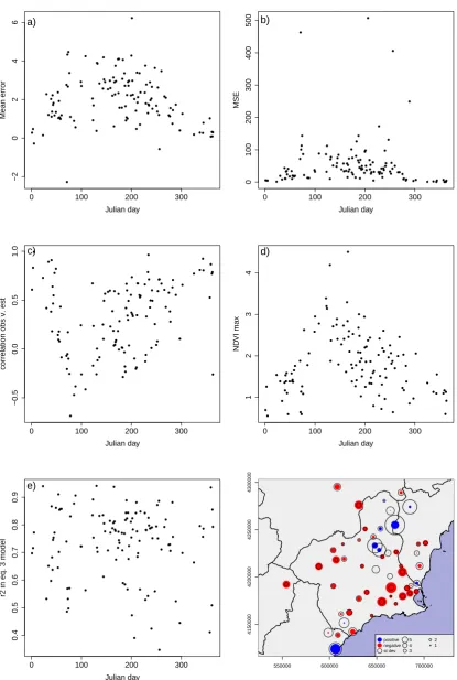
Figure3shows an analysis of the TVX errors through space and time. The first thing to notice is
the high mean error (Figure3a) with a large overestimation of temperature, although it is reduced
on winter days. Mean square errors (Figure3b) are quite high and also tend to be higher in spring.
The correlation between observation and estimation (Figure3c) also shows very abnormal values,
especially on spring days. NDVImax (Figure3d) is too high, with most of the values above 1, which is
clearly an artifact produced by the problems involved in calibrating the focal linear regression in 7x7
windows. However, the temporal pattern is consistent, with the largest values in spring. We tried to
restrict NDVImax beyond 0 and 1, but the errors increased considerably. Despite the high values of
NDVImax , the r2of equation 3 (Figure3e) seems rather high and with no temporal pattern. Finally,
plot f in Figure3shows the spatial pattern of errors. Positive errors (overestimations) are represented
in red and negative errors (underestimations) are represented in blue. The size of the dots represents
the absolute value of the error. The black circles represent the standard deviation of the errors. Most of
the underestimations appear concentrated in the same areas, but it is difficult to deduce a pattern in
relation with other covariates.
We attribute these poor results to the problems associated with the TVX methods. These have
been highlighted in the literature and are indeed present in the study area: sparse vegetation, strong
land use variability at short distances, and also strong topographical variability at short distances.
For the regression models (GLS, RF, SVM) a VIF analysis was previously performed to recursively
eliminate those variables with a high linear correlation with the rest. A threshold of VIF=5 was
stablished in principle, but it was relaxed to allow the inclusion of LST (VIF=6.43). The variables finally
Figure 2.TVX regression parameters on day 145 (May 25) in 2012. Solid lines represent DHS boundaries and dotted lines province boundaries.
Table 2.Mean, standard error and standard deviation of the four validation statistics calculated for the eight temperature estimation methods
GLS RF SVM GLSRK RFRK SVMRK OK TVX
● ● ● ● ● ● ● ● ● ● ●● ● ● ● ● ● ●●● ● ● ● ● ● ● ● ● ● ● ● ● ● ● ● ● ●● ● ● ● ● ● ● ● ● ● ● ● ● ● ● ● ● ● ● ●● ● ● ● ● ● ● ● ● ● ● ● ● ● ● ● ● ● ● ● ● ● ● ● ● ● ● ● ● ● ● ● ●● ● ●● ● ● ● ● ● ● ● ● ● ●● ●● ● ● ● ● ● ● ● ● ● ● ● ● ● ● ●
0 100 200 300
−2 0 2 4 6 Julian day Mean error a) ●●● ● ● ● ● ●● ●● ● ● ● ● ● ●●●● ● ● ● ● ● ● ● ●● ●● ● ● ● ● ● ●● ● ●● ●● ● ● ●● ● ● ● ● ● ● ● ● ● ● ● ● ● ● ● ● ● ● ● ● ● ● ● ● ●● ● ● ● ● ● ● ●● ● ● ● ● ● ●● ● ● ● ●● ● ●● ● ● ● ● ● ● ● ●● ● ● ●●● ● ●● ● ● ●● ● ●●●●
0 100 200 300
0 100 200 300 400 500 Julian day MSE b) ● ● ● ● ● ● ● ● ● ● ● ● ● ● ● ● ● ● ● ●● ● ● ● ● ● ● ● ● ● ● ● ● ● ● ● ● ● ● ● ● ● ●●● ● ● ● ● ● ● ●● ● ● ● ● ●● ● ● ● ● ● ● ● ● ● ● ● ● ● ● ● ● ● ●● ● ●● ● ● ● ● ● ● ● ● ● ● ● ● ● ● ● ● ● ● ● ● ● ● ● ● ● ● ● ● ● ● ● ● ● ● ● ● ● ● ●● ●
0 100 200 300
−0.5
0.0
0.5
1.0
Julian day
correlation obs v. est
c) ● ● ● ● ● ● ● ● ● ● ● ● ● ● ● ● ● ● ● ● ● ● ● ● ● ● ● ● ● ● ● ● ● ● ● ● ● ● ●● ● ● ● ● ● ● ● ● ● ● ● ● ● ● ● ● ● ● ● ● ● ● ● ● ● ● ● ● ● ● ● ● ● ● ● ● ● ● ● ● ● ● ● ● ● ● ● ● ● ● ● ● ● ● ● ● ● ● ● ●● ● ● ● ● ● ● ● ● ● ● ● ● ● ● ● ● ●● ● ● ●
0 100 200 300
1 2 3 4 Julian day ND VI max d) ● ● ● ● ● ● ● ● ● ● ●● ● ● ● ● ● ●●● ● ● ● ● ● ● ● ● ● ●● ● ● ● ● ● ● ● ● ● ● ● ● ● ● ● ● ● ● ● ● ● ● ● ● ● ● ● ● ● ● ● ● ● ● ● ● ● ● ● ● ● ● ● ● ● ● ● ● ●● ● ● ● ● ● ●● ● ● ● ●● ● ● ● ● ● ● ● ● ● ● ● ● ●● ● ● ● ● ● ● ● ● ● ● ● ● ● ● ●
0 100 200 300
0.4 0.5 0.6 0.7 0.8 0.9 Julian day
r2 in eq. 3 model
e)
550000 600000 650000 700000
4150000 4200000 4250000 4300000 ● ● ● ● ●
●
● ● ● ● ● ● ● ● ●●
● ● ● ● ● ● ● ● ● ● ●●
● ● ● ● ● ●●
● ● ● ● ●●
●● ● ● ● ● ● ● ● ● ● ● ●●
● ●●
● ● ● ● ● ●●
● ● ● ● ● ● ● ● ● ● ● ● ● ● ● ● ● ● ● ● ● ● ● ● ● ● ● ● ● ● ● ● ● ● ● ● ● ● ● ● ● ● ● positive negative st dev 5 4 3 2 1● ● ● ● ● ● ● ● ● ● ● ● ● ●
bc ab c bc a bc bc d
0.0 0.3 0.6 0.9
GLS RF SVM GLSRK RFRK SVMRK OK TVX
(a) R2 ● ● ● ● ● ● ● ● ● ● ● ● ● ● ● ● ● ● ● ● ● ● ● ● ● ● ● ● ● ● ● ● ● ● ● ● ● ● ● ● ● ● ● ● ● ●
bc bc bc ab a c bc d
−2 −1 0 1
GLS GLSRK OK RF RFRK SVM SVMRK TVX
(b) NSE ● ● ● ● ● ● ● ● ● ● ● ● ● ● ● ● ● ● ● ● ● ● ● ● ● ● ● ● ● ● ● ● ● ● ● ● ● ● ● ● ●
d b cd d a bc bc e
0 2 4 6
GLS RF SVM GLSRK RFRK SVMRK OK TVX
(c) RMSE (mm)
● ● ● ● ● ● ● ● ● ● ● ● ● ● ● ● ● ● ● ● ● ● ● ● ● ● ● ● ● ● ● ● ● ● ● ● ● ● ● ● ● ● ● ● ● ● ● ● ● ● ● ● ● ● ● ● ● ● ● ● ● ● ● ● ● ● ● ● ● ● ● ● ● ● ● ● ● ● ●
bc c ac a ab ab a d
−2 −1 0 1 2
GLS GLSRK OK RF RFRK SVM SVMRK TVX
(d) PBIAS (%)
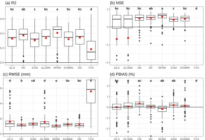
Figure 4. Boxplot showing Anova results of the 4 validation statistics calculated for the eight temperature estimation methods
Table2and Figure4show the results of the cross-validation of the eight methods. The number
of days were 121 with RF, RFRK, SVM, SVMRK and OK, 118 with GLS and GLSRK and 109 for
TVX. The cross validation was limited to those days in which the number of observations (weather
stations without clouds and with data available for that day) was greater than the number of covariates
(10). That means 121 days including 3995 predictions. However, in the case of GLS and GLSRK ,
the final set of predictions was 3928 and 118 days due to errors derived from the estimation of the
variance-covariance matrix. Finally, in the case of TVX, the regression in 7x7 windows extends the need
for cloudless cells to the surroundings of the weather stations, diminishing the number of complete
cases to 1175 predictions on 109 days.
In addition, TVX, GLS and GLSRK show very high prediction errors, although predictions with
absolute residuals larger than 20oC were filtered out. When this filtering was carried out, the final
number was 3886 in the GLS and GLSRK models and 1159 with TVX.
The ANOVA shows significant differences among the algorithms for all the statistics with large F
values (r2: 18.907, NSE: 17.053, RMSE: 67.698, PBIAS: 26.847) and p-values lower than 0.0001 in all
cases. Table2and Figure4show detailed results of such an analysis. The letters above the plots in
figure4indicate to which groups of non-significantly different values belong each method. According
the other methods. According to r2RFRK is still the best method, but its results are not significantly
different from those of RF without residual kriging. Several methods (all except GLS, GLSRK and
TVX) obtain PBIAS values near to zero without being significantly different. On the other hand, for
all statistics TVX produces significantly less accurate results than the other methods. The r2values
obtained by the regression models were very high when measured in calibration (GLS: 0.9165, RF:
0.9939 and SVM: 0.9627).
The bad results of TVX can be explained bt the fact that it only uses satellite data and also because
the conditions in the study area are not adequate for the use of this method. The main advantage of
regression methods, as used in this study, is that only predictors that are easily calculated from MODIS
or conventional MDEs were used. It is also easy to implement in other areas.
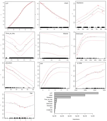
Figure5shows the importance of the predictors and their effects on the model. The most important
predictors are LST, cdayt and radiation. The effect of all of them are clearly as expected, except the
slight reduction in estimated temperature for the largest radiation values. We think the real behaviour
might be a stabilisation of temperature for high radiation, although this was altered because of the
three points with larger temperature estimation, which may represent a local effect. The least important
predictors also have sound effects, although in two of them (Albedo and TWI) confidence intervals are
too large to draw any clear conclusion.
Figure6shows the resulting temperature maps at the satellite passage time for the eight methods
analysed. Due to the strong overestimation of Ta by TVX, a different colour palette is used in the
TVX map. The spatial patterns produced by OK and TVX are clearly poorer as the latter do not use
any ancillary data and the former uses only NDVI and LST. The patterns produced by the regression
methods are quite similar, reproducing the influence of the topographical variables that are relevant
for the modelling of the spatial variability of temperature. The main differences among the regression
methods involves the prediction of maxima and minima. The regression trees on which RF is based
prevent the prediction of abnormally high or low values when the values of the predictors exceed
the values used in calibration. This does not happen with GLS or SVM, whose maps show higher
extremes, especially in the case of the GLS model. These extreme values are, however, smoothed by
the kriging of the residuals. Although the lack of extrapolation is probably a point in favour of RF, it is
difficult to ascertain to what extent it may result in an overestimation of minima and underestimation
of maxima. Finally, all regression methods produce an artifact in the cells nearest the coast, which
10 20 30 40 50 18 20 22 24 26 28 30 y^ ● ● ● ● ● ● ●● ● ● ● ● ● ● ● ● ● ● ● ●● ●●● ●
−1.0 −0.5 0.0 0.5 1.0
20 22 24 26 28 y^ ●● ●● ● ● ●● ● ●● ● ● ● ● ● ● ●● ●● ● ● ● ●
3000 4000 5000 6000 7000 8000 9000
24 .5 25 .0 25 .5 26 .0 y^ ● ● ●● ● ● ● ● ● ●●● ● ● ●● ● ● ● ● ●● ●●●
12.0 12.5 13.0 13.5 14.0
24 .8 25 .0 25 .2 25 .4 25 .6 25 .8 y^ ● ● ● ● ●● ● ● ● ●● ●●●● ● ● ● ●●● ● ● ● ●
0.15 0.20 0.25 0.30
25 .0 25 .1 25 .2 25 .3 25 .4 25 .5 25 .6 y^ ● ● ●●●● ●● ● ●● ●● ●● ● ●●● ●● ● ●● ●
0 20000 40000 60000 80000 100000 120000
24 .5 25 .0 25 .5 26 .0 y^ ●● ●● ● ●● ● ● ●● ● ● ● ●● ●●●● ●●●● ●
0 200 400 600 800 1000
24 .5 25 .0 25 .5 26 .0 y^ elevation ● ● ● ● ●● ● ● ●● ● ●●●● ● ● ● ● ● ● ● ● ● ●
1 2 3 4 5
25 .0 25 .1 25 .2 25 .3 25 .4 25 .5 25 .6 y^ ● ● ● ● ● ● ● ● ● ●●● ●●●●● ●●●●● ● ● ●
0.1 0.2 0.3 0.4 0.5
24 .8 25 .0 25 .2 25 .4 25 .6 25 .8 26 .0 y^ ● ● ● ● ● ● ● ● ● ● ● ●●● ● ●● ● ● ● ● ● ● ● ●
550000 600000 650000 700000
24 .8 25 .0 25 .2 25 .4 25 .6 y^ ● ● ● ●● ●● ● ●● ● ● ● ● ●● ●●●● ● ● ● ● ● X UTM EVI TWI
Time_ps_day Albedo DistCoast LST cdayt Radiation
TWI Longitude EVI Elevation DistCoast Albedo Time_ps_day Radiation cdayt LST Importance
0e+00 2e+04 4e+04 6e+04 8e+04 1e+05
550000 600000 650000 700000
4150000
4200000
4250000
4300000
GLS
550000 600000 650000 700000
4150000
4200000
4250000
4300000
GLS−RK
550000 600000 650000 700000
4150000
4200000
4250000
4300000
SVM
550000 600000 650000 700000
4150000
4200000
4250000
4300000
SVM−RK
550000 600000 650000 700000
4150000
4200000
4250000
4300000
RF
550000 600000 650000 700000
4150000
4200000
4250000
4300000
RF−RK
550000 600000 650000 700000
4150000
4200000
4250000
4300000
OK
550000 600000 650000 700000
4150000
4200000
4250000
4300000
TVX
●
Regression models −6−11.3 11.3−21.2 21.2−23.6 23.6−25.5 25.5−27.1 27.1−28.3 28.3−29.5 29.5−31.1 31.1−33.9 33.9−44.9
TVX −40−14.6 14.6−25.1 25.1−30.7 30.7−34.7 34.7−38.3 38.3−41.6 41.6−45.1 45.1−49.7 49.7−58.7 58.7−144.3
4. Conclusions
Random Forest with ordinary kriging of the residuals obtained the most accurate results with
r2=0.612, SE=0.578, RMSE=1.068 and PBIAS=-0.17. The last result indicates that it is the only method
that produces a slight temperature underestimation, whereas the rest of the methods overestimate
temperature to a greater or lesser degree. The maps obtained with RF do not show the extreme values
usually present in other regression methods, and that also appear in this study. It is interesting to
note that RF obtained more accurate results than SVM, even when the parameters of the latter were
optimized but not those of the former. Finally, TVX was the method that produced the worst results,
probably because the environmental conditions in the study area are not suited to this method and
also because the predictors used by the regression methods explain an important part of temperature
variability.
Author Contributions: Conceptualization, Marcos Ruiz-Álvarez, Francisco Alonso-Sarria and Francisco
Gomariz-Castillo; Investigation, Marcos Ruiz-Álvarez; Methodology, Marcos Ruiz-Álvarez, Francisco
Alonso-Sarria and Francisco Gomariz-Castillo; Project administration, Francisco Alonso-Sarria; Software, Francisco
Alonso-Sarria and Francisco Gomariz-Castillo; Supervision, Francisco Alonso-Sarria; Writing – original draft,
Marcos Ruiz-Álvarez and Francisco Alonso-Sarria; Writing – review & editing, Francisco Alonso-Sarria.
Funding:This research received no external funding.
Acknowledgments:Pensad si quereis meter alguno.
Conflicts of Interest:The authors declare no conflict of interest.
Abbreviations
The following abbreviations are used in this manuscript:
LST Land Surface Temperature
MLRM Multiple Linear Regression Model
OLS Ordinary Least Squares
GLS Generalised Least Squares
RF Random Forest
SVM Support Vector Machine
OK Ordinary Kriging
RK Regression Kriging
VIF Variance Inflation Factor
References
1. Liu, S.; Su, H.; Zhang, R.; Tian, J.; Wang, W. Estimating the Surface Air Temperature by Remote Sensing in Northwest China Using an Improved Advection-Energy Balance for Air Temperature Model.Advances in Meteorology2016, p. 11.
2. Prihodko, L.; Goward, S.N. Estimation of air temperature from remotely sensed surface observations. Remote Sensing of Environment1997,60, 335–346.
3. Nieto, H.; Sandholt, I.; Aguado, I.; Chuvieco, E.; Stisen, E. Air temperature estimation with MSG-SEVIRI data: Calibration and validation of the TVX algorithm for the Iberian Peninsula. Remote Sens. Environ. 2011,115, 107–116.
4. Zhang, R.; Rong, Y.; Tian, J.; Su, H.; Li, Z.L.; Liu, S. A Remote Sensing Method for Estimating Surface Air Temperature and Surface Vapor Pressure on a Regional Scale. Remote Sensing2015,7, 6005–6025. 5. Liu, S.; Su, H.; TIAN, J.; Zhang, R.; Wang, W.; Wu, Y. Evaluating Four Remote Sensing Methods for
Estimating Surface Air Temperature on a Regional Scale. Journal of Applied Meteorology and Climatology 2017,56, 803–814.
6. Zhu, W.; Lu, A.; Jia, S.; Yan, J.; Mahmood, R. Retrievals of all-weather daytime air temperature from MODIS products. Remote Sens. Environ.2017,189, 152–163.
7. Vogt, J.; Viau, A.; Paquet, F. Mapping regional air temperature fields using satellite-derived surface skin temperatures. International Journal of Climatology1997,17, 1559–1579.
8. Cresswell, M.; Morse, A.; Thomson, M.; Connor, S. Estimating surface air temperatures, from Meteosat land surface temperatures, using an empirical solar zenith angle model.Int. J. Remote Sens.1999,20, 1125–1132. 9. Jang, J.; Viau, A.; Anctil, F. Neural network estimation of air temperatures from AVHRR data.Int. J. Remote
Sens.2004,25, 4541–4554.
10. Lin, S.; Moore, N.; Messina, J.; DeVisser, M.; Wu, J. Evaluation of estimating daily maximum and minimum air temperature with MODIS data in east Africa.Int. J. Appl. Earth Obs. Geoinf.2012,18, 128–140. 11. Benali, A.; Carvalho, A.; Nunes, J.; Carvalhais, N.; Santos, A. Estimating Air Surface Temperature in
Portugal Using MODIS LST Data.Remote Sensing of Environment2012,124, 108–121.
12. Kim, D.; Han, K. Remotely Sensed Retrieval of Midday Air Temperature Considering Atmospheric and Surface Moisture Conditions. International Journal of Remote Sensing2013.,34, 247–263.
13. Zakšek, K.; Schroedter-Homscheidt, M. Parameterization of air temperature in high temporal and spatial resolution from a combination of the SEVIRI and MODIS instruments. ISPRS J. Photogramm. Remote Sens. 2009,64, 414–421.
14. Xu, Y.; Knudby, A.; Ho, H.C. Estimating daily maximum air temperature from MODIS in British Columbia, Canada. International Journal of Remote Sensing2014,35, 8108–8121.
15. Cristóbal, J.; Ninyerola, M.; Pons, X. Modeling air temperature through a combination of remote sensing and GIS data.J. Geophys. Res.2008,113, D13106.
16. Fu, G.; Shen, Z.; Zhang, X.; Shi, P.; Zhang, Y.; Wu, J. Estimating air temperature of an alpine meadow on the Northern Tibetan Plateau using MODIS land surface temperature. Acta Ecol. Sin.2011,21, 8–13. 17. Vancutsem, C.; Ceccato, P.; Dinku, T.; Connor, S. Evaluation of MODIS Land Surface Temperature Data to
Estimate Air Temperature in Different Ecosystems over Africa. Remote Sens. Environ.2010,114, 449–465. 18. Kloog, I.; Nordio, F.; Coull, B.; Schwartz, J. Predicting Spatiotemporal Mean Air Temperature Using MODIS
Satellite Surface Temperature Measurements across the Northeastern USA. Remote Sens. Environ.2014, 150, 132–139.
19. Yang, Y.Z.; Cai, W.H.; Yang, J. Evaluation of MODIS Land Surface Temperature Data to Estimate Near-Surface Air Temperature in Northeast China.Remote Sens.2017,9, 410.
20. Nemani, R.R.; Running, S.W. Estimation of regional surface resistance to evapotranspiration from NDVI and thermal-IR AVHRR data.Journal of Applied Meteorology1989,28, 276–284.
21. Goward, S.N.; Waring, R.; Dye, D.; Yang, J. Ecological remote sensing at OTTER: Satellite macroscale observations. Ecological Applications1994,4, 322–343.
22. Czajkowski, K.; Mulhern, T.; Goward, S.; Cihlar, J.; Dubayah, R.; Prince, S. Biospheric environmental monitoring at BOREAS with AVHRR observations. J. Geophys. Res.1997,102, 651–662.
24. Sørensen, R.; Zinko, U.; Seibert, J. On the calculation of the topographic wetness index: evaluation of different methods based on field observations. Hydrology and Earth System Sciences2006,10, 101–112. 25. Hofierka, J.; Suri, M. The solar radiation model for Open source GIS: implementation and applications.
International GRASS users conference, 2002.
26. Gasch, C.; Hengl, T.; Gräler, B.; Meyer, H.; Magney, T.; Brown, D. Spatio-temporal interpolation of soil water, temperature, and electrical conductivity in 3D + T: The Cook Agronomy Farm data set. Spatial Statistics2015,14, 70–90.
27. Busetto, L.; Ranghetti, L. MODIStsp: An R package for automatic preprocessing of MODIS Land Products time series. Computers & Geosciences2016,97, 40–48.
28. Priyadarshi, N.; Chowdary, V.; Srivastava, Y.; Das, I.C.; Jha, C.S. Reconstruction of time series MODIS EVI data using de-noising algorithms. Geocarto International2017, pp. 1–19.
29. Huete, A.; Justice, C.; Van Leeuwen, W. MODIS vegetation index (MOD13). Algorithm theoretical basis document1999,3, 213.
30. Gu, J.; Li, X.; Huang, C.; Okin, G.S. A simplified data assimilation method for reconstructing time-series MODIS NDVI data. Advances in Space Research2009,44, 501–509.
31. Metz, M.; Andreo, V.; Neteler, M. A New Fully Gap-Free Time Series of Land Surface Temperature from MODIS LST Data. Remote Sensing2017,9, 1333.
32. Mu, Q.; Zhao, M.; Running, S.W. Improvements to a MODIS global terrestrial evapotranspiration algorithm. Remote Sensing of Environment2011,115, 1781–1800.
33. Stisen, S.; Sandholt, I.; Nørgaard, A.; Fensholt, R.; Eklundh, L. Estimation of diurnal air temperature using MSG SEVIRI data in West Africa.Remote Sens. Environ.2007,110, 262–274.
34. Zhu, W.; Lu, A.; Jia, S. Estimation of daily maximum and minimum air temperature using MODIS land surface temperature products. Remote Sens. Environ.2013,130, 62–73.
35. Pinheiro, J.; Bates, D.; DebRoy, S.; Sarkar, D.; Team, R.C. nlme: Linear and Nonlinear Mixed Effects Models. Technical report, 2018.
36. Zuur, A.; Ieno, E.; Walker, N.; Saveliev, A.; Smith, G.Mixed Effects Models and Extensions in Ecology with R; Springer, 2009; p. 549.
37. Kuhn, M.; Johnson, K.Applied Predictive Modeling; Springer, 2013.
38. Murphy, K.Machine Learning. A propbabilistic approach; The MIT Press, 2012.
39. Meyer, D.; Dimitriadou, E.; Hornik, K.; Weingessel, A.; Leisch, F. e1071: Misc Functions of the Department of Statistics, Probability Theory Group (Formerly: E1071), TU Wien. Technical report, 2018.
40. Wright, M.N.; Ziegler, A. ranger. A Fast Implementation of Random Forests for High Dimensional Data in C++ and R.Journal of Statistical Software2017,77(1), 1–17.
41. Liaw, A.; Wiener, M. Classification and Regression by randomForest. R News2002,2(3), 18–22.
42. Cánovas-García, F.; Alonso-Sarria, F. Optimal Combination of Classification Algorithms and Feature Ranking Methods for Object-Based Classification of Submeter Resolution Z/I-Imaging DMC Imagery. Remote Sensing2015,74(4), 4651–4677.
43. Burrough, P.; McDonnell, R.; Lloyd, C.Principles of Geographical Information Systems; Oxford, 2015. 44. Hiemstra, P.; Pebesma, E.; Twenhöfel, C.; Heuvelink, G. Real-time automatic interpolation of ambient
gamma dose rates from the Dutch Radioactivity Monitoring Network. Computers & Geosciences2008, 35(8), 1711–1721.
45. Cressie, N.Statistics for Spatial Data (Revised Ed); Wiley, 1993.
46. Bennett, N.D.; Croke, B.F.; Guariso, G.; Guillaume, J.H.; Hamilton, S.H.; Jakeman, A.J.; Marsili-Libelli, S.; Newham, L.T.; Norton, J.P.; Perrin, C.; Pierce, S.A.; Robson, B.; Seppelt, R.; Voinov, A.A.; Fath, B.D.; Andreassian, V. Characterising performance of environmental models.Environmental Modelling & Software 2013,40, 1 – 20.