Applying ANN, ANFIS, and LSSVM Models for Estimation of Acid Solvent Solubility in Supercritical CO

(1)

Applying ANN, ANFIS, and LSSVM Models for Estimation of Acid

Solvent Solubility in Supercritical CO

2

Amin Bemani1, Alireza Baghban2, Shahaboddin Shamshirband3,4,*

1 _{Petroleum engineering department, Petroleum university of technology, Ahwaz, Iran}

2 _{Chemical engineering department, Amirkabir university of technology, Mahshahr Campus,} Mahshahr, Iran

3_{Department for Management of Science and Technology Development, Ton Duc Thang}

University, Ho Chi Minh City, Viet Nam

4_{Faculty of Information Technology, Ton Duc Thang University, Ho Chi Minh City, Viet Nam}

Abstract

In the present work, a novel and the robust computational investigation is carried out to estimate solubility of different acids in supercritical carbon dioxide. Four different algorithms such as radial basis function artificial neural network, Multi-layer Perceptron artificial neural network, Least squares support vector machine and adaptive neuro-fuzzy inference system are developed to predict the solubility of different acids in carbon dioxide based on the temperature, pressure, hydrogen number, carbon number, molecular weight, and acid dissociation constant of acid. In the purpose of best evaluation of proposed models, different graphical and statistical analyses and also a novel sensitivity analysis are carried out. The present study proposed the great manners for best acid solubility estimation in supercritical carbon dioxide, which can be helpful for engineers and chemists to predict operational conditions in industries.

Keywords: Supercritical carbon dioxide, Modeling, Acid, Artificial intelligence, Solubility

*_{Corresponding author}

S.Shamshirband ( [email protected])

(2)

1. Introduction

In the recent years, supercritical fluid has become one of the interests of chemical engineers and

chemists as a novel and extensive applicable technology. The synthesis and generating of

nanomaterials and extraction process of different materials are the popular applications of

supercritical fluids [1-13]. One of the supercritical fluids which have wide applications in the

extraction of various metals from solid and liquid phases [14-16]. Due to non-flammability,

nontoxicity, low cost and critical points (304.2 K and 7.38 MPa) of carbon dioxide, the

supercritical carbon dioxide becomes one the interesting and applicable supercritical fluids in

industries[17, 18]. The viscosity and density of supercritical carbon dioxide are known as two

important transport properties of the fluids which are affected by pressure and temperature.

Another dominant thermos physical property of supercritical carbon dioxide is solubility of

different materials in supercritical carbon dioxide which is a function of various factors such as

polarity, molecular weight, pressure, temperature and vapor pressure[19, 20].

One types of the materials which have a solubility in supercritical carbon dioxide are acids, the

nanofluoropentanoic acid which is known as one type of perfluorocarboxylic acids, has extensive

applications in the production of paints additives, polymers, foams and stain repellents but because

of their high ability instability they are harmful to environment[21-27]. Adrien Dartiguelongue

and coworkers studied solubility of perfluoropentanoic acid in supercritical carbon dioxide in the

wide range of temperature and pressure and also proposed some density based models to predict

solubility in terms of density of supercritical fluids [22]. Gurdial et al. constructed dynamic setup

to study solubility of o-, m- and p-hydroxybenzoic acid in the supercritical carbon dioxide in the

wide range pressure of 80-205 mbar and temperature range of 35-55 C and correlated the measured

(3)

2R,3β-dihydroxyurs-12-en-28-oic acid which is called Corosolic acid dynamically in a different range of pressure 8 to

30 MPa and five different temperatures of 308.15, 313.15, 323.15 and 333.15 K. Kumoro used

various density based models to correlate the experimental data[29].

Sahihi et al. measured the solubility of Maleic acid in supercritical carbon dioxide by utilization

of static experimental setup. The measured data belongs to Maleic acid in pressure range of 7 to

30 MPa and temperature of 348.15 K[30]. Ghaziaskar and coworkers used a continuous flow set

up to study solubility of tracetin, diacentin and acetic acid in supercritical carbon dioxide in the

pressure range of 70 to 180 bar and various temperature of 313, 333 and 348 K and they also

compared the obtained solubilities for different acids[31]. Helena Sovova adjusted the Adachi-Lu

equation based on the solubility of Ribes nigrum (blackcurrant) and Vitis vinifera (grape-vine) in

supercritical carbon dioxide. They concluded the Adachi-Lu equation has enough accuracy in

forecasting solubility of triglycerides in carbon dioxide[32].

The issue of prediction of various acids solubility in supercritical carbon dioxide and phase

equilibrium investigation of supercritical carbon dioxide and different materials are the important

topics in chemical engineering research. According to the hardships of experimental studies such

as special tools and procedure which are needed, in the present work, the mathematical

investigation is considered as a great solution for these problems. In this paper four different

algorithms, Radial basis function artificial neural network (RBF-ANN), Multi-layer Perceptron

artificial neural network (MLP-ANN), Least squares support vector machine (LSSVM) and

Adaptive neuro-fuzzy inference system (ANFIS) are developed to predict the solubility of different

types of acid in supercritical carbon dioxide based on the various parameters such as structure of

(4)

2. Methodology

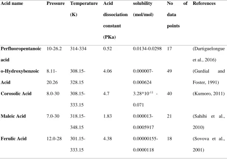
2.1.Experimental Data Gathering

The dominant purpose of present paper is development of accurate and simple models to forecast

solubility of different acids in supercritical carbon dioxide. Due to this, the required actual data for

training and testing phases of models were assembled from the reliable source existed in literature

[22, 28, 29, 32-35]. This collection of data contains the 180 acid solubility data points in terms of

pressure, temperature and different acid structure. The details of data collection are reported in

Table S1. Also, for clarification of this experimental dataset, the structure, linear formula and

molecular weight of utilized acids are presented in Table S2.

Table S1. Experimental data which are used in this study

Acid name Pressure Temperature

(K) Acid dissociation constant (PKa) solubility (mol/mol)

No of

data

points

References

Perfluoropentanoic

acid

10-26.2 314-334 0.52 0.0134-0.0298 17 (Dartiguelongue

et al., 2016)

o-Hydroxybenzoic Acid 8.11-20.26 308.15-328.15

4.06

0.000007-0.000624

49 (Gurdial and

Foster, 1991)

Corosolic Acid 8.0-30

308.15-333.15

4.7 3.28*10-11_- 0.071

40 (Kumoro, 2011)

Maleic Acid 7.0-30

318.15-348.15

1.83

0.000013-0.0005917

21 (Sahihi et al.,

2010)

Ferulic Acid 12.0-28

301.15-333.15

4.38

0.00000155-0.0000118

18 (Sovova et al.,

(5)

Azelaic Acid 10.0-30

313.15-333.15

4.84

0.00000042-0.00001012

14 (Sparks et al.,

2007)

Nonanoic Acid 10.0-30

313.15-333.15

4.96

0.00013-0.00782

14 (Sparks et al.,

2008)

p-aminobanzoic

acid

8.0-21 308-328.0 4.78

0.000001302-0.000006452

15 (Tian et al.,

2007)

Total=188

Table S2. Details of acids which are utilized in this investigation.

Acid name structure Empirical Formula or linear

formula

Molecular

weight

gr/mole

Perfluoropentanoic

acid

CF3(CF2)3COOH 264.05

o-Hydroxybenzoic

Acid

HOC6H4CO2H 138.12

(6)

Maleic Acid HO2CCH=CHCO2H 116.07

Ferulic Acid HOC6H3(OCH3)CH=CHCO2H 194.18

Azelaic Acid HO2C(CH2)7CO2H 188.22

Nonanoic (Sparks

et al., 2008) Acid

CH3(CH2)7COOH 158.24

p-aminobanzoic

acid

C₇H₇NO₂ 137.14

2.2.Artificial neural network

Artificial neural networks have amazing similarities to the performance and structure of neuron

units in the brain system[36, 37]. These computational blocks construct different types of layer

(7)

function which organize the process of training in the algorithm. Each neuron has specific weight

and bias values which control the optimization process. Artificial neural network has ability of

tracing a nonlinear form relationship between input and output parameters. Due to this ability,

artificial neural networks have widespread application in different industries and sciences [38-44].

Artificial neural networks can be classified in different forms such as a recurrent neural network

(RNN), radial basis function and multilayer perceptron [45, 46]. In the present work, the MLP and

RBF network are utilized.

2.3.Least squares support vector machine

Vapnik organized support vector machine based on statistical learning theory[47]. This

computational intelligence can be used for regression and classification purposes. However, there

are many advantages to this method but there is a hardship in its computational procedure because

of quadratic programming. The least squares SVM (LSSVM) is proposed as a novel type of SVM

to solve this problem. This novel approach organized linear equations for computation and

optimization[48-50].

By considering a dataset of (xi,yi)n, the LSSVM regression prediction is utilized to estimate a

function, where xi and yi are known as input and target parameters and n represent the number of

data which utilized in training phase[51]. The linear regression is formulated such as following:

𝑦 = 𝜔𝑇φ(x) + b Eq. (1)

Where φ(x) denotes a nonlinear function that has different forms such as polynomial, linear,

(8)

coefficient in training process. A new optimization problem can be defined based on LSSVM approach[52]: 𝑚𝑖𝑛 𝜔,𝑏,𝑒𝐽 (𝜔, 𝑒) = 1 2𝜔

𝑇_{𝜔 +}1

2𝛾 ∑ 𝑒𝑘

2 𝑁

𝑘=1 Eq. (2)

Which is related to the below constraints:

𝑦_𝑘= 𝜔𝑇_𝜑(𝑥

𝑘) + 𝑏 + 𝑒𝑘 k=1,2,…,N Eq. (3)

The Lagrangian equation is constructed to solve the optimization problem:

L(ω, b, e, α) = 𝐽 (𝜔, 𝑒) − ∑𝑁𝑘=1𝛼𝑘{𝜔𝑇𝜑(𝑥𝑘)+ 𝑏 + 𝑒𝑘− 𝑦𝑘} Eq. (4)

Whereϒ and ek are known as regularization parameter and regression error. The αk represent the

support value. To solve the above problem, the above equation is differentiated with respect to the

different parameters:

𝜕𝐿(ω,b,e,α)

𝜕𝜔 = 0 → 𝜔 = ∑ 𝛼𝑘

𝑁

𝑘=1 𝜑(𝑥𝑘) Eq. (5)

𝜕𝐿(ω,b,e,α)

𝜕𝑏 = 0 → ∑ 𝛼𝑘

𝑁

𝑘=1 = 0 Eq. (6)

𝜕𝐿(ω,b,e,α)

𝜕𝑒𝑘 = 0 → 𝛼𝑘 = 𝛾𝑒𝑘, k=1,2,…,N Eq. (7)

𝜕𝐿(ω,b,e,α)

𝜕𝛼𝑘 = 0 → 𝑦𝑘 = 𝜔

𝑇_𝜑(𝑥

𝑘) + 𝑏 + 𝑒𝑘 k=1,2,…,N Eq. (8)

Karush– Kuhn–Trucker matrix can be obtained by elimination of ω and e[50, 53, 54]:

[0 1𝑣

𝑇

1_𝑣 𝛺 + 𝛾−1_𝐼] [ 𝑏 𝛼] = [

0

(9)

Which 𝑦 = [𝑦₁… 𝑦_𝑁]𝑇_{,𝛼 = [𝛼}

1… 𝛼𝑁]𝑇,1𝑁 = [1 … 1]𝑇 and I represents the identity matrix. 𝛀kl is

𝜑(𝑥_𝑘)𝑇_𝜑(𝑥

𝑙) = 𝐾(𝑥𝑘, 𝑥𝑙). K(xk,xl) is known as kernel function which can be in different forms of

linear, polynomial and radial basis function forms[55]. The estimating function form of LSSVM

algorithm can be expressed as following formulation[56]:

𝑦(𝑥) = ∑𝑁𝑘=1𝛼𝑘𝐾(𝑥, 𝑥𝑘) + 𝑏 Eq. (10)

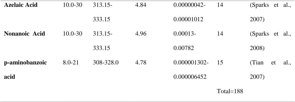
2.4.Adaptive neuro-fuzzy inference system (ANFIS)

Adaptive neuro-fuzzy inference system which is called ANFIS algorithm, in brief, has five

different layers. The aforementioned approach was developed by Jang and Sun[57]. The hybrid

learning approach and back propagation are known as fundamentals of training of conventional

ANFIS algorithm. The ANFIS algorithm was born base on fuzzy logic and neural network

advantages and also the different evolutionary methods such as Imperialist Competitive Algorithm

(ICA), Particle Swarm Optimization (PSO) and Genetic algorithm (GA) can be used to reach the

optimal structure of ANFIS algorithm[38, 40, 58-61]. The ANFIS structure is demonstrated in

(10)

Figure 1: Typical construction of ANFIS approach

In the first layer, the linguistic terms are build base on input data. The Gaussian membership

function is applied to organize these linguistic terms. The Gaussian function can be shown as

following formulation[62]:

𝑂_𝑖1 = 𝛽(𝑋) = 𝑒𝑥𝑝(−

1 2

(𝑋−𝑍)2

𝜎2 )_{Eq. (11)}

Where Z and σ denote the Gaussian parameters.

The next layer contains the weighted terms which are related to rules:

𝑂_𝑖2 = 𝑊_𝑖 = 𝛽_𝐴𝑖(𝑋). 𝛽_𝐵𝑖(𝑋) Eq. (12)

In the third layer the averages of determined weight are determined such as the following

(11)

𝑂_𝑖3 = 𝑊𝑖

∑ 𝑊𝑖 Eq. (13)

Then in the next layer, the average weight values are multiple to the related function such as below:

𝑂_𝑖4 = 𝑊̅̅̅𝑓_𝑖 _𝑖 = 𝑊̅̅̅(𝑚_𝑖 _𝑖𝑋₁+ 𝑛_𝑖𝑋₂ + 𝑟_𝑖) Eq. (14)

Where, m, n, and r represent the resulting indexes.

At last, the fifth layer consists of the summation of previous layer outputs:

𝑂_𝑖5 = 𝑌 = ∑ 𝑊_𝑖̅̅̅𝑓_𝑖 _𝑖 = 𝑊̅̅̅̅𝑓₁ ₁ + 𝑊̅̅̅̅𝑓₂ ₂ =∑ 𝑊𝑖𝑓𝑖

∑ 𝑊𝑖 Eq. (15)

2.5.Particle swarm optimization (PSO)

The combination of random probability distribution approach and generation of the population

constructed the particle swarm optimization algorithm. Eberhart et al. introduced the PSO

algorithm that comes from the social behavior of birds and developed it to solve the nonlinear

function optimization problems[63]. This strategy has special similarities with other optimization

approach such as genetic algorithm which is constructed base on random solution population. Each

particle can be known as a probable solution of problem. A random population of particle created

in search space to relate in optimum system. Pbest is known as the best solution which can obtained

from this strategy for a particle. Also gbest represents the global best solution determined by swarm.

The particle move in the space by time iterations and the next iteration velocity is determined by

using gbest , Pbest and current velocity[64]. The P'th particle can be determined as follow:

𝑋_𝑝𝑑𝑖𝑡𝑒𝑟+1 = 𝑋_𝑝𝑑𝑖𝑡𝑒𝑟+ 𝑉_𝑝𝑑𝑖𝑡𝑒𝑟+1 Eq. (16)

(12)

𝑣𝑖𝑑(𝑡 + 1) = 𝑤𝑣𝑖𝑑(𝑡) + 𝑐1𝑟1(𝑝𝑏𝑒𝑠𝑡,𝑖𝑑(𝑡) − 𝑋𝑖𝑖𝑑(𝑡)) + 𝑐2𝑟2(𝑔𝑏𝑒𝑠𝑡,𝑑(𝑡) − 𝑋𝑖𝑑(𝑡)) Eq. (17)

w, c, and r are inertia weight, learning rate and random number respectively[65-69].

3. Results and discussion

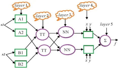
In the present study, the determined structure of MLP-ANN algorithm utilizes log-sigmoid and

linear activation functions the hidden and output layers respectively. By utilization of trial and

error, the optimum number of neurons in hidden layers is determined as 7 to reach the best structure

of MLP-ANN algorithm. The performance of Levenberg Marquardt training of MLP-ANN

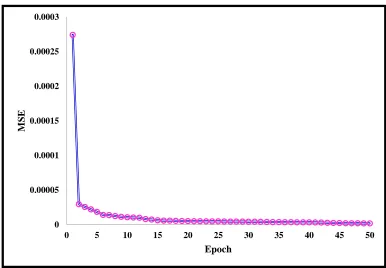
algorithm based on the mean square error is shown in Figure 2. In the RBF-ANN algorithm, the

radial basis function (RBF) is utilized for hidden layers. According to information in the literature,

the hidden layer neurons for RBF-ANN can be supposed one-tenth of training data points. The

training process of RBF-ANN algorithm base on MSE has been reported in Figure 3. In this work,

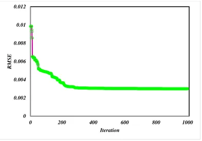
particle swarm optimization approach is applied to train the best structure of ANFIS algorithm.

Figure 4 demonstrates the gained root mean squared error (RMSE) of estimated and experimental

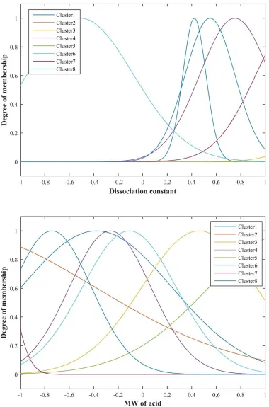
acid solubility values in training step. The optimum structure of ANFIS can be recognized by the

RMSE value of 0.003 after 1000 of iteration steps. Trained membership functions of proposed

(13)

Figure 2: Trained MLP-ANN model by Levenberg Marquardt algorithm

Figure 3: Trained RBF-ANN approach by Levenberg Marquardt algorithm

0 0.00005 0.0001 0.00015 0.0002 0.00025 0.0003

0 5 10 15 20 25 30 35 40 45 50

M

SE

(14)

Figure 4: Performance of trained ANFIS model

0 0.002 0.004 0.006 0.008 0.01 0.012

0 200 400 600 800 1000

R

MSE

(15)

(16)

(17)

(18)

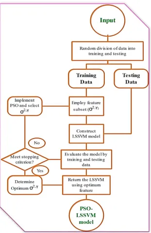
The RBF kernel function due to its high degree of performance is utilized to construct the LSSVM

algorithm. The LSSVM algorithm has two tuning parameters, σ2_and_ϒ_{which are determined by}

utilizing PSO algorithm. The schematic demonstration of LSSVM algorithm is depicted in Figure 6. The details of predicting models are summarized in Table 1.

(19)

Table 1: Details of proposed models

Type comment/value Type comment/value

LSSVM ANFIS

Kernel function RBF Membership function Gaussian

σ2 _0.80321 _No. _of _membership _function

parameters

112

ϒ 12893.2264 No. of clusters 8

Number of data utilized for training

141 Number of data utilized for training 141

Number of data utilized for testing

47 Number of data utilized for testing 47

Population size 85 Population size 50

Iteration 1000 Iteration 1000

C1 1 C1 1

C2 2 C2 2

MLP-ANN MLP-ANN

No. input neuron layer 6 No. input neuron layer 6

No. hidden neuron layer 8 No. hidden neuron layer 50

No. output neuron layer 1 No. output neuron layer 1

Hidden layer activation function

Sigmoid Hidden layer activation function RBF

output layer activation function

linear output layer activation function linear

Number of data utilized for training

141 Number of data utilized for training 141

Number of data utilized for testing

47 Number of data utilized for testing 47

Number of max iteration 1500 Number of max iteration 50

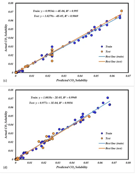
In order to show the performance of proposed models in prediction of solubility of different acids,

regression plots of RBF-ANN, MLP-ANN, ANFIS and LSSVM algorithms are depicted in Figure 7 to compare the determined and actual solubility values. Based on these plots, the surprising fits

for the predicting algorithms are obtained. Also, the predicted acid solubility data for proposed

models are demonstrated along with the corresponding actual acid solubility values in Figure S1.

It can be observed that the model's output solubility values have excellent agreement with actual

solubility values. Another graphical evaluation method is a demonstration of relative error between

(20)

percentage of absolute error for the different predicting algorithm, which expresses the acceptable

degree of accuracy in prediction of acid solubility.

Train: y = 1.005x + 1E-05, R² = 0.9993

Test: y = 0.9903x - 2E-05, R² = 0.9982

0 0.01 0.02 0.03 0.04 0.05 0.06 0.07 0.08

A ctua l CO 2 So lub ilit y

Predicted CO₂Solubility

Train

Test

Best line (train)

Best line (test)

(a)

Test: y = 1.0113x - 0.0001, R² = 0.9654

Train: y = 0.9597x + 0.0004, R² = 0.975

0 0.01 0.02 0.03 0.04 0.05 0.06 0.07 0.08

Train

Test

(21)

Figure 7: Regression plots obtained for different models Train: y = 0.9934x + 4E-06, R² = 0.995

Test: y = 1.0279x - 4E-05, R² = 0.9869

0 0.01 0.02 0.03 0.04 0.05 0.06 0.07 0.08

0 0.01 0.02 0.03 0.04 0.05 0.06 0.07

Predicted CO2 Solubility

Train

Test

(c)

Train: y = 1.0038x - 2E-05, R² = 0.9948

Test: y = 0.977x + 1E-04, R² = 0.9856

0 0.01 0.02 0.03 0.04 0.05 0.06 0.07 0.08

Train

Test

(22)

0 0.01 0.02 0.03 0.04 0.05 0.06 0.07 0.08

0 20 40 60 80 100 120 140 160 180 200

CO

2

So

lub

ilit

y

Data Index

Train Exp. Test Exp. Train LSSVM Test LSSVM

0 0.01 0.02 0.03 0.04 0.05 0.06 0.07 0.08

0 20 40 60 80 100 120 140 160 180 200

CO

2

So

lub

ilit

y

Data Index

(23)

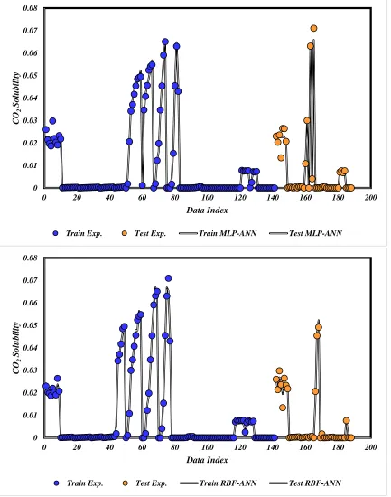
Figure S1: Experimental and predicted solubility of CO2 by the proposed models 0

0.01 0.02 0.03 0.04 0.05 0.06 0.07 0.08

0 20 40 60 80 100 120 140 160 180 200

CO

2

So

lub

ilit

y

Data Index

Train Exp. Test Exp. Train MLP-ANN Test MLP-ANN

0 0.01 0.02 0.03 0.04 0.05 0.06 0.07 0.08

0 20 40 60 80 100 120 140 160 180 200

CO

2

So

lub

ilit

y

Data Index

(24)

-0.5 -0.4 -0.3 -0.2 -0.1 0 0.1 0.2 0.3 0.4

0 0.01 0.02 0.03 0.04 0.05 0.06 0.07 0.08

A b so lut e Dev ia tio n ( % )

CO₂Solubility

Train Test (a) -2 -1.5 -1 -0.5 0 0.5 1 1.5 2

0 0.01 0.02 0.03 0.04 0.05 0.06 0.07 0.08

CO₂Solubility

Train Test

(25)

Figure S2: Absolut deviation plots for (a) LSSVM, (b) ANFIS, (c) MLP-ANN, and (d) RBF-ANN -1.2 -1 -0.8 -0.6 -0.4 -0.2 0 0.2 0.4 0.6 0.8

0 0.01 0.02 0.03 0.04 0.05 0.06 0.07 0.08

CO₂Solubility

Train Test (c) -0.8 -0.6 -0.4 -0.2 0 0.2 0.4 0.6 0.8

0 0.01 0.02 0.03 0.04 0.05 0.06 0.07 0.08

CO₂Solubility

Train Test

(26)

Furthermore, in order to clarify the performance of predicting algorithms, the statistical analysis

is required so the coefficients of determination (R2), average absolute deviation (AAD), Mean

squared errors (MSEs) and Standard deviations (STDs) are determined such as following:

R2 = 1 −∑ (Xiactual−Xi predicted

)2

N i=1

∑N (X_iactual−Xactual₎2 i=1

Eq. (18)

𝐴𝐴𝐷 = 1

𝑁∑ |𝑋𝑖

𝑝𝑟𝑒𝑑𝑖𝑐𝑡𝑒𝑑

− 𝑋_𝑖𝑎𝑐𝑡𝑢𝑎𝑙|

𝑁

𝑖=1 Eq(19)

𝑀𝑆𝐸 = 1

𝑁∑ (𝑋𝑖 𝑎𝑐𝑡𝑢𝑎𝑙_{− 𝑋} 𝑖 𝑝𝑟𝑒𝑑𝑖𝑐𝑡𝑒𝑑 )2 𝑁

𝑖=1 Eq. (20)

𝑆𝑇𝐷_{𝑒𝑟𝑟𝑜𝑟} = ( 1

𝑁−1∑ (𝑒𝑟𝑟𝑜𝑟 − 𝑒𝑟𝑟𝑜𝑟̅̅̅̅̅̅̅̅) 𝑁

𝑖=1 )0.5 Eq. (21)

The R2, AD, MSE and STD values of different algorithms are summarized in Table 2. According to these results, the LSSVM model has the greatest ability in forecasting acid solubility.

Table 2: Statistical analyses of models

Model Set MSE RMSE R2 _STD _{AAD (%)}

LSSVM Train

5.72159E-07

0.000756 0.998 0.0007 0.0269

Test 1.7978E-07 0.000424 0.999 0.0004 0.0149

Total

2.77875E-07

0.000527 0.999 0.0005 0.0179

ANFIS Train

5.79633E-06

0.002408 0.975 0.0022 0.1093

Test

1.00976E-05

0.003178 0.965 0.0027 0.1677

Total

9.02227E-06

0.003004 0.967 0.0026 0.1531

MLP-ANN

Train

3.23782E-06

0.001799 0.987 0.0017 0.0756

Test

1.44839E-06

(27)

Total 1.89575E-06

0.001377 0.993 0.0012 0.0639

RBF-ANN Train

2.33037E-06

0.001527 0.986 0.0013 0.0827

Test

1.61993E-06

0.001273 0.995 0.0010 0.0779

Total

1.79754E-06

0.001341 0.993 0.0011 0.0791

In addition to previous statistical indexes, there is another statistical approach to evaluate the

reliability and accuracy of predicting algorithm, which called Leverage method. The mentioned

approach consists of some statistical concepts such as model residuals, Hat matrix and Williams

plot which are used for detection of suspected and outlier data. There is more description of

Leverage method in the literature [70-72].In this method, the residuals are estimated and inputs

are utilized to build a matrix called Hat matrix such as follow:

𝐻 = 𝑋(𝑋𝑇_𝑋)−1_𝑋𝑇_{Eq. (22)}

Where X is the m×n matrix which n and m are the numbers of model parameters and samples

respectively.

Figure 8illustrates the William plot for the proposed models. As shown in this figure, the most of data points to place in the range of leverage limit and lower and higher residuals of -3 to 3. The

leverage limit is formulated such as following:

(28)

-5 -4 -3 -2 -1 0 1 2 3 4 5

0 0.02 0.04 0.06 0.08 0.1 0.12

Sta nd a rd Resid ua l Hat value Valid Data Suspected Data Leverage limit Standard residual limit

(a) -5 -4 -3 -2 -1 0 1 2 3 4 5

0 0.02 0.04 0.06 0.08 0.1 0.12

(29)

Figure 8: Absolute deviation plots for (a) LSSVM, (b) ANFIS, (c) MLP-ANN, and (d) RBF-ANN

Another method to investigate the validity of the models is a parametric analysis of solubility. To

this end, the Relevancy index is introduced to investigate the impact of inputs on acid solubility.

The Relevancy index is determined such as following[70]:

𝑟 = ∑ (

𝑛

𝑖=1𝑋𝑘,𝑖−𝑋̅̅̅̅)(𝑌𝑘 𝑖−𝑌̅)

√∑𝑛𝑖=1(𝑋𝑘,𝑖−𝑋̅̅̅̅)𝑘2∑𝑛𝑖=1(𝑌𝑖−𝑌)̅̅̅2

Eq. (24) -5 -4 -3 -2 -1 0 1 2 3 4 5

0 0.02 0.04 0.06 0.08 0.1 0.12

(c) -5 -4 -3 -2 -1 0 1 2 3 4 5

0 0.02 0.04 0.06 0.08 0.1 0.12

(30)

Which 𝑌_𝑖, 𝑌̅ , 𝑋_𝑘,𝑖 and 𝑋̅̅̅_𝑘 are the ‘i’ th output, output average, kth of input and average of input.

The Relevancy index absolute value represent the effectiveness of the parameters on acid

solubility. As shown in Figure 9, the molecular weight of acid has the most Relevancy factor between different input parameters so this parameter is known as the most effective parameters on

acid solubility in supercritical carbon dioxide.

Figure 9: Sensitivity analysis of investigated variables

4. Conclusions

In this paper, we have applied RBF-ANN, MLP-ANN, ANFIS-PSO and LSSVM algorithms to

determine the different acids solubility values in supercritical carbon dioxide in terms of pressure,

temperature and different acid structure based on a reliable databank which gathered from the

(31)

conditions. To prove the aforementioned acclaim, different statistical and graphical evaluations

have been performed in the previous section. According to the obtained results from comparisons,

the LSSVM model has the best performance respect to the others and ANFIS algorithm has the

least of accuracy in this prediction. Also, the results of sensitivity analysis identify the molecular

weight of the acid parameter is the most effective factor in solubility of acids in supercritical carbon

dioxide. Based on these comprehensive investigations this manuscript has great potential and

(32)

Nomenclature

ANFIS Adaptive neuro-fuzzy inference system

LSSVM Least squares support vector machine

RBF-ANN Radial basis function artificial neural network

MLP-ANN Multi-layer Perceptron artificial neural

network

PSO Particle swarm optimization

φ(x) nonlinear function

ω weight

b bias

ϒ regularization parameter

ek support value

K kernel function

Z Gaussian parameter

σ Gaussian parameter

m One of the resulting index of ANFIS

n One of the resulting index of ANFIS

r One of the resulting index of ANFIS

W inertia weight

c learning rate

R2 _{coefficient of determination}

AAD average absolute deviation

MSE Mean squared error

STD Standard deviation

H Hat matrix

(33)

References

[1] F.L. Celso, A. Triolo, F. Triolo, J. McClain, J. Desimone, R. Heenan, H. Amenitsch, R. Triolo, Applied

Physics A74 (2002) s1427.

[2] A. Daryasafar, N. Daryasafar, M. Madani, M.K. Meybodi, M. Joukar, Neural Computing and

Applications29 (2018) 295.

[3] H. Inomata, Y. Honma, M. Imahori, K. Arai, Fluid phase equilibria158 (1999) 857.

[4] P. Munshi, S. Bhaduri, Current Science (00113891)97 (2009).

[5] L. Nahar, S.D. Sarker, Natural Products Isolation, Springer, 2012, p. 43-74.

[6] H. Ohde, F. Hunt, C.M. Wai, Chemistry of materials13 (2001) 4130.

[7] A. Stassi, R. Bettini, A. Gazzaniga, F. Giordano, A. Schiraldi, Journal of Chemical & Engineering Data

45 (2000) 161.

[8] S. Üzer, U. Akman, Ö. Hortaçsu, The Journal of supercritical fluids38 (2006) 119.

[9] X. Zhang, S. Heinonen, E. Levänen, Rsc Advances4 (2014) 61137.

[10] Z. Zhao, X. Zhang, K. Zhao, P. Jiang, Y. Chen, Applied Thermal Engineering126 (2017) 717.

[11] W. Gao, M. Abdi-khanghah, M. Ghoroqi, A. Daryasafar, M. Lavasani, The Journal of Supercritical

Fluids131 (2018) 87.

[12] A. Belghait, C. Si-Moussa, M. Laidi, S. Hanini, Comptes Rendus Chimie(2018).

[13] Z.e. Knez, D. Cör, M.a. Knez Hrnčič, Journal of Chemical & Engineering Data(2017).

[14] C. Erkey, The Journal of Supercritical Fluids17 (2000) 259.

[15] J. Sunarso, S. Ismadji, Journal of hazardous materials161 (2009) 1.

[16] F. Lin, D. Liu, S. Maiti Das, N. Prempeh, Y. Hua, J. Lu, Industrial & Engineering Chemistry Research

53 (2014) 1866.

[17] H.S. Ghaziaskar, M. Nikravesh, Fluid phase equilibria206 (2003) 215.

[18] S. Bovard, M. Abdi, M.R.K. Nikou, A. Daryasafar, The Journal of Supercritical Fluids119 (2017) 88.

(34)

[20] Z. Huang, Y.C. Chiew, W.-D. Lu, S. Kawi, Fluid Phase Equilibria237 (2005) 9.

[21] K. Hintzer, M. Juergens, G.J. Kaempf, H. Kaspar, K.H. Lochhaas, A. Streiter, O. Shyshkov, T.C.

Zipplies, H. Koenigsmann, Google Patents, 2016.

[22] A. Dartiguelongue, A. Leybros, A.s. Grandjean, Journal of Chemical & Engineering Data 61 (2016)

3902.

[23] K. Hintzer, G. Löhr, A. Killich, W. Schwertfeger, Google Patents, 2004.

[24] C.A. Moody, J.A. Field, Environmental science & technology33 (1999) 2800.

[25] H. Hubbard, Z. Guo, K. Krebs, S. Metzger, C. Mocka, R. Pope, N. Roache, US EPA Report

EPA/600/R-12/703(2012).

[26] H.P. Richter, E.J. Dibble, Google Patents, 1983.

[27] C. Fei, J. Olsen, Environmental health perspectives119 (2011) 573.

[28] G.S. Gurdial, N.R. Foster, Industrial & Engineering Chemistry Research30 (1991) 575.

[29] A.C. Kumoro, Journal of Chemical & Engineering Data56 (2011) 2181.

[30] M. Sahihi, H.S. Ghaziaskar, M. Hajebrahimi, Journal of Chemical & Engineering Data55 (2010) 2596.

[31] H.S. Ghaziaskar, S. Afsari, M. Rezayat, H. Rastegari, The Journal of Supercritical Fluids119 (2017)

52.

[32] H. Sovova, M. Zarevucka, M. Vacek, K. Stránský, the Journal of Supercritical fluids20 (2001) 15.

[33] D.L. Sparks, L.A. Estévez, R. Hernandez, K. Barlow, T. French, Journal of Chemical & Engineering

Data53 (2008) 407.

[34] D.L. Sparks, R. Hernandez, L.A. Estévez, N. Meyer, T. French, Journal of Chemical & Engineering

Data52 (2007) 1246.

[35] G.-h. Tian, J.-s. Jin, J.-j. Guo, Z.-t. Zhang, Journal of Chemical & Engineering Data52 (2007) 1800.

[36] D. Baş, I.H. Boyacı, Journal of food engineering78 (2007) 836.

[37] M. Smith, Neural networks for statistical modeling. Thomson Learning, 1993.

(35)

[39] A. Baghban, A. Bahadori, A.H. Mohammadi, A. Behbahaninia, International Journal of Greenhouse

Gas Control57 (2017) 143.

[40] A. Baghban, A.H. Mohammadi, M.S. Taleghani, International Journal of Greenhouse Gas Control58

(2017) 19.

[41] A. Baghban, S. Zilabi, S. Golrokhifar, S. Habibzadeh, Petroleum Science and Technology(2018) 1.

[42] K. Chiteka, C. Enweremadu, Journal of Cleaner Production135 (2016) 701.

[43] W. Sun, Y. Xu, Journal of Cleaner Production112 (2016) 1282.

[44] H. Shabanpour, S. Yousefi, R.F. Saen, Journal of Cleaner Production142 (2017) 1098.

[45] M. Abdi-Khanghah, A. Bemani, Z. Naserzadeh, Z. Zhang, Journal of CO2 Utilization25 (2018) 108.

[46] K. Movagharnejad, B. Mehdizadeh, M. Banihashemi, M.S. Kordkheili, Energy36 (2011) 3979.

[47] V. Vapnik, Statistical learning theory. 1998. Wiley, New York, 1998.

[48] J.A. Suykens, J. Vandewalle, Neural processing letters9 (1999) 293.

[49] J.A. Suykens, J. Vandewalle, B. De Moor, Neural networks14 (2001) 23.

[50] C. Cortes, V. Vapnik, Machine learning20 (1995) 273.

[51] Y. Wang, S. Zhang, Z. Liu, H. Li, L. Wang, Marine Biotechnology7 (2005) 279.

[52] A. Baghban, M.A. Ahmadi, B. Pouladi, B. Amanna, The Journal of Supercritical Fluids 101 (2015)

184.

[53] A. Baylar, D. Hanbay, M. Batan, Expert Systems with Applications36 (2009) 8368.

[54] B. Mehdizadeh, K. Movagharnejad, Chemical Engineering Research and Design89 (2011) 2420.

[55] S.R. Gunn, ISIS technical report14 (1998) 5.

[56] K.-R. Muller, S. Mika, G. Ratsch, K. Tsuda, B. Scholkopf, IEEE transactions on neural networks 12

(2001) 181.

[57] J.-S.R. Jang, C.-T. Sun, E. Mizutani, (1997).

[58] A. Baghban, M. Bahadori, J. Rozyn, M. Lee, A. Abbas, A. Bahadori, A. Rahimali, Applied thermal

engineering93 (2016) 1043.

(36)

[60] A. Karkevandi-Talkhooncheh, S. Hajirezaie, A. Hemmati-Sarapardeh, M.M. Husein, K. Karan, M.

Sharifi, Fuel205 (2017) 34.

[61] A. Khosravi, R. Nunes, M. Assad, L. Machado, Journal of Cleaner Production(2018).

[62] K. Ahangari, S.R. Moeinossadat, D. Behnia, Soils and Foundations55 (2015) 737.

[63] J. Kennedy, Springer, 2010.

[64] R. Eberhart, J. Kennedy, Micro Machine and Human Science, 1995. MHS'95., Proceedings of the Sixth

International Symposium on, IEEE, 1995, p. 39-43.

[65] Y. Shi, R. Eberhart, Evolutionary Computation Proceedings, 1998. IEEE World Congress on

Computational Intelligence., The 1998 IEEE International Conference on, IEEE, 1998, p. 69-73.

[66] J.-S. Chiou, S.-H. Tsai, M.-T. Liu, Simulation Modelling Practice and Theory26 (2012) 49.

[67] A. Karkevandi-Talkhooncheh, A. Rostami, A. Hemmati-Sarapardeh, M. Ahmadi, M.M. Husein, B.

Dabir, Fuel220 (2018) 270.

[68] J.E. Onwunalu, L.J. Durlofsky, Computational Geosciences14 (2010) 183.

[69] D. Fang, X. Zhang, Q. Yu, T.C. Jin, L. Tian, Journal of Cleaner Production173 (2018) 143.

[70] M. Hosseinzadeh, A. Hemmati-Sarapardeh, Journal of Molecular Liquids200 (2014) 340.

[71] P.J. Rousseeuw, A.M. Leroy, Robust regression and outlier detection. John wiley & sons, 2005.

[72] A.H. Mohammadi, F. Gharagheizi, A. Eslamimanesh, D. Richon, Chemical engineering science 81