PERFORMANCE IMPROVEMENT OF ADAPTIVE DETECTION OF RADAR TARGET IN AN
INTERFERENCE SATURATED ENVIRONMENT
M. B. El-Mashade
Electrical Engineering Department, Faculty of Engineering Al Azhar University
Nasr City, Cairo, Egypt
threshold values, the detectability loss decreases as M increases.Ad-ditionally, lower detection threshold values and consequently better detection performances are obtained as the number of noncoherently integrated pulses increases.
1. INTRODUCTION
Radar is an electronic device for the detection and location of objects. Its operation is based on transmitting an electromagnetic signal and then processing the radar returns which include echoes from several and diverse objects that constitute the surrounding environment.From the detection point of view, it is required to detect the presence of a moving target in the presence of unwanted signals in a reliable manner.The unwanted signals include clutter (i.e., radar backscatter from objects other than the target that lie in the path of the transmitted radar signal), interference (i.e., electromagnetic signals produced by other nearby transmitters that could be operating in the same band as the radar transmitter itself), and local noise generated by electronic devices at the front end of the receiver.The achievement of this requirement is complicated due to the nonstationary character of the received radar signal.The causes of this nonstationary include motion of the target and variations in the environmental conditions.To deal with this complication, it is of interest to use adaptive radar target detection techniques to decide the presence or absence of the underlined target against the nonstationary operating conditions.
In modern radar systems, equipped with automatic detection circuits, the use of constant false alarm rate (CFAR) techniques is required to keep false alarms at a suitably low rate in an a priori unknown time varying and spatially nonhomogeneous environments. Therefore, CFAR processors are useful for detecting radar targets in a background for which the parameters of the statistical distribution are not known and may be nonstationary.As a consequence, much attention has been paid to the task of designing and assessing adaptive detection systems capable of insuring a constant false alarm rate.The threshold in these detectors is set adaptively based on the estimation of the noise power level.This is because the noise power is not known a priori and a fixed threshold value may increase the false alarm probability to a much higher value than the required one or decrease the detection probability intolerably [1, 3–5].One of the main task of CFAR detectors is to avoid the radar performance impairment when it operates in an interference saturated environment.
is optimum in the sense of minimizing the detectability loss under homogeneous operation [6, 10], it turns out to perform very poorly when the operating environments include spurious targets and/or clutter edges.If some resilience against interferers and/or clutter edges is to be gained, alternative techniques, which trade some additional detectability loss under homogeneity for enhanced robustness in nonhomogeneous environments, must be adopted.The censoring based algorithms rely on discarding out the highest and eventually the lowest ranked values in the reference set prior to carrying on the estimate of the noise power level [5–8].However, in the presence of interference, they are not satisfactory if the number of interfering samples exceeds the number of samples which the censoring processor can handle.The double-threshold detector alleviates this problem by discarding strong samples, that exceed a predetermined threshold, from the sample set prior to the cell averaging operation.The discarding operation ensures that the calculation of the detection threshold is based on a set of samples which is free of strong interferers and is therefore much more representative of the noise level.Even if the censor fails to discard all interferers, it censors the largest amongst them, leaving only those below the discarding threshold.If the discarding threshold is properly set, the impact of the remaining interferers should be tolerable.On the other hand, if the discarding threshold is sufficiently high so as not to censor many of the noise peaks, fluctuations in the noise power properly influence the detection threshold [2, 7, 9].
Pulse integration improves SNR and correspondingly the detection probability, but the amount of improvement depends upon the method of integration, which may be accomplished in either the IF(intermediate frequency) section prior the square-law device or in the video section after the square-law device of the radar receiver. There is a considerable difference between the two types of integration. Integration before the device is defined as coherent or predetection integration, while the second type is known as noncoherent or postdetection integration.The integration efficiency of a postdetection integrator is always less than that of a predetection integrator. Furthermore, noncoherent integration can not preserve information, such as Doppler data, that is already lost.However, the ease of implementing a postdetection pulse integrator usually outweighs any advantages achieved from the improvement in integration efficiency that would be obtained by the use of a predetection pulse integrator. Postdetection pulse integration, therefore, is usually implemented although not ideally preferred [11].
receiver noncoherently integrates M of the returned pulses from the target under test.Section 2 describes the model of the processor under consideration and formulates the problem of detection under noncoherent integration of M-pulses.Section 3 is concerned with the processor performance analysis when the operating environment is an interference saturated environment.Our numerical results that illustrate the effects of various detector’s parameters on its performance are displayed in Section 4.We end with a general discussion of the obtained results along with our conclusions in Section 5.
2. MODEL DESCRIPTION AND PROBLEM FORMULATION
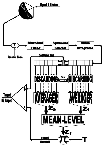
A simplified block diagram of a radar receiver that employs a noncoherent integrator followed by a threshold decision is shown in Fig.1. The input signal to the receiver is composed of the radar
echo signal s(t) and additive zero-mean white Gaussian noisen(t) with varianceσ2.The input noise is assumed to be spatially incoherent and uncorrelated with the signal.The received IF signal is applied to a matched filter which is specifically designed to maximize the output signal-to-noise ratio (SNR).The output of the matched filter is the signalV(t), which can be written as
V(t) =VI(t)cos (ω0t) +VQ(t)sin (ω0t) =r(t)cos (ω0t−θ(t)) (1)
whereω0= 2πf0is the radar operating frequency,r(t) andθ(t) denote
the envelope and phase, respectively, of V(t), and the subscriptsI &
Qrefer to the inphase and quadrature components.
A target is detected when r(t) exceeds the threshold value VT,
where the decision hypotheses are
V(t)
Detection F alse alarm
VT (2)
If the filter output is a complex random variable (RV) that is composed of either noise alone or noise plus target return signal (sine wave of amplitude A), the quadrature components take the forms:
VK(t)
nK(t) +A in the presence of target
nK(t) in the absence of target K=I, Q (3)
The noise quadrature components nI(t) and nQ(t) are uncorrelated
zero-mean low pass Gaussian noise with equal variancesσ2.The joint probability density function (PDF) of them is given by
f(nI, nQ) =
1 2πσ2exp
−n
2 I+n2Q
2σ2
= 1 2πσ2exp
−(rcos(θ)−A)
2
+ (rsin(θ))2 2σ2
(4)
In terms of the joint probability density function of nI(t) and nQ(t),
we can evaluate the joint PDF of the new random variables r(t) and
θ(t) as
f(r, θ) = r
2πσ2exp
−r2+A2
2σ2
exp
rAcos(θ)
σ2
The PDF ofr is obtained by integrating Eq.(5) over θ.Thus,
f(r) = r
σ2exp
−r2+A2
2σ2
I0
rA
σ2
(6)
I0(.) denotes the modified Bessel function of order 0.In the literature,
the above PDF is known as Rice distribution.It is obvious that in the absence of radar target return (A = 0), this distribution tends to Rayleigh PDF.On the other hand, if (rA/σ2) becomes very large,
Eq.(6) tends to Gaussian PDF with mean A and varianceσ2 [9].
2.1. Pulse Integration
When a target is illuminated by the radar beam, it normally reflects numerous pulses.The radar detection probability is enhanced by summing all (or most) of the returned pulses.The process of adding radar echoes from many pulses is known as pulse integration.This process can be performed on the quadrature components prior to or after the envelope detector.The pulse integration in the first case is called coherent or pre-detection while in the second case, it is known as noncoherent or post-detection integration.Coherent integration preserves the phase relationship between the received pulses and consequently, a build up in the signal amplitude is achieved.In post-detection integration, on the other hand, the phase relation is destroyed.In coherent integration of M pulses, it is shown that the signal power after the coherent integrator is unchanged, while the noise power is reduced by the factor 1/M.Therefore, the signal-to-noise ratio (SNR) in the process of coherent integration ofM pulses is improved by M.However, the requirement of reserving the phase of each transmitted pulse as well as maintaining coherency during propagation is very costly and challenging to achieve.For these reasons, most radar systems utilize noncoherent integration owing to its ease of implementation.A block diagram of radar receiver utilizing a square-law detector and a noncoherent integrator is outlined in Fig.1.
Let us now go to calculate the PDF of integrator output.The output of the square-law detector for the th pulse is proportional to the square of its input.Thus, it is convenient to define new variables as
y
r2
2σ2 and Λ1
A2
2σ2 =SN R (7)
given by
fy(y) = exp (−(y+ Λ1))I0
2yΛ1 (8)
Noncoherent integration ofM pulses is implemented as
Y =
M
=1
y (9)
Since the RV’s ri’s are statistically independent, the PDF of Y is [8]
fY(Y /Λ) =
Y
Λ
M−1 2
exp(−(Y + Λ))IM−1(2 √
YΛ) (10)
IM−1(.) represents modified Bessel function of order M −1.The
parameter Λ is the total, M pulse, SNR; Λ = MΛ1 in terms of the
per pulse SNR (Λ1).
2.2. Detection of Fluctuating Targets
So far we assumed a constant target cross section (nonfluctuating target).However, when target scintillation is present, the detection performance decreases due to decreasing the equivalent SNR.
To model the target fading, the total SNR (Λ) is taken to be random with prior PDF of χ2-distribution with κ-degrees of freedom. Thus,
fΛ/Λ=
κ
Λ
κΛκ−1
Γ(κ) exp
−κΛ
Λ
U(Λ) (11)
In the above expression, Λ is the average M-pulse SNR, Γ(.) is the gamma function, and U(.) denotes the unit step function.
In this model, any value ofκ >0 is acceptable.This model takes into account the correlation between noncoherent pulse bursts.In any event, the resulting primary target PDF forχ2 fluctuating target with
κ-degrees of freedom is given by [13]
fY
Y /Λ =
∞
0
fY (Y /Λ)f
Λ/ΛdΛ
=
κ
Λ +κ
κ
YM−1
Γ (M)1F1
κ, M; Λ
Λ +κY
1F1(.) is the confluent hypergeometric function.The characteristic
function (CF) associated with Eq.(12) can be obtained by taking the Laplace transformation of it which results
ΩY(S) =
1
S+ 1
M−κ
1−β
S+ 1−β
κ
, β Λ
κ+ Λ (13)
In the case where κ=M, the above formula tends to the well-known Swerling II (SWII) target fluctuation model.Therefore, when the target fluctuates in accordance with SWII model, its associated CF has a form given by
ΩY(S) =
a
S+a
M
, a 1
1 + Λ1
& Λ1
Λ
M (14)
The Laplace inverse of the previous equation gives the PDF of the SWII target fluctuation model.Thus,
fY(y) =
1 1 +ψ
M
yM−1
Γ(M)exp
− y
1 +ψ
U(y), ψΛ1 (15)
The integrator output is then sampled and the sampling rate is assumed to be such that the successive samples are statistically independent.A set of N samples, called the sample set, is used for the noise level estimation.It is assumed that the sample tested for detection is excluded from this set and thus ensure that the threshold computed by the detector is independent of the tested sample.The sample set is applied to a discarding operation which nullifies any sample that exceeds a predetermined discarding threshold “τ”.The set of surviving samples at the censor’s output is averaged with only the nonzero samples considered.The average value “Z” of the samples is multiplied by a predetermined detection coefficient “T”, which is dependent on the size of the sample set and the required rate of false alarm, and the result of this processing is used as a detection threshold against which the content of the cell under test is compared to decide whether the target under investigation is present or absent.A sample that exceeds this threshold is declared to be detected.
pulse SNR) equals to zero.Thus,
fX(x) =
xM−1
Γ(M)e
−xU(x) (16)
Based on the hypothesis test, the processor detection performance can be evaluated from the well known relation
Pd
∞
0
fZ(z) ∞
ZT
fY(y)dydz (17)
SinceY and Z are statistically independent, lettingν =Y −T Z leads to
Ων(S) = ΩY(S)ΩZ(−T S) (18)
The substitution ofν in the expression of Pd yields
Pd=
∞
0
fν(u)du (19)
The PDF of the random variable ν can be obtained by performing the Laplace inversion of Eq.(18). Thus, performing this inversion and integrating the resulting form with an allowable change in the order of integration gives
Pd=−
res
ΩY(S)
ΩZ(−T S)
S , S
(20)
where the contour of integration lies to the right of all singularities of ΩY(S) in the left half plane and S’s (= 1, 2, . . . ) are the poles of
ΩY(S) and res[.] stands for the residue.
For the Swerling II target fluctuation model, the detection probability can be calculated by substituting Eq.(14) in Eq.(20) which yields [9]
Pd=
T
1 +ψ
M
(−1)M−1 Γ(M)
dM−1
dSM−1 {ΦZ(S)}
S=1+Tψ (21)
where ΦZ(.) stands for the Laplace transformation of the cumulative
distribution function (CDF) of the noise level estimate Z and ψ
It is evident from this derivation that the key step in the processor performance evaluation is the determination of the Laplace transformation of the CDF of its noise power level Z and therefore, we focus our attention, in the following section, on deriving it for the DT-CFAR detector when it is operated in an interference saturated environment from which the homogeneous performance can be easily obtained as a special case by setting the number of interferers equals to zero.
3. PROCESSOR PERFORMANCE ANALYSIS
The corruption of signals with thermal noise represents the basic problem in radar detection.This type of noise originates in both the receiving system and the external environment as a result of natural phenomena.In practical application of radar, the noise that competes with signals may originate in other ways.For military radars, deliberate radiation of jamming signals may introduce additional noise into the receiving system.A CFAR processor is that one which provides a constant false alarm rate against varying conditions in an interference operating environment by adaptively adjusting the detection threshold.The key assumptions in the DT-CFAR detector is that the reference cell variates have the same distribution as that of the cell under test variate in the no target present case.Therefore, when the reference cell variates Xi’s, i = 1, 2, . . ., N, are taken to
be square-law detected and noncoherently integrated Gaussian noise variates, they are statistically independent and identically distributed (IID) random variables of gamma distribution, see Eq.(16). These samples pass through a censor of threshold τ.A sample Q that was not censored is a random variable with a PDF given by
fQ(q)fX(q|x≤τ) =
qM−1
Γ(M)
exp(−q)
1−
M−1
=0
τ
Γ(+1)exp(−τ)
{U(q)−U(q−τ)}
(22)
It is seen, from the above expression that the PDF of Q is the PDF ofXtruncated at the discarding thresholdτ and properly normalized. The probability that a sample survives the censor is
Pt(x≤τ) =
τ
0
fX(x)dx= 1−
M−1
=0
τ
Γ(+ 1)e
On the other hand, the probability that n out of N nonzero samples remain after the discarding operation has the following expression [5]
PS(n;N) =
N n
Ptn(1−Pt)N−n (24)
In order to analyze the performance of the DT detector when the reference window no longer contains radar returns from a homogeneous background, the assumption of statistical independence of the reference cells is retained.The multitarget environment, on the other hand, is the more interesting situation that is frequently encountered in practice in which the window contains nonuniform samples.This may occur in a dense environment where two or more potential targets appear in the reference window.The amplitudes of all the targets present in the reference window are assumed to be fluctuating in accordance with SWII model.Suppose that the sample set contains r returns from spurious targets each of strength 1 +I and n cells contain thermal noise only.The sample mean computed by the detector is
Z 1
n+r
n
k=1
Xtk +
r
=0
Xf
, 0≤r≤R & 1≤n≤N −R
(25)
In the above expression, Xt represents the sample that contains
thermal noise only, while Xf denotes reference cell that contains
interfering target return. n and r denote the number of surviving thermal and interferer samples, respectively.We assume that n ≥ 1, but allow r = 0 which means that all interferer samples are censored. Since the cells of each one of the two random sets are IID, the sample average Z has a CF given by
ΩZ(S) ={ΩXt(S)}n
ΩXf(S)
r
S=nS+r (26)
where
ΩXt(S) =
1
S+ 1
M 1− M−1
=0
τ(S+ 1)
Γ (+ 1) exp (−τ(S+ 1))
1−
M−1
j=0 τj
Γ (j+ 1)exp (−τ)
and
ΩXf(S) =
b
S+b
M 1− M−1
i=0
τi(S+b)i
Γ (i+ 1) exp (−τ(S+b))
1−
M−1
k=0
(bτ)k
Γ(k+ 1) exp (−bτ)
, b 1
1 +I
(28)
LetPn(n) andPr(r) denote the probabilities ofnnoise samples and r
outlying samples surviving the censor, respectively, then
Pn(n;N−R) =
N−R
n
Ptn(1−Pt)N−R−n (29)
wherePtis as previously defined in Eq.(23), and
Pr(r;R) =
R r
Pfr(1−Pf)R−r (30)
and
Pf = 1−
M−1
=0
(bτ)
Γ(+ 1)exp(−bτ) (31)
The parameter b is the same as that defined in Eq.(28). The conditioning onnand r can be removed by averaging Eq.(26). Thus,
ΩZ(S) = N−R
n=1
Pn(n;N−R)
R
r=0
Pr(r;R)
ΩXt
S
n+r
n
ΩXf
S
n+r
r
(32)
The substitution of Eqs.(23), (27), (28) & (31) into Eq.(32) yields
ΩZ(S) = N−R
n=1
N −R
n
M−1
j=0 τj
Γ (j+ 1)e
−τ
N−R−n
R
r=0
R r
M−1
=0
(bτ)
Γ (+ 1)e
−bτ
1−
M−1
i=0
τi(S+ 1)i
Γ(i+ 1) exp (−τ(S+ 1))
(S+ 1)M
n 1−
M−1
k=0
τk(S+b)k
Γ (k+ 1) exp (−τ(S+b))
(S+b)M/bM
r (33)
Once the CF of the noise power level estimate Z is obtained, the processor detection performance can be easily evaluated.Recall that the processor detection performance is completely determined by calculating the Laplace transformation of the CDF of its noise power level estimate.In terms of the CF of Z, we can compute the Laplace transformation of its associated CDF from the well known relation [12]
ΦZ(S) =
ΩZ(S)
S (34)
In order to reduce the processing time taken by the CFAR circuit to decide whether or not the radar target is present, it is recommended that the size of the reference set is to be as small as possible.On the other hand, the processor detection performance is enhanced as the size of the processing set is increased.To solve this contradiction, it is preferable to split the reference set into leading and trailing parts symmetrically about the cell under test.The elements of each subset are processed separately to estimate its noise power level and the two resultant noise power levels are combined through the mean operation to formulate the final noise power level estimate.For this type of CFAR processors, we have
Z1 1 N1 N1 j=1
Xj & Z2
1
N2
N2
=1
X (35)
In the above expression, N1 and N2 represent the sizes of the leading
and trailing subsets, respectively, where N1+N2 =N; the size of the
global reference set.
Suppose that the leading subset hasr1 samples that contain outlying
target returns and hasn1 cells that contain thermal noise only.Then
the estimated noise power level from the leading subset has a form given by
Z1
1
n1+r1
n1
i=1
Xti+
r1
j=0
Xfj
(36)
Similarly, the noise power level estimated from the trailing subset has the same formula as that given in Eq.(36) after replacing n1 & r1
by n2 & r2, respectively.In this case, r2 represents the number of
samples amongst the candidates of the trailing subset that may contain interfering target returns, and n2 denotes those that contain thermal
noise only.Thus,
Z2
1
n2+r2
n
2
k=1
Xtk+
r2
=0
Xf
(37)
The application of the samples of each subset to the discarding threshold will pass those samples of amplitudes less that or equal to it to the averaging processing to construct the associated noise power level to each subset.The final noise power level estimate is obtained by combining these noise level estimates through the mean-level operation.Thus,
Zf mean(Z1, Z2) (38)
By following the same procedure as that of single-window performance evaluation, we can calculate the CF of each one of these noise level estimate.Therefore, Z1 and Z2 have CF’s given by Eq.(33) after replacing its parameters with the corresponding ones of Z1 and Z2. Thus,
ΩZ1(S) =
N1−R1
n1=1
N1−R1
n1
M−1
j=0 τj
Γ (j+ 1)e
−τ
N1−R1−n1
R1
r1=0
R1 r1
M−1
=0
(bτ) Γ (+ 1)e
−bτ
1−
M−1
i=0
τi(S+ 1)i
Γ(i+ 1) exp (−τ(S+ 1))
(S+ 1)M
n1 1−
M−1
k=0
τk(S+b)k
Γ(k+ 1) exp (−τ(S+b))
(S+b)M/bM
r1 (39) and
ΩZ2(S) =
N2−R2
n2=1
N2−R2
n2
M−1
j=0 τj
Γ (j+ 1)e
−τ
N2−R2−n2
R2
r2=0
R2
r2
M−1
=0
(bτ)
Γ (+ 1)e
−bτ
R2−r2
1−
M−1
i=0
τi(S+ 1)i
Γ(i+ 1) exp (−τ(S+ 1))
(S+ 1)M
n2 1−
M−1
k=0
τk(S+b)k
Γ(k+ 1) exp (−τ(S+b))
(S+b)M/bM
r2 (40)
Since the noise level estimatesZ1 andZ2 are statistically independent,
the final noise power level estimate Zf has a CF that is given by the
product of their characteristic functions.Hence,
ΩZf(S) = ΩZ1(S)ΩZ2(S) (41)
detection which becomes
Pd=
T
1 +ψ
M
(−1)M−1 Γ(M)
dM−1
dSM−1
ΦZf(S) S= T
1+ψ
(42)
where the Laplace transformation of the CDF of the final noise level estimate Zf can be easily obtained by substituting Eq.(41) into
Eq.(34).
Once the Laplace transformation of CDF of the final noise level estimate is calculated, the processor performance evaluation becomes an easy task as Eq.(42) demonstrates.
4. PERFORMANCE EVALUATION RESULTS
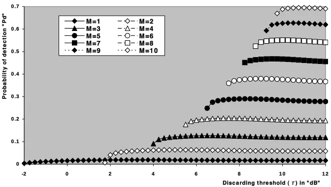
In this section, we are going to give some numerical results to demonstrate the validity of our analysis as well as to obtain an idea about the behavior of DT-CFAR processor under noncoherent integration of M pulses when the operating environment contains an intense number of outlying targets along with the target under investigation.These results include the processor detection and false alarm performances.The set of figures presented here provides some insight into the influence of the various variables on the detector’s performance, and therefore assists in the design of proper procedures for determination of the detector parameters.Owing to the importance of the SWII target fluctuation model in practical applications, we focus our numerical results to this model for the primary and the secondary extraneous targets.All our results are calculated for a sample set of size 24 and a design false alarm rate of 10−6.Fig.2 displays the detection probability as a function of the discarding thresholdτ when the radar receiver noncoherently integrates M pulses and operates in an environment which is free of spurious targets.The strength of the primary target return (SNR) is assumed to be 5 dB.It is obvious from the results of this figure that asM increases, the critical value of the discarding threshold “τc” increases.This critical value is defined as
the number of noncoherently integrated pulses increases.For example, the detection probability equals 0.0164 for single sweep case (M = 1) while it attains a value of 0.688 when 10 consecutive sweeps (M = 10) are integrated to represent the input of the decision circuit, given that the discarding threshold is held constant at 10 dB.This example demonstrates to what extent the processor detection performance will be enhanced with noncoherent integration ofM pulses.
0 0 .1 0 .2 0 .3 0 .4 0 .5 0 .6 0 .7
-2 0 2 4 6 8 1 0
Disc a rding t hre shold (τ) in "dB"
P
ro
b
a
b
il
it
y
o
f
d
e
te
c
ti
o
n
"
P
d
"
1 2
M =1 M =2
M =3 M =4
M =5 M =6
M =7 M =8
M =9 M =1 0
Figure 2. M-sweeps ideal detection performance, as a function of the discarding threshold, of the double-threshold adaptive processor when
N = 24, SNR = 5 dB, and Pf a = 1.0E-6.
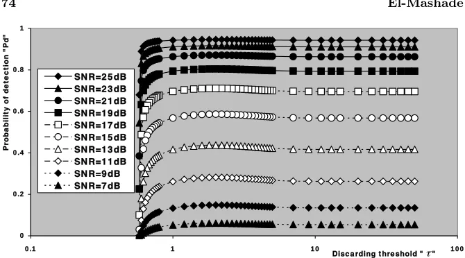
To show the effect of changing the signal strength on the detection probability, let us go to plot, in Fig.3, the same characteristics for several values of SNR after fixingM(at single sweep case) and allowing the reference channels to be contaminated with 5 (R =R1+R2 = 5)
interfering target returns of relative strength (INR/SNR) of −5 dB. It is shown that the critical value of τc is 0.58 dB, in the case of
single sweep (M = 1), below which there is no detection (Pd =
0), as it is previously defined.As the SNR increases, there is an improvement in the multitarget detection performance of the processor under consideration.For a specified SNR, the detection probability starts to increase at τc till it attains its maximum value after which
0 0 .2 0 .4 0 .6 0 .8 1
0 .1 1 1 0 1 0 0
Disc a rding t hre shold "τ"
P
ro
b
a
b
il
it
y
o
f
d
e
te
c
ti
o
n
"
P
d
"
SN R=2 5 dB SN R=2 3 dB SN R=2 1 dB SN R=1 9 dB SN R=1 7 dB SN R=1 5 dB SN R=1 3 dB SN R=1 1 dB SN R=9 dB SN R=7 dB
Figure 3. Single sweep multitarget detection performance of the double-threshold CFAR scheme, as a function of the discarding threshold, whenN = 24,R= 5, INR/SNR =−5 dB, and Pf a = 1.
0E-6.
higher values of this important parameter.
1 .0 E-0 5 1 .0 E-0 4 1 .0 E-0 3 1 .0 E-0 2 1 .0 E-0 1 1 .0 E+0 0
-1 0 -6 -2 2 6 1 0 1 4 1 8 2 2 2 6 3
I nt e rfe re nc e -t o-noise ra t io (I N R) "dB"
P
ro
b
a
b
il
it
y
o
f
d
e
te
c
ti
o
n
"
P
d
"
0 α = 0, τ = 2.5
α = 5, τ = 2.5 α = 10, τ = 2.5
α = 0, τ = 5.0 α = 5, τ = 5.0 α = 10, τ = 5.0
α = 0, τ = 7.5 α = 5, τ = 7.5 α = 10, τ = 7.5
α = 0, τ = 10 α = 5, τ = 10 α = 10, τ = 10
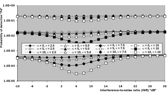
Figure 4. M-sweeps detection performance, as a function of the interference strength, of the double-threshold CFAR scheme when
N = 24, M = 1, R= 5, andPf a= 1.0E-6.
role in constructing the detection threshold which becomes augmented and consequently the detection probability is decreased.For higher values of interference level, on the other hand, the discarding threshold eliminates the outlying target returns from the contents of the reference set leaving those of thermal noise only to be used in estimating the unknown noise power level.In this case, the candidates of the reference set become to be homogeneous resulting in decreasing the detection threshold and this in turn improves the probability of detection.In this discussion, it is assumed that the discarding threshold is held unchanged (τ = constant).For lower values of τ, the previous phenomena is not clearly demonstrated and the detection probability seems to be constant irrespective to the level of interference.As the discarding threshold increases, the explained phenomena is explicitly illustrated.On the other hand, if the strength of the primary target return becomes higher (α = 10 dB), the presence of outlying target returns amongst the candidates of the reference set has little effect on the processor detection performance.
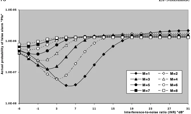
In the second category of our numerical results, we are concerned with the processor false alarm rate performance as a function of the interference strength excited by outlying targets for several values of discarding threshold when the processing data are collected from M
1 .0 E-0 8 1 .0 E-0 7 1 .0 E-0 6 1 .0 E-0 5
-5 -1 3 7 1 1 1 5 1 9 2 3 2 7 3 1
I nt e rfe re nc e -t o-noise ra t io (I N R) "dB"
A
c
tu
a
l
p
ro
b
a
b
il
it
y
o
f
fa
ls
e
a
la
rm
"
P
fa
"
M =1 M =2
M =3 M =4
M =5 M =6
M =7 M =8
Figure 5. M-sweeps actual probability of false alarm, as a function of the interference strength, of the double-threshold CFAR detector when
N = 24, τ = 10 dB,R= 5, and designPf a= 1.0E-6.
1 .0 E-1 0 1 .0 E-0 9 1 .0 E-0 8 1 .0 E-0 7 1 .0 E-0 6 1 .0 E-0 5
-5 -1 3 7 1 1 1 5 1 9 2 3 2 7 3 1
I nt e rfe re nc e -t o-noise ra t io (I N R) "dB"
A
c
tu
a
l
p
ro
b
a
b
il
it
y
o
f
fa
ls
e
a
la
rm
"
P
fa
"
M =1 M =2
M =3 M =4
M =5 M =6
M =7 M =8
Figure 6. M-sweeps actual probability of false alarm, as a function of the interference strength, of the double-threshold CFAR detector when
1 .0 E-1 5 1 .0 E-1 3 1 .0 E-1 1 1 .0 E-0 9 1 .0 E-0 7 1 .0 E-0 5
-5 -1 3 7 1 1 1 5 1 9 2 3 2 7 3 1
I nt e rfe re nc e -t o-noise ra t io (I N R) "dB"
A
c
tu
a
l
fa
ls
e
a
la
rm
p
ro
b
a
b
il
it
y
"
P
fa
"
M =1 M =2 M =3 M =4 M =5 M =6 M =7 M =8
Figure 7. M-sweeps actual probability of false alarm, as a function of the interference strength, of the double-threshold CFAR detector when
N = 24, τ = 20 dB,R= 5, and designPf a= 1.0E-6.
reference channels are assumed to be contaminated by 5 interfering target returns.The designed false alarm rate is, as previously stated, taken to be 10−6.Generally, the presence of spurious target returns amongst the candidates of the reference channels raises the decision threshold and consequently decreases the false alarm rate.Since the decision threshold is constructed on the basis that the elements of the reference set are homogeneous; i.e., free from any other object returns except the clear background, any reason for making these samples nonhomogeneity degrades the processor performance.When the strength of outlying targets is modest, their corresponding cells succeed to escape from the discarding threshold and hence they play an important role in establishing the decision threshold.In other words, if the interference level is of low value that makes the extraneous target returns to be smaller than the excising threshold, the setting of the decision threshold must take into account these returns.As a result of them, the decision threshold becomes of higher value than that proposed in the case where the contents of the reference set are homogeneous.Increasing the decision threshold means decreasing the probability of detection either the target is present (Pd) or the
target is absent (Pf a).As the interference level (INR) increases, the
that making the strength of interferers to be comparable with the discarding threshold, the reference channels start to be purged from their returns and step-by-step the content of the reference set tends to be again homogeneous.This behavior will lead to improve the false alarm probability towards its design value.In the above explanation, it is assumed that the number of noncoherently integrated pulses is held constant.On the other hand, if the number of integrated pulses increases, the effective value of the interfering target returns increases and consequently the probability of excising them also increases leaving only the clear background samples to be used in noise level estimation and hence the probability of false alarm will be improved.This means that, as M increases, the interference level, at which the false alarm rate starts to be explicitly degraded, decreases and that level at which Pf a starts to be improved, after it attains its worst value,
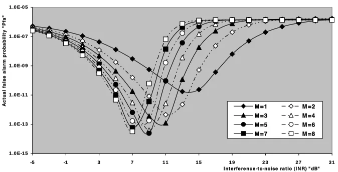
also decreases, as Fig.5 illustrates this behavior. In other words, the interference level, at which the false alarm attains its worst rate, as well as the value of this worst rate will be lowered as the number of noncoherently integrated pulses increases, given that the excision threshold rests unchanged.Fig.6 shows the same characteristics while the censoring threshold is changed from 10 dB to 15 dB under the same operating conditions as in Fig.5. The displayed results illustrate that increasing the discarding threshold degrades the processor false alarm rate performance drastically along with making the worst false alarm rate more severe.In addition, the interference level at which the false alarm rate attains its worst value is shifted towards higher values of INR.This result is predicted because increasing τ means increasing the effective value of interfering target return at which it is discarded. To verify this prediction, we repeat the same characteristics in Fig.7 after setting τ to 20 dB.Similar comments can be extracted from the behavior of the curves of the underlined figure.
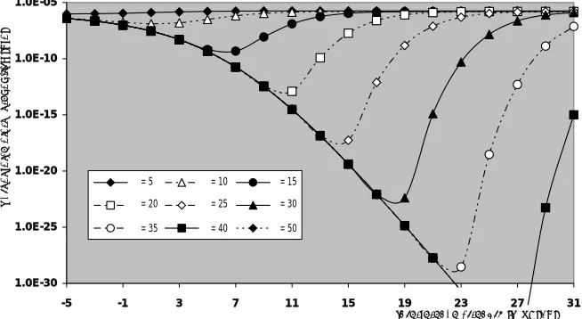
In order to confirm our anticipation about the false alarm rate performance of the processor under investigation, we focus our attention in the next group of displayed results, Figs.8–9, on the same behavior, as in the previous set of curves, when the parameters M
and τ vary simultaneously.Four values are chosen for each one of the underlined parameters: M = 1, 2, 4, 5, and τ = 10, 20, 30, 50 dB.The single sweep results are considered here as a reference with which the noncoherent integration of M-pulses is compared.Firstly, let us take the parameter M to be fixed and make the parameter τ
1 .0 E-3 0 1 .0 E-2 5 1 .0 E-2 0 1 .0 E-1 5 1 .0 E-1 0 1 .0 E-0 5
-5 -1 3 7 1 1 1 5 1 9 2 3 2 7 3 1
I nt e rfe re nc e st re ngt h (I N R) "dB"
A
c
tu
a
l
fa
ls
e
a
la
rm
p
ro
b
a
b
il
it
y
"
P
fa
"
M = 1, τ = 10 M = 2, τ = 10 M = 4, τ = 10 M = 5, τ = 10 M = 1, τ = 20 M = 2, τ = 20 M = 4, τ = 20 M = 5, τ = 20 M = 1, τ = 30 M = 2, τ = 30 M = 4, τ = 30 M = 5, τ = 30 M = 1, τ = 50 M = 2, τ = 50 M = 4, τ = 50 M = 5, τ = 50
Figure 8. M-sweeps actual false alarm probability of the double-threshold CFAR scheme as a function of the interference strength, when N = 24, R= 5, and designPf a= 1.0E-6.
1 .0 E-3 0 1 .0 E-2 5 1 .0 E-2 0 1 .0 E-1 5 1 .0 E-1 0 1 .0 E-0 5
-5 -1 3 7 1 1 1 5 1 9 2 3 2 7 3 1
I nt e rfe re nc e st re ngt h (I N R) "dB"
A
c
tu
a
l
fa
ls
e
a
la
rm
p
ro
b
a
b
il
it
y
"
P
fa
"
τ = 5 τ = 10 τ = 15
τ = 20 τ = 25 τ = 30
τ = 35 τ = 40 τ = 50
Figure 9. M-sweeps actual false alarm probability of the double-threshold CFAR scheme as a function of the interference strength, when N = 24, M = 3,R= 5, and design Pf a = 1.0E-6.
return to its designed value.On the other hand, increasingM makes the rate of decreasing of false alarm rate to be rapidly increased as well as decreases the interference level, at which the probability of false alarm begins to be augmented on focusing to attain its steady state value.The numerical results presented in this scene give a good idea about the reaction of the DT-CFAR detector against the number of noncoherently integrated pulses and the variation of the excision threshold when the operating environment contains an intense number of outlying targets along with the target under test.It is of importance to note that asτ becomes very high (τ → ∞), the DT scheme behaves like the well-known cell-averaging (CA) procedure in its false alarm and detection performances.Before discussing the ineffectiveness zone of the processor under consideration, attention should be drawn to the following conclusion: when interferers are discarded from the sample set, the noise power estimation is based on a smaller number of samples and, if the detection threshold is taken as its initial value, computed in the absence of extraneous targets (R = 0), the false alarm rate increases.This behavior is clearly shown in Fig.9 which illustrates the double-threshold false alarm rate performance as a function of the strength of interfering targets (INR) for several values of τ when three consecutive sweeps are noncoherently integrated (M = 3) to prepare the data from which the detection threshold is established. The number of reference cells that are contaminated by interfering target returns is 5.For this family of curves, the notation (τ = 5) on a specified curve indicates that it is plotted forτ = 5 dB.It is observed that for low values of the censoring threshold τ, the false alarm probability remains approximately constant with small deviations, from its designed value, for weakly extraneous targets and these deviations are rapidly decreased as either the interfering strength or the number of noncoherently integrated pulses increases.Whenτ tends to infinity, Pf a decreases rapidly with INR, since all the interferers
are survived and their presence amongst the elements of reference set raises the detection threshold which consequently decreases the false alarm rate intolerably.In other words, for smaller values of the discarding threshold, the false alarm rate remains approximately constant irrespective of the interference strength.In that case, it is obvious that all the interferer returns are eliminated from the reference window and the construction of the detection threshold is actually a direct translation of the homogeneous background and consequently the false alarm rate is independent of the interference level.As τ
alarm.This process is continued till the interference level becomes strong.In that case, the interferer returns are completely discarded and they have no influence on the setting of the detection threshold. Because of this, the false alarm rate tends to be constant.Based on this behavior, we define what we will call ineffectiveness zone of the double-threshold detector.This zone is defined as the range below the excision threshold in which the spurious target returns succeed to escape from the discarding threshold and therefore they have a direct effect on the setting of the detection threshold.Asτ increases, the location of this zone is shifted towards the higher interference level.In the limit, asτ
0 0 .2 0 .4 0 .6 0 .8 1
-5 -1 3 7 1 1 1 5 1 9 2 3 2 7 3 1
Prim a ry t a rge t signa l-t o-noise ra t io (SN R) "dB"
P
ro
b
a
b
il
it
y
o
f
d
e
te
c
ti
o
n
"
P
d
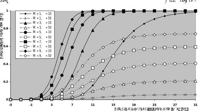
" M = 1, τ = 10 M = 1, τ = 50 M = 3, τ = 10 M = 3, τ = 50 M = 5, τ = 10 M = 5, τ = 50 M = 7, τ = 10 M = 7, τ = 50 M = 9, τ = 10 M = 9, τ = 50
Figure 10. Multipulse detection performance of double-threshold adaptive processor operating in multitarget environment whenN = 24,
R= 5,α= 1 and Pf a= 1.0E-6.
the other hand, the detection probability forτ = 10 dB is higher than that for τ = 50 dB, given that M is held unchanged.This behavior is predicted since the probability of eliminating the interfering target returns in the case of τ = 10 dB is higher than that in the case of
0 0 .2 0 .4 0 .6 0 .8 1
-5 -1 3 7 1 1 1 5 1 9 2 3 2 7 3 1
Prim a ry t a rge t signa l-t o-noise ra t io (SN R) "dB"
P
ro
b
a
b
il
it
y
o
f
d
e
te
c
ti
o
n
"
P
d
"
M = 1, τ = 5 M = 2, τ = 5 M = 1, τ = 10 M = 2, τ = 10 M = 1, τ = 15 M = 2, τ = 15 M = 1, τ = 20 M = 2, τ = 20 M = 1, τ = 25 M = 2, τ = 25
Figure 11. M-sweeps multitarget detection performance of the double-threshold adaptive processor when N = 24, R = 5, α = 1 and Pf a = 1.0E-6.
0 0 .2 0 .4 0 .6 0 .8 1
0 3 6 9 1 2 1 5
N um be r of spurious t a rge t s "R"
P
ro
b
a
b
il
it
y
o
f
d
e
te
c
ti
o
n
"
P
d
"
M =1 M =2 M =3
M =4 M =5 M =6
Figure 12. M-sweeps multitarget detection performance of the double-threshold CFAR scheme as a function of the outlying target returns when N = 24, τ = 10 dB, SNR = 10 dB, α = 1, and
0 0 .2 0 .4 0 .6 0 .8 1
0 3 6 9 1 2
N um be r of spurious t a rge t s "R"
P
ro
b
a
b
il
it
y
o
f
d
e
te
c
ti
o
n
"
P
d
"
1 5
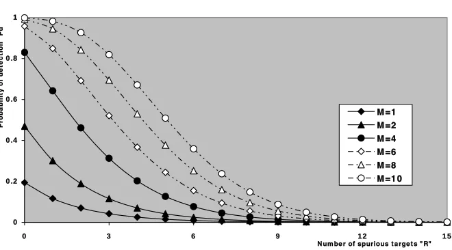
M =1 M =2 M =4 M =6 M =8 M =1 0
Figure 13. M-sweeps multitarget detection performance of the double-threshold CFAR scheme as a function of the outlying target returns when N = 24, τ = 50 dB, SN R = 10 dB, α = 1, and
Pf a = 1.0E30-6.
as the number of outlying target returns increases because of the contribution of them on establishing the detection threshold where there is no chance to excise these returns from the estimation set.This situation corresponds to the well-known CA processor.Generally, asM
increases, the processor performance improves and the required SNR to achieve a specified value of detection probability decreases, eitherτ
is chosen low or high.
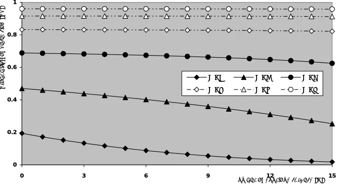
The last subgroup of detection performance is devoted to the presentation of the improvement of detection probability with the number of noncoherently integrated pulses.It contains Figs.14–15. In these figures, the probability of detection is plotted, against the number of integrated pulses M, in the absence (R = 0) as well as in the presence of five outlying target returns amongst the cells of the reference set for various values of the strength of primary target return and for α = INR/SNR = 1.For small numbers of integrated pulses, the homogeneous processor performance exceeds its multitarget detection performance.As M increases, the gap between the two performances is gradually reduced till they become coincide on one another.This behavior is noted for each preassigned value of SNR. Additionally, the value ofM, at which the homogeneous performance coincides with the multiple-target one, decreases as the signal return becomes strengthened.Moreover, increasing SNR improves both the homogeneous and the multitarget processor performances.
Now, let us repeat the same results of Fig.14 after changing the excision threshold from 10 dB to 30 dB and holding the operating conditions unchanged.The obtained results are displayed in Fig.15. In this case, the gap between the homogeneous and the multitarget performances increases and there is no chance for the coincidence of the two performances although M attains large values (M = 10).As noted earlier, increasingτ means increasing the probability of escaping the interfering target returns from the discarding threshold and consequently raising the detection threshold which leads to lowering the detection probability.The curves of this figure vary in the same manner as those of the previous figure.The chance for the absence and the presence of extraneous target return’s performances to be coincide increases as either M, SNR or both of them increases.For our numerical results to be comparable, the single-sweep behaviors are incorporated in constructing the underlined figures.
1 .0 E-0 6 1 .0 E-0 5 1 .0 E-0 4 1 .0 E-0 3 1 .0 E-0 2 1 .0 E-0 1 1 .0 E+0 0
0 1 2 3 4 5 6 7 8 9
N um be r of nonc ohe re nt ly int e gra t e d pulse s "M "
P
ro
b
a
b
il
it
y
o
f
d
e
te
c
ti
o
n
"
P
d
"
1 0
SN R=-5 dB, R=0 SN R=-5 dB, R=5 SN R=0 dB, R=0 SN R=0 dB, R=5 SN R=0 5 dB, R=0 SN R=0 5 dB, R=5 SN R=1 0 dB, R=0 SN R=1 0 dB, R=5
Figure 14. M-sweeps detection performance of the double-threshold CFAR scheme in the absence as well as in the presence of extraneous targets whenN = 24,α= 1, τ = 10 dB, and Pf a= 1.0E-6.
1 .0 E-0 6 1 .0 E-0 5 1 .0 E-0 4 1 .0 E-0 3 1 .0 E-0 2 1 .0 E-0 1 1 .0 E+0 0
0 1 2 3 4 5 6 7 8 9
N um be r of nonc ohe re nt ly int e gra t e d pulse s "M "
P
ro
b
a
b
il
it
y
o
f
d
e
te
c
ti
o
n
"
P
d
"
1 0 SNR=-5dB, R=0 SNR=-5dB, R=5 SNR=0 dB, R=0 SNR=0 dB, R=5 SNR=5 dB, R=0 SNR=5 dB, R=5 SNR=10dB, R=0 SNR=10dB, R=5
Figure 15. M-sweeps detection performance of the double-threshold CFAR scheme in the absence as well as in the presence of extraneous targets whenN = 24,α= 1, τ = 30 dB, and Pf a= 1.0E-6.
4 8 1 2 1 6 2 0 2 4 2 8 3 2 3 6 4 0
0 0 .1 0 .2 0 .3 0 .4 0 .5 0 .6 0 .7 0 .8 0 .9 1
Pre de fine d de t e c t ion proba bilit y "Pd"
R e q u ir e d s ig n a l-to -n o is e r a ti o ( d B )
τ = 2.5
τ = 20
τ = 7.5
τ = 25
τ = 10 τ = 30
τ = 15
Figure 16. Monopulse required signal strength to achieve an operating point of (Pd, 1.0E-6) of the DT-CFAR scheme in the presence
of 5 outlying targets of the same strength as the primary target (α = 1) when N = 24.
0 5 1 0 1 5 2 0 2 5 3 0
0 0 . 1 0 . 2 0 . 3 0 . 4 0 . 5 0 . 6 0 . 7 0 . 8 0 . 9 1
P r e d e f i n e d d e t e c t i o n p r o b a b i l i t y " P d "
R e q u ir e d s ig n a l-t o -n o is e r a t io ( d B )
τ = 5.0
τ = 20
τ = 7.5
τ = 25
τ = 10 τ = 30
τ = 15
Figure 17. M-sweeps required signal strength to achieve an operating point of (Pd, 1.0E-6) of the double-threshold scheme in the presence of
5 outlying targets whenN = 24, α= 1, andM = 3.
τ in dB.For lower values ofτ, the required SNR to achieve a specified detection level is small and increases gradually as Pd increases.Each
curve of Fig.16 can be divided into three regions from the rate of increasing point of view.In the first region (Pd<10%), the increasing
rate is relatively high.In the medium region (10%≤Pd ≤90%), the
increasing rate is relatively low, while in the third region (Pd>90%),
the rate of increasing is higher than those in the previous two regions. Additionally, as τ increases, the slope of the first region increases while the slope of other two regions rest approximately unchanged.To illustrate the effect of noncoherent integration on reducing the required SNR, the results of this figure are repeated under the same operating conditions taking into account that the radar receiver integrates three consecutive pulses before processing data to estimate the unknown noise power level.The obtained numerical values are displayed in Fig.17, which shows the same variation for the required SNR with the predefined detection level.For the same detection level, the required SNR for M = 3 is much smaller than that required for monopulse operation.For example, if Pd=0.5, the required SNR’s are 15 dB
and 8.64 dB for M = 1 and 3, respectively, given that the excision threshold is held constant at 10 dB in the two cases.This numerical example demonstrates the importance of noncoherent integration in enhancing the detection performance of the CFAR processor.As the discarding threshold becomes large, the multiple-target processor performance becomes considerably degraded.This behavior is intuitive since increasing τ increases the number of reference cells used in noise power level estimation, together with an inevitable violation of the inherent assumption that the estimation cells are identically distributed and properly represent the noise in the detection cell.In addition, the likelihood that an interfering target or a spiky clutter return has entered the reference window is obviously larger for larger
τ.On the other hand, once the estimator has been captured by the extraneous target, the primary target is less suppressed by increasing the number of noncoherently integrated pulses.
5 1 0 1 5 2 0 2 5 3 0 3 5 4 0 4 5
5 1 0 1 5 2 0 2 5 3 0 3 5 4 0 4
D i sc a r d i n g t h r e sh o l d (τ) " d B "
R
e
q
u
ir
e
d
S
N
R
"
d
B
"
5
M = 1 M = 2
M = 3 M = 4
M = 5 M = 6
Figure 18. M-sweeps multitarget required SNR to achieve an operating point of (9.0E-1, 1.0E-6) of the double-threshold adaptive detector whenN = 24,R= 5, and α= 1.
0 4 8 1 2 1 6 2 0 2 4 2 8 3 2 3 6 4 0
0 1 2 3 4 5 6 7 8 9 1
N um be r of nonc ohe re nt ly int e gra t e d pulse s "M "
R
e
q
u
ir
e
d
s
ig
n
a
l-to
-n
o
is
e
r
a
ti
o
"
d
B
"
0
τ = 10
τ = 20
τ = 30
τ = 40
τ = 15
τ = 25
τ = 35
τ = 50
Figure 19. M-sweeps multitarget required SNR to achieve an operating point of (9.0E-1, 1.0E-6) of the DT-CFAR processor when
censoring threshold.This behavior is common for all values ofM with the exception that the required SNR decreases as M increases and the rate of decreasing decreases with increasing M.The slope of the curves in the linear part of these characteristics is approximately the same and the critical value of τ increases asM increases, as we have previously explained.In Fig.19, the required SNR is plotted against
M and parametric in τ under the same operating conditions.The displayed results of this figure anticipate the previous conclusions and similar comments can be extracted from the displayed results of this figure.
5. SUMMARY AND DISCUSSION
An interference saturated environment is frequently encountered in radar application.This situation is nominated as multitarget in the radar terminology.In order to improve the detection performance of an adaptive processor in such type of operating environments, it is of importance to purge the interfering target returns from the estimation cells prior the processing of estimation in order to avoid their contribution on the construction of the detection threshold.However, the elimination of the contaminated samples from the candidates of the reference set reduces the size of the estimation cells.To compensate for this reduction, the technique of noncoherent integration of M consecutive pulses is a promising processing to enhance the detection behavior of the CFAR processor.In this manuscript, we analyze the detection performance the double-threshold (DT) CFAR scheme designed to operate in an interference saturated environment, in which the well-known CA processor fails to detect the target under consideration owing to the inevitable influence of the spurious samples on the establishing of the detection threshold, when the radar receiver contains a video integrator amongst its basic elements.Closed form expressions are derived for the false alarm and detection probabilities in the case where there is an intense number of outlying target returns amongst the estimation cells.The primary and the secondary spurious targets are assumed to be fluctuating in accordance with χ2