COMPUTATION OF PHYSICAL OPTICS INTEGRAL BY LEVIN’S INTEGRATION ALGORITHM
A. C. Durgun and M. Kuzuoˇglu
Electrical and Electronics Engineering Department Middle East Technical University
Turkey
Abstract—In this paper, a novel algorithm for computing Physical Optics (PO) integrals is introduced. In this method, the integration problem is converted to an inverse problem by Levin’s integration algorithm. Furthermore, the singularities, that are possible to occur in the applications of Levin’s method, are handled by employing trapezoidal rule together with Levin’s method. Finally, the computational accuracy of this new method is checked for some radar cross section (RCS) estimation problems performed on flat, singly-curved and doubly-singly-curved PEC plates which are modeled by 8-noded isoparametric quadrilaterals. The results are compared with those obtained by analytical and brute force integration.
1. INTRODUCTION
Since the start of widespread application of radars, many numerical techniques have been developed for electromagnetic scattering problems. Even though there are more advanced methods in the literature, Physical Optics (PO) is still a powerful tool for radar cross-section (RCS) estimation problems because of its straightforward implementation and accuracy at high frequencies. Starting from the Stratton-Chu equations, one may obtain the expression for the PO scattered magnetic field in frequency domain, in terms of the wave number (k), the polarization vector of the incident magnetic field ( ¯H0), the normal vector of the scatterer surface (ˆn), the position vector of the scatterer surface (¯r) and the distance of the observer to the origin of the reference frame (R0), as given in (1). In this equation, the integration is done over the illuminated surface of the scatterer (S) and
the unit vectors in the scattering and incidence directions are denoted by ˆks and ˆki, respectively.
¯
Hs= −jke
−jkR0
4πR0
S
2ˆn×H0¯ ׈ksejk(
ˆ
ks−kˆi)·¯r
dS (1)
Due to the complex exponential term, the integrand of the PO integral given in (1) is a very oscillatory function, especially at high frequencies. Therefore, it is very expensive to compute these kinds of integrals by simple numerical integration techniques. Some special techniques are needed in order to compute these integrals accurately and effectively. In fact, there are many techniques on this subject in the literature.
One of these methods is suggested by Ludwig, in which the integration domain is divided into small planar sub domains and on each of them the amplitude and phase components of the integrand are approximated by first degree polynomials [1–3]. The most significant disadvantage of this method is that, since planar sub-domains are used to model the integration domain, too many facets are needed for the accuracy of the computation, particularly around the regions where the curvature is high when compared with the wavelength. Consequently, this situation leads to a very long integration time. To overcome this deficiency of the linear phase approximation, more advanced methods have been introduced which employ curved patches approximated by second degree polynomials for target modeling [4].
Apart from the aforementioned techniques, another frequently used approach to compute the integrals of functions with rapid oscillations is Filon’s method as given in [5]. However, Filon’s method is only applicable to the integrals in which the phase variation of the integrand is linear. In cases of nonlinear phase variations, a modified version of this method may be employed [6].
Another application of Filon’s method available in the literature is used in monostatic RCS computation by PO approximation. In this method, Fubini’s and Stokes theorems are employed to convert the surface integrals into a summation of oscillatory line integrals which are computed by Filon’s method [7]. In addition to this approach, some other methods have been employed to reduce the surface integral to a line integral [8, 9].
integration technique is discussed. The organization of the paper is as follows: In the second part, the theory of Levin’s method is explained. The third part is dedicated to the application of Levin’s method to PO integrals together with the techniques handling the possible singularities that may occur during the computation. In the fourth part, some numerical results, including the RCS computations of flat, singly curved and doubly curved plates, are given and compared with analytical and brute force integration results. Finally, in the last part some concluding remarks are done together with a discussion of advantages and disadvantages of this method.
2. LEVIN’S INTEGRATION METHOD
2.1. One Dimensional Case
One dimensional oscillatory integrals may be expressed in the following form:
I =
b
a
f(x)ejq(x)dx (2) In this integral, iff is a smooth and nonoscillatory function and if the condition |q(x)| (b−a)−1 is satisfied, then this integral can easily be computed using only a small number of values off andq in [a, b].
In his paper, Levin proposed that iff is of the form
f(x) =jq(x)p(x) +p(x)≡L(1)p(x) (3) then the integral can be evaluated as
I =
b
a
d dx
p(x)ejq(x)
dx=p(b)ejq(b)−p(a)ejq(a) (4)
where the general solution for pis given as
p(x) =e−jq(x)
⎛ ⎝
x
a
f(t)ejq(t)dt+c
⎞
⎠ (5)
The general solution for p(x) is also as oscillatory as the integral in the Equation (5). However, iff and q are slowly varying, then there exists a slowly varying particular solutionp0 of (3). Then the result of the integral in (2) can be expressed as
2.2. Two Dimensional Case
The two dimensional approach of Levin’s method is very similar to one dimensional problem. In this case, a two dimensional oscillatory integral is to be solved which is in the form:
I =
b
a d
c
f(ξ, η)ejq(ξ,η)dξdη (7)
In order to apply the Levin’s method to this kind of integrals, f should be smooth and nonoscillatory as in the one dimensional case. However, the conditions that should be satisfied byq are expanded to two dimensional space.
∂q∂ξ=|qξ| (b−a)−1
∂η∂q=|qη| (d−c)−1
(8)
In addition to this, a new operator should be defined instead of the operator given in Equation (3). The new operator is:
L(2)(p) =pξη+jqξpη +jqηpξ+ (jqξη−qξqη)p=f (9)
Then, by using the Equation (10)
∂2 ∂ξ∂η(pe
jq) = (
pξη +jqξpη+jqηpξ+ (jqξη −qξqη)p)ejq (10)
one can show that the solution of the integral in (7) is equal to
⇒I =p(b, d)ejq(b,d)−p(a, d)ejq(a,d)−p(b, c)ejq(b,c)+p(a, c)ejq(a,c) (11) After this point, ann-point collocation approximation can be made to the functionp(x) in terms of some linearly independent basis functions uk,
pn(x) = n
k=1
akuk(x) (12)
where the coefficients ak are determined by the n collocation
conditions. Now, the problem reduces to finding the coefficients ak.
If we substitute Equation (7) into Equation (3), we get
pn= n
k=1
akuk ⇒L(2)
n
k=1 akuk
(ξj, ηj) =f(ξj, ηj)
{uk(ξ, η)}nk=1=
ξiηj0≤i, j≤√n−1
Equation (13) can easily be converted to the form of Ax = b, where A, b and xare defined as follows:
⎡ ⎢ ⎣
L(2)u1(¯x1) L(2)u2(¯x1) . . . L(2)un(¯x1)
..
. ... ... ... ...
L(2)u1(¯xn) L(2)u2(¯xn) . . . L(2)un(¯xn) ⎤ ⎥ ⎦
⎡ ⎣ a1...
an ⎤
⎦=
⎡ ⎣f
(¯x1) .. . f(¯xn)
⎤ ⎦
(14) where each ¯xi is a collocation point. In this study, only 9 collocation
points are used which are selected to be the 4 corner points (a, c),(a, d),(b, c),(b, d), 4 mid points (a,c+2d),(b,c+2d),(a+2b, c),(a+2b, d) and 1 central point (a+2b,c+2d).
Therefore, it is enough to solve this system of linear equations to find the result of the integral given in Equation (7). Note that in Equation (13), two dimensional monomials are used as basis functions. The selection of basis functions and their number may affect the computational cost significantly. Throughout this study, the monomials up to 2nd order are used as basis functions, for both one and two dimensional cases, and it is observed that, this selection gives very accurate results with sufficiently low computational cost. In view of the fact that it is out of the scope of this paper, the effects of using other kinds of basis functions to the results may also be investigated as a future work.
3. COMPUTATION OF THE PO INTEGRAL
The procedure explained in the previous section is only applicable to integrals defined on rectangular domains in two dimensional spaces. However, in radar cross section problems, the integration domain is generally an arbitrary three dimensional surface and the integrals are in the form of Equation (15). Therefore, a special treatment is needed to use Levin’s method to RCS problems.
I =
ϕ
f(x, y, z)ejq(x,y,z)dϕ (15)
Let ϕ= (x, y, z) be an arbitrary surface in 3. It is possible to map any surface ϕ to a rectangular domain [−1,1]×[−1,1] in (ξ, η) local coordinates [11].
y and z components can be written as:
x(ξ, η) = 8
i=1
xiNi(ξ, η)
y(ξ, η) = 8
i=1
yiNi(ξ, η)
z(ξ, η) = 8
i=1
ziNi(ξ, η)
(16)
where the shape functions Ni are defined in Equations (17) and
(18) [12].
Corner points:
Ni =
1
4(1 +ξiξ)(1 +ηiη)(ξiξ+ηiη−1) (17)
Mid points:
Ni=
1 2
1−ξ2(1 +ηiη) if ξi= 0
Ni=
1 2
1−η2(1 +ξiξ) if ηi= 0
(18)
If these relations are used in a three dimensional oscillatory integral on the surfaceϕ, then the integral given in (15) can easily be converted to an integral of the form given in (19).
I = 1
−1 1
−1
f(x(ξ, η), y(ξ, η), z(ξ, η))ejq(x(ξ,η),y(ξ,η),z(ξ,η))|ϕ¯ξ×ϕ¯η|dξdη
(19) By this way, an equivalent expression for Equation (15) is obtained to which two dimensional Levin’s method can be applied directly.
3.1. A Special Case: Singularities in Two Dimensional Levin’s Method
for those cases. For instance, in the forward scattering direction the incidence and scattering directions will be the same (ˆks = ˆki).
Since the phase of the integrand of the PO integral given in (1) is of the form k(ˆks−kˆi)·r¯, the phase of the integrand vanishes around
forward scattering direction. Thus, in the vicinity of forward scattering direction, the conditions given in (8) are not satisfied. Furthermore, if the sizes of a patch are small, the phase variation within a patch will also be small. Hence, the conditions given in (8) will be violated again. This violation may be in both of the directions or in only one direction.
Without loss of generality, assume that the condition |qξ|
(b −a)−1 is not satisfied. Then it can be said that the integrand is not oscillatory in ξ direction. Therefore, there is not any need to employ special techniques to compute the integral in that direction; the trapezoidal rule may be sufficient to give accurate results. However, the integrand is still oscillatory in the η direction. To compute the integral in that direction Levin’s method may be used but in this case the integration will be one dimensional.
Assume that the functionF is defined as in Equation (20).
F(ξ) =
d
c
f(ξ, η)ejq(ξ,η)dη (20)
If we substitute this equation into the Equation (7), then we obtain the following integral which can be computed by trapezoidal rule.
I =
b
a
F(ξ)dξ (21)
⇒I =
n
i=1 Δξ
2 (F(ξi−1) +F(ξi)) (22) whereF(ξi) is defined as
F(ξi) = d
c
f(ξi, η)ejq(ξi,η)dη (23)
into the Equation (23)
F(ξi) = d
c
d dη
p(ξi, η)ejq(ξi,n)
dη=p(ξi, d)ejq(ξi,d)−p(ξi, c)ejq(ξi,c)
(24) is obtained. Now, eachF(ξi) can be found by one dimensional Levin’s
method.
If the conditions given in the Equation (8) are not satisfied in both directions, then the integral can be computed by two dimensional trapezoidal rule assuming that the integrand is not oscillatory.
At this point, another important concern arises regarding the decision of switching from Levin’s method to trapezoidal rule. Since each isoparametric element is mapped to the interval [−1,1]×[−1,1] in (ξ, η) domain, the conditions given in (8), for applying Levin’s method to oscillatory integrals, are converted to
|qξ|,|qη| 0.5 (25)
The experimental results show that if qξ, qη satisfy the condition
|qξ|,|qη| > 5 (i.e., their magnitudes are about 10 times the inverse
of the length of the integration interval), Levin’s integration algorithm gives very accurate results. Therefore, the two dimensional Levin’s method is used in this study provided that this condition holds. If the condition is not satisfied in any direction, then a 10-point trapezoidal integration rule is applied in that direction and the one dimensional Levin’s method is applied in the other direction. If the condition is not satisfied in both directions, then a two dimensional trapezoidal rule is conducted over 100 grid points.
4. NUMERICAL RESULTS
In this section, the RCS of some simple targets are computed by Levin’s integration method and the computational accuracy is tested by comparing the results with those obtained by other techniques. For these comparisons, three types of surfaces are used: flat, singly curved and doubly curved surfaces.
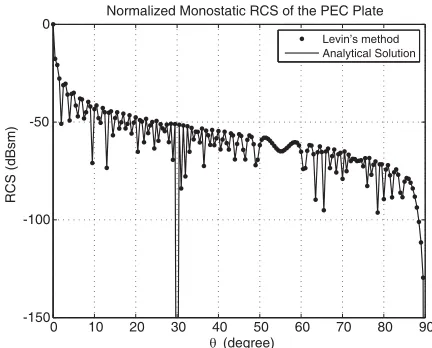
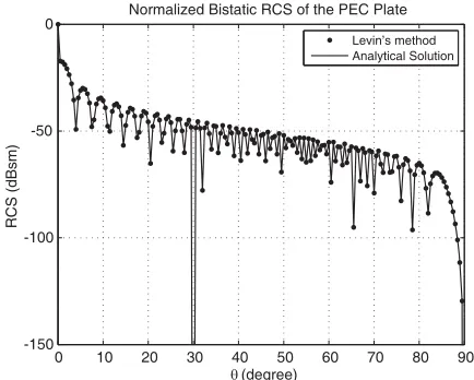
Figure 2 and Figure 3 illustrate the monostatic and bistatic RCS of a perfect electric conductor (PEC) square-shaped flat plate with side length of 100λwhich is shown in Figure 1.
y z
, i i
E H E Hs, s
x
→ → → →
Figure 1. Simulation setup for PEC plate.
0 10 20 30 40 50 60 70 80 90
-150 -100 -50 0
θ (degree)
RCS (dBsm)
Normalized Monostatic RCS of the PEC Plate
Levin’s method Analytical Solution
Figure 2. Monostatic RCS of a PEC plate.
compared with the analytical result of the physical optics integral for these problems. It can be observed from Figure 2 and Figure 3 that, the results obtained by Levin’s method perfectly match with the analytical solution, for both cases. Here, it is important to note the PEC plate is modeled by only one single patch.
0 10 20 30 40 50 60 70 80 90 -150
-100 -50 0
θ (degree)
RCS (dBsm)
Normalized Bistatic RCS of the PEC Plate
Levin’s method Analytical Solution
Figure 3. Bistatic RCS of a PEC plate.
relative error of the Levins algorithm can be attained by
Error= 1 Nangle
Nangle
i=1
σianalytic−σlevini
σanalytici
(26)
where Nangle is the number of observation angles and σanalytici and
σlevini are the RCS values at the ith observation angle computed
analytically and by Levin’s method, respectively. If the RCS values illustrated in Figure 3 are used, the relative error of the Levin’s algorithm, for the bistatic case, is obtained as 2.78×10⁻⁴ with an observation resolution of 0.5◦ (for 181 observation angles). Here, it is important to note that, due to the fact that the actual RCS values at the observation anglesθ= 30◦ andθ= 90◦are very small, these angles are discarded from the data points for a fair evaluation of the accuracy of Levin’s algorithm.
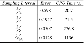
Table 1. The relative error and CPU time of brute force integration for different sampling intervals.
Sampling Interval Error CPU Time (s)
2
λ 0.598 20.7
4
λ 0.1947 71.5
8
λ 0.0507 276.8
16
λ 0.0128 1136
and 2 for double integration) by some modifications in the code. It may be observed that the brute force integration cannot reach the accuracy of Levin’s method even if the sampling interval is reduced to λ/16. Moreover, Levin’s method computes the bistatic RCS of the PEC plate in 2.03 seconds including all of the i/o processes for 181 observation angles.
In addition to the accuracy and run time analysis of Levin’s integration technique discussed above, another performance check is conducted to investigate the speed of Levin’s method for different frequencies. In this performance analysis, the bistatic RCS of a square flat plate, with a side length of 3 m, is computed at 10 different frequencies starting from 1 GHz to 10 GHz. The CPU times of each run obtained by Levin’s algorithm are recorded and compared with the ones obtained by brute force integration with a sampling interval ofλ/16. It can be observed from Figure 4 that the run time of Levin’s algorithm remains almost constant (around 2 seconds). On the other hand, the run time of brute force integration increases drastically with increasing frequency.
The performance of Levin’s method has been proved to be accurate for flat plates. However, in the previous sections it was mentioned that Levin’s method is applicable to any surface modeled as a quadrilateral. Indeed, one of the most important advantages of Levin’s method is this property. Therefore, for a complete performance check of this novel technique, further simulations are needed to be conducted on curved surfaces.
1 2 3 4 5 6 7 8 9 10 100
101 102 103 104
Frequency (GHz)
CPU Time (s)
CPU Times vs Frequency
Brute Force Integration Levin’s Method
Figure 4. Comparison of run times of Levin’s algorithm and brute force integration for different frequencies.
ο
5
= ϕ
λ
100
=
l
x
y z
θ i E
Figure 5. Simulation setup for singly curved screen.
0 10 20 30 40 50 60 70 80 90 -20
-15 -10 -5 0 5 10 15 20 25
30 Bistatic RCS of a Singly Curved Surface
θ (degrees)
RCS (dBsm)
Brute Force Integration Levin’s Method
Figure 6. Bistatic RCS of a singly curved PEC screen.
ο 6
=
α
ο 6
= β
x
y z
φ
i E
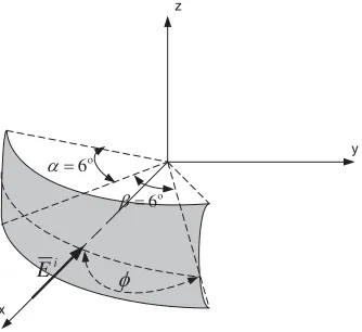
Figure 7. Simulation setup for doubly curved screen.
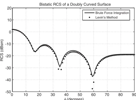
0 10 20 30 40 50 60 70 80 90 -50
-40 -30 -20 -10 0 10 20
Bistatic RCS of a Doubly Curved Surface
φ (degrees)
RCS (dBsm)
Brute Force Integration Levin’s Method
Figure 8. Bistatic RCS of a doubly curved PEC screen.
is modeled with only one quadrilateral.
These numerical simulations confirm that Levin’s method is an effective and efficient technique for the computation of the PO fields even on curved surfaces.
5. CONCLUSION
The most intricate part of RCS computation by PO is the integration part. Since PO is valid at high frequencies, the complex exponential term in the integrand of the PO integral becomes very oscillatory at high frequencies. Hence, too many sampling points are needed with the classical quadrature methods. To increase the computational efficiency of PO, a novel fast integration technique, which is called Levin’s integration method, is applied to electromagnetic scattering problems. In this method, an accurate solution can be attained for an integral on a rectangular domain by making use of only a few collocation points. The integrand is approximated by some basis functions (monomials in this study) and the integration is converted to solving a differential equation where a nonoscillatory particular solution is obtained with the help of a genius operator. In order to apply this model to arbitrary shaped objects, the surfaces of the objects are modeled by 8-noded isoparametric quadrilaterals. Then, with the help of some shape functions, the integration domain is mapped to a rectangular domain where Levin’s method is easily applicable.
integrals with rapid oscillations. Since it can be applied to curved surfaces, the number of patches used for target modeling can be decreased drastically. Hence, computational efficiency of Levin’s method is higher than the methods using planar patches to model the targets. Moreover, the complexity of the algorithm is almost of order zero with respect to frequency. That is, the number of computations and CPU time does not change with frequency. Therefore, very large facets (such as facets with a surface area of 10000λ2) may be used for target modeling. This makes Levin’s method appropriate for large targets like ships, planes and tanks.
Despite the advantages of Levin’s method, there are some drawbacks restricting the usage of it. Due to the possible singularities stated in the paper, Levin’s method cannot be applied to PO integrals at low frequencies. Since a rapid phase variation within a facet is also necessary for the application of the method, small facets are not appropriate for this technique. Thus, for some cases the geometry of a target may not be modeled precisely. Furthermore, Levin’s method is not applicable to computation of the scattered fields in the neighborhood of forward scattering region because of the same reason.
REFERENCES
1. Ludwig, A. C., “Computation of radiation patterns involving double integration,” IEEE Transactions on Antennas and Propagation, Vol. 16, No. 6, 767–769, November 1968.
2. Dos Santos, M. L. X. and N. R. Rabelo, “On the Ludwig integration algorithm for triangular subregions,” Proceedings of the IEEE, Vol. 74, No. 10, 1455–1456, October 1986.
3. Moreira, F. J. S. and A. Prata, “A self-checking predictor-corrector algorithm for efficient evaluation of reflector antenna radiation integrals,” IEEE Transactions on Antennas and Propagation, Vol. 42, No. 2, 246–254, January 1994.
4. Kobayashi, H., K. Hongo, and I. Tanaka, “Expressions of physical optics integral for smooth conducting scatterers approximated by quadratic surfaces,” Electronics and Communication in Japan, Part 1, Vol. 83, No. 7, 863–871, 2000.
5. Flinn, E. A., “A modification of Filon’s method of numerical integration,” Journal of the ACM, Vol. 7, No. 2, 181–184, April 1960.
7. Vico, F., M. Ferrando, M. Baquero, and E. Antonino, “A new 3D fast physical optics method,” IEEE Antennas and Propagation
Society International Symposium 2006, 1849–1852, July 9–14,
2006.
8. Corona, P., G. Manara, G. Pelosi, and G. Toso, “PO analysis of the scattering from polygonal flat-plate structures with dielectric inclusions,” Journal of Electromagnetic Waves and Applications, Vol. 14, 693–711, 2000.
9. Arslanagic, S., P. Meincke, E. Jorgensen, and O. Breinbjerg, “An exact line integral representation of the physical optics far field from plane PEC scatterers illuminated by Hertzian dipoles,”
Journal of Electromagnetic Waves and Applications, Vol. 17,
No. 1, 51–69, 2003.
10. Levin, D., “Procedures for computing one and two dimensional integrals of fumctions with rapid irregular oscillations,” Mathe-matics of Computation, 531–538, April 1982.
11. Kuzuoˇglu, M., “Solution of electromagnetic boundary value problems by the plane wave enriched FEM approach,”IEEE APS-URSI International Symposium, 2003.