Topics in Numerical Relativity: Solving the Initial Value Problem Using Adaptive Mesh Refinement, Examining Evolution Stability Using Spectral Methods, and Finding Apparent Horizons using a Mean Curvature--Level Set Method

(1)

ABSTRACT

LOWE, LISA L. Topics in Numerical Relativity: Solving the Initial Value Problem Using Adaptive Mesh Refinement, Examining Evolution Stability Using Spectral Methods, and Finding Apparent Horizons using a Mean Curvature–Level Set Method. (Under the direction of Associate Professor J. David Brown).

Various topics in numerical relativity will be discussed, including solving the initial

value problem using adaptive mesh refinement, examining evolution stability using spectral methods, and finding apparent horizons using a mean curvature–level set

method. We use the ADM 3+1 formalism, which separates the Einstein equations

into four constraint equations and twelve evolution equations. The four constraint equations are then transformed via a York–Lichnerowicz transverse traceless

decom-position. We give a brief discussion on variations of this decomdecom-position. We discuss

the implementation of a parallel multigrid solver with adaptive mesh refinement for solving the initial value constraint equations. Using our multigrid solver, we solve

for a new class of initial data: distorted black holes using the puncture method. The

ADM evolution equations have known instabilities. We explore the instabilities in-herent in the evolution equations with an evolution code implemented using spectral

methods with a Runge–Kutta integrator via the method of lines. An overview of

spectral methods is given. We compare the results of evolving the full ADM

evolu-tion equaevolu-tions with stability predicevolu-tions from integrating the constraint equaevolu-tions. Evolution instabilities can be contained by adding multiples of the constraints to the

evolution equations. We show how to implicitly dictate the behavior of constraint

vio-lation during an evolution by manipulating additional constraint terms. After solving for initial data or during an evolution, it is often necessary to locate the position of

the apparent horizon. We rewrite the apparent horizon equation as a surface

evolv-ing along its normal vector accordevolv-ing to the speed of the apparent horizon equation. Instead of evolving a two dimensional surface and assuming a star shaped topology,

we evolve a three dimensional surface via the level set method. This allows us to find

(2)

(3)

Topics in Numerical Relativity: Solving the Initial Value Problem Using Adaptive Mesh Refinement, Examining Evolution Stability Using Spectral Methods, and

Finding Apparent Horizons using a Mean Curvature–Level Set Method

by Lisa L. Lowe

A dissertation submitted to the Graduate Faculty of North Carolina State University

in partial fullfillment of the requirements for the Degree of

Doctor of Philosophy

Physics

Raleigh, North Carolina

2008

APPROVED BY:

Dr. John M. Blondin Dr. Gail McLaughlin

Dr. J. David Brown Dr. Stephen P. Reynolds

(4)

DEDICATION

(5)

iii

BIOGRAPHY

Lisa Lowe attended Belle Vernon Area High School in southwestern Pennsylva-nia, where she studied physics under Mr. Thomas C. Thompson Jr. She obtained

her undergraduate degree in physics from Drexel University in Philadelphia,

Penn-sylvania. At Drexel, she worked with Professor Joan M. Centrella on hydrodynamic simulations of instabilities in rapidly rotating polytrope stars [1]. Lisa completed a

co–op at the Princeton Plasma Physics Laboratory in Plainsboro, New Jersey where

she implemented a parallelization of a guiding center drift orbit integrator [2] and developed a field line tracing routine for a resistive magnetohydrodynamics code with

finite elements on unstructured meshes [3]. She attended graduate school at the North

Carolina State University in Raleigh where she worked as the head teaching assistant

for Astronomy Labs and for a semester was the Interim Manager of the Physics Tu-torial Center. At NC State, she did research in the field of numerical relativity with

Professor J. David Brown. Her research included implementing a multigrid solver

with adaptive mesh refinement [4], solving initial data for distorted black holes using the puncture method [5], investigating the stability of the Einstein equations with

spectral methods [6], and finding apparent horizons with a mean curvature flow level

(6)

ACKNOWLEDGMENTS

I would like to thank my advisor David Brown for sharing his expert knowledge with me; I only wish I could have absorbed more of it during my studies. He has

made several attempts to push me away from blind numerical experimentation

to-wards mathematical rigor and careful thought. Although I am light-years away from achieving his level of excellence, I thank him for providing the standard that I will

work toward. On a more personal level, I am grateful to have had an advisor with

an open door policy and the ability to patiently explain (sometimes repeatedly) com-plicated ideas and concepts. He and his wife Stefanie have also been great friends to

me, and they have been an endless reservoir of support for me and my family since

the day we moved into the area.

I am grateful for all the sources of funding I have received during my graduate studies. All course work was completed while being supported by a Teaching

Assis-tantship from the Physics Department at NC State. I give special thanks to Robert

Egler for supporting me in my position as Astronomy teaching assistant and head teaching assistant. A GAANN fellowship enabled me to take a break from teaching

to study for the qualifying exam while also having time to work on coding. Work

developing the multigrid solver, the spectral methods solver, and the apparent hori-zon finder was supported by Research Assistant funding from Dr. J. David Brown.

The writing of this dissertation was supported by an American Fellowship from the

American Association of University Women.

I would like to express my sincere gratitude to all of my previous advisors and

mentors, for without them I would not have had the confidence and experience

nec-essary to have achieved what I have. In particular, Joan Centrella not only paved my way into computational physics and relativity, but took me by the hand down

the path. As a freshman undergraduate, I had a work-study job doing filing and

secretarial work for the Physics department. She came by and handed me a Fortran manual and asked me if I wanted a job doing real physics. Other than offering me

invaluable experience and connections, I still often recall her words of wisdom and

(7)

v

mentor that I was fortunate to have. He not only taught me some interesting com-putational physics but also gave sage advices for confidently giving presentations in

an intense environment. Finally, I would like to thank Tom Thompson for being

an inspirational teacher. Most students either love or despise physics based on the performance of their first physics instructor. Here is no exception; if Tom had made

a different career choice, I might have as well.

Most of all, I am grateful to my family for making everything worthwhile. My mother-in-law Nada took care of my children and household during the final crunch

to finish. My daughters gave me much needed comic relief, Lena by scribbling over

my notes and yelling “No Dissertation!”, and Jana by flashing her adorable toothless grin. My husband Ivan not only provided his love and support, but also read and

(8)

LIST OF TABLES

Table 3.1 Test results confirm second order convergence of the ADM masses. . . 30

(11)

ix

LIST OF FIGURES

Figure 2.1 Extrinsic vs. Intrinsic curvature. . . 10

Figure 2.2 Diagram showing lapse and shift . . . 12

Figure 3.1 Error on a well resolved grid. . . 19

Figure 3.2 Error on a coarsely resolved grid. . . 20

Figure 3.3 A PARAMESH 3p2 grid hierarchy.. . . 21

Figure 3.4 2D contour plot of two black holes using puncture data and AMR. . 23

Figure 3.5 3D contour plot of two black holes using puncture data and AMR. . 24

Figure 3.6 Mesh for two black holes using puncture data and AMR . . . 25

Figure 3.7 Seven black holes using puncture data and AMR. . . 26

Figure 3.8 Mesh for seven black holes using puncture data and AMR . . . 27

Figure 3.9 ADM masses of distorted black holes. . . 29

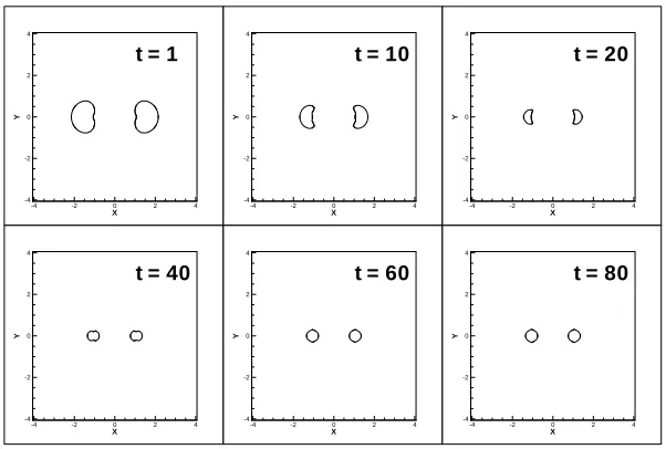
Figure 3.10 Distorted Black Holes . . . 31

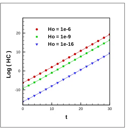
Figure 6.1 Exponential constraint growth from random initial perturbations. . . 60

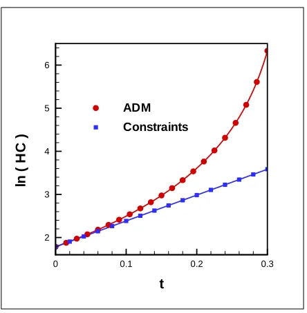
Figure 6.2 Calculated vs. analytic exponential constraint growth. . . 61

Figure 6.3 Minimum expected constraint error vs. actual constraint error. . . 62

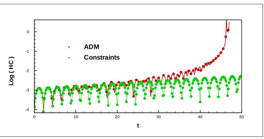
Figure 6.4 Full evolution code and constraint code until evolution code crash. . 67

Figure 9.1 Evolution of a spherical surface under mean curvature flow. . . 89

Figure 9.2 Evolution of an ellipsoidal surface under mean curvature flow. . . 89

(12)

Figure 9.4 Curvature flow of a surface starting outside horizon boundaries. . . 91

Figure 9.5 Curvature flow of a surface starting inside horizon boundaries . . . 92

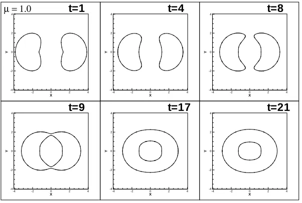
Figure 9.6 Horizons of Misner black holes with separation parameter µ= 1 . . . . 92

Figure 9.7 Horizons for a Brill wave during early evolution using AMR. . . 94

Figure 9.8 Horizons for a Brill wave during late evolution using AMR. . . 94

Figure 9.9 AMR grid structure for Brill wave test case. . . 95

Figure 9.10 Horizons for Brill wave at mid evolution using unigrid. . . 96

Figure 9.11 Horizons for Brill wave at late evolution using unigrid. . . 96

Figure 9.12 Surface evolution for Brill wave using unigrid. . . 97

Figure 9.13 Surface evolution for Brill wave using unigrid, final timestep. . . 97

Figure 9.14 Contour plots for a three Schwarzschild black hole metric. . . 98

Figure 9.15 Horizon locations for a three Schwarzschild black holes. . . 99

Figure 9.16 Surface evolution in a three Schwarzschild black hole metric. . . 99

Figure 9.17 Metric for non-time-symmetric two black hole test case. . . 102

Figure 9.18 Horizons for non-time-symmetric two black hole test case. . . 102

Figure 9.19 Contour break-up at late times for two black hole test case. . . 103

Figure 9.20 Metric for non-time-symmetric three black hole test case. . . 104

Figure 9.21 AMR grid for non-time-symmetric three black hole test case. . . 105

Figure 9.22 Surface evolution in a non-time-symmetric three black hole metric. . 106

(13)

1

Chapter 1 Introduction

Einstein published the field equations of general relativity in 1915. This caused

a shift in gravity theory from a Newtonian paradigm where objects move due to

the mysterious forces acting between them into a much simpler paradigm: objects go straight. Matter causes space to curve, and all matter travels on straight lines

in this curved space. The first exact solution to the field equations was published

shortly after the equations themselves. In 1916, Karl Schwarzschild found a

solu-tion for a spherically symmetric stasolu-tionary object. The simple idea of objects going straight becomes rather complicated due to the ‘in curved space’ caveat, so the work

of finding exact solutions is difficult. Simplifying assumptions and special

symme-tries, such as the spherical symmetry of a Schwarzschild metric, are used to find such solutions. Beyond exact solutions, analytic approximation techniques can be

used to further examine the field equations. These analytic approximations require

considerable simplifications as well. A computer is necessary to solve the Einstein equations for anything significantly complex or realistic. However, despite the advent

of powerful supercomputers and state-of-the-art numerical techniques, the two-body

problem in full general relativity (two gravitationally interacting objects), which is such a trivial scenario in the Newtonian realm, remained elusive for many years. It

was nearly a century after the Einstein field equations were first published that the

(14)

numerical relativity. Numerical relativity is the art of solving the Einstein equa-tions using a computer. The first ‘numerical relativists’ were Hahn and Lindquist in

1964 [7]. This first attempt at modeling a two black hole collision was not very

suc-cessful, and not surprisingly so, since everything about the problem was in its infancy. Computers were primitive, as was the science of numerical modeling in general. Even

the analytic side of the problem was not fully developed. At that time, the phrase

‘black hole’ did not yet exist. The term ‘black hole’ was popularized by John Wheeler in 1967. Instead, the term ‘geometrodynamics’ was used in this first numerical

rela-tivity publication. Although unsuccessful in modeling a black hole merger, Hahn and

Lindquist successfully inspired other scientists to attack the two-body problem. In 1970, Dewitt, Smarr, and Eppley published the results of a simulation that followed

two black holes as they merged into one [8].

As the fledgling science of numerical relativity struggled to take wing, the theo-retical implications of general relativity were already becoming well developed and

understood [9]. The theory had predicted the perihelion shift of Mercury and the

bending of light during an eclipse. Several experiments also confirmed the prediction

of a gravitational redshift. Furthermore, it could be shown through a rather simple calculation that moving objects should cause gravitational waves [10]. Gravitational

waves are ripples in the very fabric of spacetime. There was not a great deal of

cre-dence given to the idea of gravitational waves until the unexpected discovery of an oddly behaving pulsar by graduate student Russell Hulse in 1974 [11]. The

devia-tion from the expected intervals of radio signals from the Hulse–Taylor Binary Pulsar

could be explained by energy being dissipated as gravitational waves. This discovery implied that gravitational waves did indeed exist and thus could be detected and

stud-ied. Another branch of science was then created—gravitational wave science. The

quest to detect gravitational waves had begun, resulting in a collaboration by Caltech and MIT in 1983 to build a gravitational wave detector LIGO (Laser Interferometer

Gravitational Wave Observatory) [12, 13]. The project received funding by National

Science Foundation (NSF) in 1992, with the groundbreaking in 1996. Calibrations and improvements are still being made, with the possibility of a space-based

(15)

3

of this writing, NASA has set an earliest launch date estimate for LISA as 2018 [14]. In the 1990’s, anticipation for LIGO inspired researchers to pursue with renewed

vigor the two-body problem of general relativity. The Black Hole Binary Grand

Chal-lenge Alliance was formed and funded in 1993. The goal of the alliance was to build up numerical algorithms and infrastructure to successfully produce a three-dimensional

model of the inspiral, merger, and resulting gravitational waves of two black holes1_.

During the Grand Challenge era, great volumes of knowledge were acquired. Many computer programs were written and rigorous testbeds were developed for verifying

the accuracy and stability of algorithms [16]. Alternate mathematical representations

of the equations were formulated to enhance stability [17]. Techniques were devel-oped to handle the inherent singularities of black hole spacetimes(e.g., excision [18],

punctures [19], gauge choices [20]). On the computational front, faster, more efficient

algorithms and parallel adaptive grid infrastructure were being developed while the availability of supercomputers was becoming more widespread. By 1998, stable long

running evolutions of single black holes were possible [21], but similar success with

binary black holes still seemed a long way off. At the end of the 1990’s, many

re-searchers began to study in detail the stability issues inherent in the formulation of the Einstein equations [22]. A great deal of work was done to understand issues such

as the mathematical classification of the equations (such as hyperbolicity) and how

to formulate appropriate boundary conditions. Meanwhile, the library of numerical algorithms continued to grow. Adaptive mesh refinement, parallel processing, and

better computational approximations of equations (higher order finite differencing,

spectral methods) were becoming well developed. This new wealth of knowledge led to two simultaneous breakthroughs, both for the first time succeeding in solving the

elusive two-body problem of general relativity. The first came from the understanding

that the standard formulations of relativity were, in general, ill-suited to solve the problem at hand. Most work on the stability of formulations entailed modifications

of the usual (ADM) equations, but in 2004, work using a different formulation of the

Einstein equations (known as ‘generalized harmonic coordinates’) led to the first

sim-1

(16)

ulation of a black hole binary inspiral and merger [23, 24]. The second breakthrough surfaced as a culmination of relativity work over the years. In 2005, two research

groups were able to take a binary system through inspiral and merger via a ‘moving

puncture method’. The moving puncture method is successful by means of a modified form of the equations (BSSN), specialized gauge choices, and advanced computational

techniques. The computational technique of adaptive mesh refinement was used to

allow the resolution needed to evolve highly singular objects (punctures) [25, 26, 27] while providing the ability to place boundary conditions far from the source. Since

these successful simulations were published, researchers have been developing their

existing codes and writing new ones to run their own successful simulations using either the moving puncture or generalized harmonic method2_.

This dissertation touches on a representative sampling of the issues in numerical

relativity. Chapter 2 describes some of the necessary theoretical background including the Einstein equations and the 3+1 decomposition of the Einstein equations known

as the ADM decomposition. Chapter 3 explains the initial value problem of general

relativity. To evolve any physical system, one must start with valid initial data.

The initial data must obey the laws of physics; in our case, it must satisfy constraint equations. Chapter 4 will describe our initial value solver using multigrid and adaptive

mesh refinement calledAMRMG(Adaptive Mesh Refinement MultiGrid). The initial

data for one of the first successful binary black hole simulations was provided by

AMRMG. Chapter 5 details a new class of initial data made feasible by AMRMG:

distorted black holes using the puncture method. Chapter 6 describes the evolution

equations as they written in the ADM formalism. It explains the inherent stabilities encountered with this form, and it illustrates exponentially growing instabilities with

some numerical examples. This chapter also contains an introduction to controlling

constraint violations during an evolution. We use spectral methods to implement a constrained evolution. Spectral methods are well established computational tools, but

they are somewhat novel to the numerical relativity community. Chapter 7 explains

spectral methods as they are most commonly used in relativity and describes the

2

(17)

5

successes and problems we have encountered in implementing an evolution code using pseudospectral collocation. Chapter 8 is our publication explaining how any system,

such as the Einstein evolution equations, might be altered to control the growth of

constraint violating modes (i.e., to make the system numerically well behaved). After solving for the configuration of a certain spacetime, it is important to understand its

physical characteristics. In particular, it is useful to be able to search for horizons in

a spacetime. Chapter 9 will describe an apparent horizon finder using a method that evolves a level set according to its mean curvature or expansion flow. Chapter 10

gives a summary of the three major code projects described in this dissertation, and

(18)

Chapter 2 Equations

There is a dilemma in formulating an introductory chapter on numerical relativity.

The likely prospective audience for such a text would be either a graduate student

beginning to do research or someone already working in the field. To a veteran of the field, a lengthy explanation of the material is trivial and unnecessary. In light of

this, the spirit of the following chapter is to present the material in a way that it is

conceptually understandable to an incoming graduate student1_{. Accurate formulas,}

common notation, and useful references for further study are provided. The aim will be to allow a beginner to jump in and work without getting immediately scared off

by the imposing looking and unfamiliar math. A veteran can scan through for the

notation conventions used.

2.1 Einstein equations

A relativity dissertation is most appropriately begun with the Einstein equations,

thus, to begin we have2

Gµν = 8πTµν. (2.1)

Gµν is the Einstein tensor. It represents curvature. Tµν is the stress energy tensor.

1

In a similar vein, Miller [33] provides a brief explanation of numerical relativity for the beginner. 2

(19)

7

It represents matter. This relation is most eloquently explained by John Wheeler: “Spacetime tells mass how to move, and mass tells spacetime how to curve.” Space

is described by the metric. A metric tensor will be denoted gµν , and a metric will

be denoted3 _by _ds2 _≡_g

µνdxµdxν. The metric gives the distance between two points. The most common example is a two-dimensional flat metricds2 ₌_dx2₊_dy2_{. This is}

just the familiar Pythagorean theorem. Here are two examples.

A cylindrical metric:

gij = 

  

1 0 0

0 ρ2 ₀

0 0 1



  

(2.2)

ds2 ₌_d2_ρ₊_ρ2_d2_φ₊_dz2

The Minkowski metric:

gµν = 

     

−1 0 0 0

0 1 0 0

0 0 1 0

0 0 0 1



     

(2.3)

ds2 ₌₋_dt2₊_dx2₊_dy2₊_dz2

The cylindrical metric is purely spatial—there is no time information. For spatial

metrics, we will use Latin indices running from 1 to 3 with metric signature (+,+,+). The Minkowski Metric is a ‘spacetime’ metric—it contains information about both

space and time. For spacetime metrics, we use Greek indices running from 0 to 3.

A spacetime metric has metric signature (-,+,+,+). A metric with such signature is called a ‘pseudo-Riemannian metric’.

General relativity is a description of gravity as geometry. Mass creates curvature.

Curvature is computed from derivatives of the metric. In differential geometry, the geometry of curved space, a Riemann tensor gives us a measure of curvature. If the

3

(20)

Riemann tensor,Rµναβ, equals zero then the curvature is zero, i.e., flat. The Riemann tensor consists of the metric and its derivatives as follows:

Rµ_ναβ _≡∂αΓµ_νβ₋∂βΓµνα+ Γ µ σαΓ

σ µβ−Γ

µ σβΓ

σ

µα (2.4)

where the Christoffel symbols, Γµ_αβ, are defined as

Γµ_αβ = 1 2g

µσ₍_∂

αgβσ+∂βgασ −∂σgαβ). (2.5)

The Riemann tensor can be contracted to form the Ricci tensor

Rµν =Rσµσν, (2.6)

which can then be contracted to form the Ricci scalar, or scalar curvature

R=gµν_R

µν. (2.7)

Now we can express the Einstein tensor in terms of the Riemann tensor

Gµν =Rµν− 1

2gµνR. (2.8)

Compare the field equations of relativity (equation [2.1]) with the familiar

New-tonian equation for gravitational potential.

Gµν = 8πTµν (2.9)

∇2ψ = 4πρ (2.10)

The Newtonian theory gives the Poisson equation, a differential operator acting on the gravitational potential depending on a matter source term. Recalling that Gµν is

made up of the metric and its derivatives, one can see that the Einstein equations are

also differential equations. The matter source term is Tµν and the left hand side is a differential operator acting on the metric. In principle, we simply describe the source

term and solve the equations for the metricgµν. In practice, however, solving this set

of equations is anything but simple. As intimated in the Introduction, solving the Einstein equations is quite a complicated task, even in the absence of source terms

(21)

9

spacetimes with black holes and gravitational waves. In this dissertation, only vacuum relativity will be discussed. The equation of interest is now

Gµν = 0. (2.11)

Unlike its source free Newtonian counterpart (the Laplace equation), there is no

straightforward prescription for solving equation (2.11). Equation (2.11) is a set of ten nonlinear coupled second order partial differential equations.

2.2 ADM—The 3+1 Decomposition

It is difficult to imagine where one would start when faced with the set of equations that is equation (2.11). What one likely does is make an attempt to translate the

unfamiliar into something more routine. The Einstein tensor gives information for a

four-dimensional spacetime. We are more likely to imagine ourselves in a particular place at one time, then visualize that time is moving forward. The ADM (Arnowitt,

Deser, Misner) decomposition [34], also known as the 3+1 formalism, is a way to

create three spatial dimensions going forward in time. Using ADM allows us to do computations in this familiar way4_{. Technically, the ADM decomposition separates}

spacetime into a set (or foliation) of spacelike hypersurfaces evolving in time5_.

Doing this separation gives what is known as a Cauchy problem [36]. ‘Cauchy

problem’ basically means ‘initial value problem’. Consider the Newtonian ‘projec-tile’ initial value problem. If the initial position and momentum of an object are

known, the trajectory can be predicted for all time. In the Hamiltonian formulation

of classical mechanics, we talk about ‘q’s and p’s’ or ‘position and momentum’ as con-jugate variables. In 3+1 relativity, the ‘q’ is the metric of the spacelike hypersurface

gij6. What is the ‘p’ ? We need something that acts like a momentum. The metric

4

Although the ADM formalism turns the Einstein equations into a ‘computer ready’ type system of equations, this was not its original purpose. The ADM decomposition came about as an attempt to quantize gravity by defining a general relativistic Hamiltonian.

5

Reference [35] gives a step-by-step description on how to project the spacetime quantities of the Einstein equations into the three-dimensional hypersurfaces.

6

(22)

Figure 2.1: Extrinsic vs. Intrinsic curvature.

gij represents curvature, so what would represent the change in curvature? A brief

discussion of curvature will answer this question.

Consider the cylinder in figure 2.1. An ant crawling on the cylinder sees no

curvature. In the absence of curvature, two initially parallel lines will never intersect,

and the ant will verify that this is true on the cylinder. The type of curvature an ant sees is called ‘intrinsic curvature’. It is intrinsic to the manifold. An observer outside

of the manifold will insist that the cylinder is curved. The curvature comes about

from how the two-dimensional cylinder is embedded in the three-dimensional space of the observer. This is known as ‘extrinsic curvature’. An observer can measure how

the curvature of the cylinder changes with respect to the surrounding area by placing

an arrow normal (or orthogonal) to the surface of the cylinder and moving it around, observing how fast the arrow changes directions. Now replace the cylinder with a

three-dimensional spacelike hypersurface. The intrinsic curvature of our hypersurface

is gij, and the extrinsic curvature (our momentum-like variable) will be denoted by

Kij. Kij is defined as

Kij =− 1

2Ln(gij) (2.12)

(23)

11

to the hypersurface.

Imagine we now have a set of spacelike hypersurfaces containing the dynamical

variables gij and Kij. Each hypersurface is defined at an instant of constant time.

The dynamical variables evolve in time from one hypersurface to another. The next step is to define the trajectory needed to take a point xi _{at time} _t _{forward in time}

to t +δt. To do this we break up the time vector into components normal to the

hypersurfacenµ _{and tangent to the hypersurface} _βµ

tµ=αnµ+βµ. (2.13)

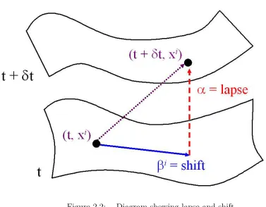
Figure 2.2 shows a diagram depicting this. The lapseα gives the information about the ‘time lapsed’ from one surface to the next, while the shift vectorβi_{tells us how the}

coordinates shift7_{. These gauge conditions are also referred to as ‘slicing conditions’.}

The spacetime is ‘sliced’ into hypersurfaces, but there is not a unique way of doing

this. The easiest thing to imagine is having a block and making horizontal slices

straight across. Each point would go directly forward in time (α = 1) and there

would be no shift in coordinates (βi _{= 0). Although this is the simplest case, it}

is usually necessary to make a more clever choice for the lapse and shift to avoid instabilities and singularities.

To summarize, in order to create an initial value formulation of relativity, the

four-dimensional spacetime equations of relativity are decomposed via the 3+1 split of the ADM formalism. The split is done by defining a foliation of spacelike hypersurfaces

and projecting the Einstein equations onto that foliation. In doing so, we obtain a

position-like quantity,gij, and a momentum-like quantity,Kij. The separation results in constraint equations and evolution equations for the dynamical variables gij and

Kij. One must solve the constraint equations to provide valid physical initial data

on the initial spacelike hypersurface (t=0). After valid initial data is specified, the evolution equations are used to evolve the data onto future hypersurfaces. To perform

an evolution, one must choose freely specifiable gauge conditions, α and βi_.

The ADM metric is expressed as

ds2 _≡γµνdxµdxν = (βaβa−α2)dt2+ 2βadxadt+gabdxadxb. (2.14)

7

(24)

Figure 2.2: Diagram showing lapse and shift

The ADM equations in their most commonly used form are:

H _≡ K2₋KijKij +R= 0 , (2.15)

Mi ≡ DjKij −DiK = 0 , (2.16)

∂⊥gij = −2αKij , (2.17)

∂⊥Kij = αKKij −2αKikKjk+αRij −DiDjα (2.18)

where∂⊥≡∂/∂t− Lβ represents the time derivative. Lβ is the Lie Derivative along

βi_{, and}_D

i is the covariant derivative. H is called the Hamiltonian constraint andM the momentum constraint. The covariant derivative for a tensorTij is defined as

DkTij =∂kTij −ΓlkiTlj −ΓlkjTil, (2.19)

and the Lie Derivative of a tensor Tij with respect to a vector field βk is

(25)

13

Chapter 3 The Initial Value Problem

Four of the ADM equations do not contain second time derivatives of the metric;

they are constraint equations. The constraints need to be solved to obtain valid initial

data which can then be evolved using the evolution equations. The Hamiltonian and momentum constraint equations are

H _≡ K2₋KijKij +R = 0 (3.1)

Mi ≡ DjKij −DiK = 0. (3.2)

The constraints in the form of equation (3.1) cannot be solved uniquely for the metric

and extrinsic curvature. Something must be done to put the equations into a standard form that can be solved uniquely. The equations are decomposed into freely

specifi-able quantities and quantities to be solved for. Section (3.1) explains the conformal

decomposition, which is a common way of accomplishing this. After the conformal decomposition we are left with a set of four nonlinear elliptic partial differential

equa-tions (PDE’s). Multigrid is one of the most efficient ways of solving an elliptic PDE.

Section 3.2 gives an introduction to our multigrid paper. Using our multigrid solver AMRMG, we have solved for a new class of initial data: distorted black holes using the puncture method. Section 3.3 gives an introduction to our paper on distorted

(26)

3.1 The Conformal Decomposition

3.1.1 Introduction

There are 12 unknowns (gij,Kij) but only four constraint equations in the initial

value problem. Something must be done in order to transform this set of equations

into a standard elliptic system of equations with a unique solution, i.e. four equations with four unknowns. There are several different ways of doing this, and perhaps

one of the most common is the York–Lichnerowicz conformal decomposition1_{. The}

conformal decomposition takes the system of 12 unknownsgij andKij and transforms

it into a new system of only four unknowns which will be labeled ψ and wa_.

Any tensor can be decomposed into a scalar multiplier times another tensor. We

call the scalar multiplier the ‘conformal factor’ and say that these tensors are

‘con-formally related’. We can decompose a tensor Cij _{into a conformal factor times a}

conformal tensor (denoted with tilde) ˜Cij_:

Cij =ψnC˜ij (3.3)

Here, the conformal factor ψ can be to any power of n. The n is chosen in such a

way that it simplifies or gives a desired form to the math in question. In the case of

the metric decomposition for the initial value equations,n is chosen to be₋4, so that

gij ₌_ψ−4_g_˜ij _and _g

ij =ψ4g˜ij.

There are further tensor manipulations that are used in the initial value

decom-position. One technique is to break up a tensor into its trace and tracefree parts. Any symmetric tensor may be decomposed in this manner. For example, we can

decompose a symmetric tensor Cij _{into its trace and tracefree part (}_Fij₎

Cij = 1 3C

k kδ

ij

+Fij. (3.4)

We can further decomposeCij _{using what is known as a transverse-traceless}

decom-position. Any trace-free symmetric tensor (likeFij_{) can be split as}

Fij =Bij + (Lw)ij (3.5)

1

(27)

15

where (Lw)ij ₌_Di_wj₊_Dj_wi − 23g

ij_D

kwk and Bij is transverse traceless (DjBij = 0 and trBij _{= 0).}

To summarize, there are some tensor manipulations that can be done to

rear-range the initial value equations. One can perform a conformal decomposition and a transverse traceless decomposition. The resulting equations differ depending on

which order these two operations are performed and which power of conformal factor

is used.

3.1.2 Conformal Transverse Traceless

The most common way of doing the initial value decomposition is the conformal

transverse traceless method. This method is performed by first doing a conformal decomposition and then performing the transverse traceless decomposition of the

tracefree part of the extrinsic curvature Kij.

The conformal metric ˜gij is defined by

gij =ψ4g˜ij (3.6)

In the following, variables with a tilde (e.g.,˜g) are conformal variables, to be raised

and lowered with the conformal metric. To simplify the momentum constraint (K

equations), first we separate Kij _{into its trace and tracefree parts. Any symmetric}

tensor can be decomposed into a trace and tracefree part.

Kij ₌_Aij ₊1 3g

ij_K _(3.7)

Now we perform a conformal decomposition of the tracefree part ofKij:

Aij ₌_ψn_A_˜ij _(3.8)

Heren can be any number, but because when n = 10 we have

DjAij =ψ −10_D_˜

jA˜ij, (3.9)

n = 10 is typically chosen as it will simplify the momentum constraint. If we let n

be any number, we have

Kij =ψnA˜ij + 1 3g

ij

(28)

Any trace-free symmetric tensor (like ˜Aij_{) can be split as}

˜

Aij _{= ˜}_Bij_{+ ( ˜}_Lw₎ij _(3.11)

where ( ˜Lw)ij _{= ˜}_Di_wj_{+ ˜}_Dj_wi − 23˜g

ij_D˜

kwk and ˜Bij is transverse traceless ( ˜DjB˜ij = 0 and tr ˜Bij _{= 0).}

So in terms of this splitting, we have

Kij =ψnB˜ij +ψn( ˜Lw)ij +1 3ψ

−₄ ˜

gijK (3.12)

The Hamiltonian constraint and momentum constraint become:

H = ₋ψ2n+8A˜abA˜ab+ 2

3K+ψ

−4_R_˜

−8ψ−5_D_˜2_ψ _(3.13)

Ma = (n+ 10)ψn+3D˜bψA˜ba+ψn+4D˜bA˜ba− 2

3D˜aK (3.14)

Ifn =₋10, we get the ‘usual’ conformal transverse traceless equations.

H = ₋ψ−12_A_˜

abA˜ab+ 2

3K+ψ

−4_R_˜

−8ψ−5_D_˜2_ψ _(3.15)

Ma = ψ

−6_D_˜ bA˜ba−

2

3D˜aK (3.16)

Usingn=₋4 also provides some simplification, and we get what will later be referred to as the ‘same sign decomposition’ (same sign as the n for the conformal inverse

metric).

H = ₋A˜abA˜ab+ 2

3K +ψ

−₄_˜

R₋8ψ−5D˜2ψ (3.17)

Ma = 6ψ −₁_˜

DbψA˜ba+ ˜DbA˜ba− 2

3D˜aK (3.18)

3.1.3 Physical Transverse Traceless

The physical transverse traceless method is when one performs a transverse

trace-less decomposition first and then use a conformal decomposition. As before, we start with

Kij ₌_Aij ₊1 3g

(29)

17

and then break upAij _{into transverse and traceless parts}

Kij =Bij + (Lw)ij +1 3g

ij

K (3.20)

whereBij _{is transverse traceless and (}_Lw₎ij ₌_Di_wj ₊_Dj_wi₋ 2 3g

ij_D kwk. Now we can do the conformal transformation

Bij ₌_ψn_B_˜ij _(3.21)

We can pick anyn, but ˜B is only transverse if we pickn =₋10. Using the conformal metric and the corresponding ˜D operators we find the relation

(Lw)ij =ψ−4_{( ˜}_Lw₎ij

(3.22)

Now we have

Kij =ψnB˜ij +ψ−4_{( ˜}_Lw₎ij

+1

3g ij

K (3.23)

The Hamiltonian constraint and momentum constraint become:

H = ₋( ˜Lw)ab( ˜Lw)ab

−2ψn+4B˜ab( ˜Lw)ab

−ψ2n+8B˜abB˜ab (3.24) +2

3K

2 ₊_ψ−4_R_˜

−8ψ−5_D_˜2_ψ _(3.25)

Ma = (n+ 10)ψn+3D˜bψB˜ab +ψn+4D˜bB˜ab + ˜Db( ˜Lw) b

a (3.26)

+6

ψD˜bψ( ˜Lw)

b a−

2

3D˜aK (3.27)

If n = ₋10, (and ˜B is transverse), we get ‘the usual’ physical transverse traceless

equations:

H = ₋( ˜Lw)ab( ˜Lw)ab

−2ψ−6_B_˜_{ab( ˜}_Lw₎ab

−ψ−12_B_˜

abB˜ab (3.28)

+2

3K

2₊_ψ−₄_˜

R₋8ψ−₅_˜

D2_ψ _(3.29)

Ma = D˜b( ˜Lw)ba+ 6

ψD˜bψ( ˜Lw)

b a−

2

3D˜aK (3.30)

3.1.4 Summary

The initial value equations are transformed by using conformal decomposition

(30)

is the conformal transverse traceless decomposition. After a conformal transverse traceless decomposition, the initial value equations are

H = ₋ψ−₁₂_˜

AabA˜ab+ 2

3K+ψ

−₄_˜

R₋8ψ−₅_˜

D2_ψ _(3.31)

Ma = ψ

−₆_˜

DbA˜ba− 2

3D˜aK. (3.32)

Often the initial extrinsic curvature is chosen to be zero (this is called ‘a moment of time symmetry’). This means that the momentum constraint is automatically

satisfied and the Hamiltonian constraint reduces to

H =ψ−4_R_˜

−8ψ−5_D_˜2_ψ. _(3.33)

3.2 AMR Multigrid

The Hamiltonian constraint is a nonlinear elliptic equation and must be solved

numerically. Methods for solving elliptic systems of equations can be classified as

direct or iterative. Gaussian elimination is an example of a direct solver. Direct

solvers require a tremendous amount of storage, usually of order N3, where N is

the number of grid points. Iterative methods generally only need storage of order

N. In numerical relativity, we need to store a grid large enough to encompass a

vast amount of space. We also need high resolution for accuracy. The memory required for such a large, well resolved grid excludes the possibility for employing

direct solvers, and iterative methods must be used. Usually, an iterative method

known as ‘relaxation’ (such as Jacobi or Gauss–Seidel) is used. These methods are slow to converge and their performance degrades with finer grids. For a grid of N

points, with grid resolutionh =O(1/N), the speed of convergence goes to zero as h

goes to zero.

This slow rate of convergence can be explained by examining the error in terms

of frequency and wavelengths. Error can be decomposed into wavelengths. Iterative

methods work by ‘smoothing out’ the error via a relaxation scheme. A typical relax-ation operator ‘sweeps’ over the grid, updating each point by a weighted average of

(31)

19

Figure 3.1: With a well resolved grid, there is little difference between values of the function at neighboring grid points and relaxation does not decrease the error efficiently.

resolved grid (many grid points). With a well resolved grid, there is little difference

between values of the function at neighboring grid points and relaxation does not

decrease the error efficiently. If the error already appears smooth (in the perspective

of each grid point), there is no significant improvement with successive relaxation sweeps, and this results in a slow convergence rate. If we put the same function as

in figure 3.1 on a coarse grid as in figure 3.2, the error is apparent and can be easily

diminished through relaxation. It can be seen in figures 3.1 and 3.2 that coarse grids can be better for eliminating certain wavelengths of error, but a coarse grid cannot

be used for solving a detailed problem. Multigrid uses a series of coarse and fine

grids to smooth the error at all frequencies. The general idea of multigrid is to put a problem on a fine grid with a trial solution and use a relaxation operator damp the

high frequency error. Then we restrict the data to a coarser grid and relax again,

damping the low frequency error. Then we can prolong the solution back onto the finer grid for a final solution2_.

Even with a memory efficient iterative method, the resources needed to solve

a three-dimensional relativity problem can be prohibitive. Great detail (via a great many grid points) is needed to resolve sources such as black holes. In order to capture

2

(32)

Figure 3.2: If we put a function on a coarse grid, the error is apparent and can be easily diminished through relaxation.

gravitational waves and ensure accurate boundary conditions, a very large domain is needed. It is not computationally possible to use high resolution everywhere for such

an enormous three-dimensional grid. Adaptive mesh refinement (AMR) is a way of

making a grid that has high resolution only where necessary. The disparity in length

scales in general relativity makes AMR essential. Gravitational wave length scales can be 100 times the length of a source.

AMR saves a great deal of computational resources by reducing the number of grid

points needed, but the problem is still very intensive. The problem must be solved on

large computers using parallel algorithms. We use a package called PARAMESH to

handle the parallel infrastructure and communications in our multigrid code [39, 40]3_.

An AMR grid is established by refining parts of the grid with a relative truncation error higher than a specified tolerance. In the testing process, sometimes it is more

instructive to have a fixed grid. Figure 3.3 shows an example of a grid that uses fixed

mesh refinement (FMR). In this case, a certain grid structure will be referred to as an ‘XpY’ or ‘X plus Y’ grid. This means thatPARAMESHhas refined X times for its base grid, and then has Y more refined grids on top of that. Figure 3.3 shows a ‘3p2’ grid

3

(33)

21

Figure 3.3: A PARAMESH 3p2 grid hierarchy. The Multigrid solver will cycle over

the highlighted levels.

and its underlying grid hierarchy. The Multigrid solver will cycle over the highlighted levels. Some multigrid methods, given a final grid like the top of figure 3.3, will begin

with an initial solution and perform relaxation along the entire top level, and then

restrict down to the next level also relaxing the error along this entire next level, and so on. This is known as FAC, for Fast Adaptive Composite grid [41]. Our multigrid

does not use FAC, rather it cycles only over the highlighted portion of figure 3.3,

beginning with only the highest resolution part of the grid (the highlighted part of the top level in figure 3.3), restricting the data to the blocks immediately underneath,

then performing relaxation on the next highest resolution part of the grid, and so on.

This is known as MLAT, or Multi Level Adaptive Technique [42]. FAC may have an advantage of providing smoother solutions, but the MLAT approach saves a great

deal of time and space by only defining and cycling over necessary portions of the

grid.

Chapter 4 is the paper that explains the specifics of our codeAMRMG(Adaptive

Mesh Refinement Multigrid) in detail. Because of limited space, we were not able to

show many interesting figures of test cases in the paper, so a few are included here.

Recall the Hamiltonian constraint equation

H =₋ψ−12A˜abA˜ab+ 2

3K+ψ

−₄_˜

R₋8ψ−5D˜2ψ. (3.34)

Given a conformal metric ˜gij and extrinsic curvature4 K˜ij, the multigrid code solves

4

(34)

the Hamiltonian constraint for the conformal factorψ. Initial data with an arbitrary number of black holes can be generated using what is known as ‘the puncture method’,

which is described in further detail in the next section. The puncture method

sepa-rates the conformal factor into singular and nonsingular parts as ψ =u+ _2rm. What is shown in the graphs is u, the nonsingular part of the metric. Figures 3.4 and 3.5

show contour plots ofufor initial data with two equal mass black holes, and figure 3.6

shows the corresponding AMR grid structure as determined adaptively byAMRMG.

To further illustrate the utility of adaptive mesh refinement, figures 3.7 and 3.8 show

initial data for seven black holes of various position, mass, and momentum and its

corresponding mesh. All data sets are three-dimensional (3D); the plots show a 2D cut of the data taken at x= 0 for the two black hole case and atz = 0 for the seven

black hole case.

3.3 Distorted Black Holes

A distorted black hole is a black hole with the addition of some gravitational waves. It is an attempt to create more realistic, astrophysically relevant initial data.

A distorted black hole metric may mimic a spacetime directly following the merger of

two black holes. The first distorted black hole metric in axisymmetry was proposed by Bernstein, et. al. [43]. This metric was subsequently modified for the general,

non-symmetric case [44]. The black hole boundary condition was implemented by

using an isometry condition. We have adapted the problem so that there does not have to be an isometry, but rather we use the puncture method to implement the

inner boundary conditions [5]. The difficulty lies then with having enough resolution

around the puncture, which makes our AMR very useful. Also, by using the puncture method, one can have multiple black holes, whereas this is not possible using isometry.

A distorted black hole metric starts out as the metric for a Brill wave [45], i.e.,

strong gravitational waves:

ds2 ₌_ψ4_[_e2q₍_dr2₊_r2_dθ2_{) +}_r2_sin2_{θ dφ}2_] _, _(3.35)

(35)

23

(36)

(37)

25

(38)

(39)

27

(40)

where q is a specified function of the spatial coordinates and ψ is the conformal

factor. We also restrict the data to a moment of time symmetry so that K = 0 and

the momentum constraints are satisfied. The Hamiltonian constraint is then

˜

∇2ψ₋ 1

8Rψ˜ = 0 , (3.36)

where ˜_∇2 _{and ˜}_R _{are the Laplacian and scalar curvature of the conformal metric}

˜

gij, defined by gij = ψ4g˜ij. The outer boundary condition is the ordinary Robin condition [∂(rψ₋r)/∂r = 0 as r _{→ ∞}]. This initial data so far presented gives a

Brill wave. To add a black hole, we must impose ‘inner boundary conditions’, which

are boundary conditions indicating where the black holes are. Bernstein, et. al. [43] used an isometry condition. Isometric means symmetric under reflections about the

black hole throat. To implement this, they choose a function q that satisfies an

isometry condition. Instead of using isometry for the black hole boundary condition,

we use a puncture. The puncture method [19] is a way of making a black hole inner boundary condition by imposing the conformal factor to be in the form ofψ =u+m

2r. This is inserted into the Hamiltonian constraint (3.36) to obtain an elliptic equation

in u:

˜

∇2u₋ 1

8Ru˜ =

m

16rR .˜ (3.37)

For certain choices of parameters in the functionq, our data sets are theoretically

equivalent to those of Brandt et. al. [44]. To verify the equivalence (and thus validity) of our puncture data, we set the required parameters (see details in chapter 5) to get

equivalent data sets, and compared our calculated ADM masses with those in [44].

We produced a figure equivalent to figure 3 of [44] and compared the two figures, finding them visually identical. Figure 3.9 shows our data for the ADM masses. We

also include the data for the ADM masses at the punctures. For isometric data sets,

the ADM mass at infinity and the ADM mass at the puncture (which is at conformal infinity) should be equal. Note that in the figure the two ADM masses are not exactly

equal. We have verified that at higher resolutions the values for the ADM masses

approach equality.

By using the puncture method, we can create distorted black hole initial data sets

(41)

29

(42)

of initial data by using parameters different from those resulting in isometry. Since these are original data sets, we need some check for validity other than comparison.

As a check for the validity of our data, we performed convergence tests of the ADM

masses. Table 3.1 shows the results of a test that keeps the outer boundary fixed and increases the grid resolution. The convergence rate confirms second order convergence

of the ADM masses. Table 3.2 shows the results of a test that kept a fixed resolution

while increasing the outer boundary. The test shows that the ADM masses do not vary greatly with outer boundary location.

Table 3.1: The results of a test that keeps the outer boundary fixed and increases the grid resolution. Column A is the ADM Mass at Infinity and B is the ADM Mass of the puncture. Columns C and D show the difference in ADM masses between the value at the same row and the value at the next higher resolution. Columns E and F divide the difference value with the value at the next highest resolution to obtain a convergence rate. The convergence rate confirms second order convergence of the ADM masses.

Type Convergence Data of the ADM Masses

of for a Fixed Outer Boundary

Grid A B C D E F

3p2 2.27354 2.31592 0.04107 0.08214 3.4600 3.4600 4p2 2.21985 2.23378 0.01187 0.02374 3.9699 3.9699 5p2 2.20648 2.21004 0.00299 0.00598

6p2 2.20317 2.20406

Table 3.2: The results of a test keeping a fixed resolution while increasing the outer boundary. The test shows that the ADM masses do not vary greatly with outer boundary location.

Type Convergence Data of the ADM Masses

of for a Fixed Resolution

Grid ADM Mass at Infinity ADM Mass at Puncture

5p3 2.206455 2.210016

5p4 2.206445 2.210016

(43)

31

(44)

Chapter 4 Multigrid elliptic equation solver

with adaptive mesh refinement

J. David Brown and Lisa L. Lowe

(45)

33

Multigrid elliptic equation solver with adaptive

mesh refinement

J. David Brown, Lisa L. Lowe*

Department of Physics, North Carolina State University, Raleigh, NC 27695, USA Received 24 November 2004; received in revised form 9 March 2005; accepted 18 March 2005

Available online 25 May 2005

Abstract

In this paper, we describe in detail the computational algorithm used by our parallel multigrid elliptic equation sol-ver with adaptive mesh refinement. Our code uses truncation error estimates to adaptively refine the grid as part of the solution process. The presentation includes a discussion of the orders of accuracy that we use for prolongation and restriction operators to ensure second order accurate results and to minimize computational work. Code tests are pre-sented that confirm the overall second order accuracy and demonstrate the savings in computational resources provided by adaptive mesh refinement.

1. Introduction

Elliptic equations appear throughout engineering, science, and mathematics. Our primary interest is in elliptic problems that arise in the context of numerical relativity. Currently, the field of numerical relativity is being driven by rapid progress on the experimental front. There are several ground-based gravitational wave detectors in operation today, and their sensitivities are quickly approaching a level at which interest-ing science can be done. There are also plans for a space-based gravitational wave detector, LISA, to be launched around 2012. The scientific payoff of these instruments will depend largely on our ability to the-oretically predict and explain the observed signals. For both ground-based and space-based gravitational wave detectors, the most common and strongest signals are expected to come from colliding black holes. Thus, much of the numerical relativity community has directed its efforts toward modeling binary black hole systems.

*_{Corresponding author. Tel.: +1 919 515 4196.}

E-mail address:[email protected](L.L. Lowe).

Journal of Computational Physics 209 (2005) 582–598

(46)

When black holes spiral together and collide, they generate gravitational waves. The black hole ‘‘source’’ region has a length scale of GM/c2_{, where} _G_{is Newton}

s constant, Mis the total mass of the two black holes, andcis the speed of light. The gravitational waves produced by the source have a length scale up to100GM/c2. Herein lies one of the challenges of modeling binary black hole sys-tems with finite difference methods. The source region requires grid zones of size[0.01GM/c2_to

accu-rately capture the details of the black holesinteraction, while the extent of the grid needs to be several hundredGM/c2to accurately capture the details of the gravitational wave signal. Many research groups in numerical relativity are starting to use adaptive mesh refinement (AMR) techniques to deal with this discrepancy in length scales [1–11]. With AMR the grid resolution is allowed to vary across the com-putational domain so that comcom-putational resources can be concentrated where they are most needed. For the binary black hole problem, we need a high resolution region to cover the small-scale detail of the source, but the gravitational waves far from the source can be modeled with sufficient accuracy using a much lower resolution grid.

Elliptic equations occur in several contexts in numerical relativity. Einsteins theory of gravity is a system of partial differential equations consisting of four constraint equations and a set of evolution equations (see for example[12]). The constraint equations restrict the data at each time step so in particular the initial data cannot be chosen freely. With suitable assumptions about the nature of the initial data, the constraint equa-tions can be written as an elliptic system[13].

Having solved the constraints for the initial data, those data are evolved forward in time by the evolution equations. At an analytical level, the evolution equations guarantee that the constraint equations will tinue to be satisfied. However, in numerical modeling, numerical errors will introduce violations of the con-straints. These violations can be disastrous because the evolution equations admit unphysical, constraint violating solutions that grow exponentially[14–17]. One possible strategy for preventing this disaster is to impose the constraints during the evolution, which means solving the elliptic constraint equations after each time step[18–20].

Elliptic equations also arise in numerical relativity when one is faced with choosing a coordinate system. In Einsteins theory the coordinate system must be chosen dynamically as the gravitational field evolves for-ward in time. The choice of coordinate system can have a dramatic effect on the performance of a numerical relativity code. Researchers have developed many different strategies for choosing a coordinate system. Some of these strategies require the solution of elliptic, parabolic or hyperbolic equations, and some involve algebraic conditions. Some researchers feel that the elliptic conditions might be best, but the cost of solving elliptic equations at each time step has made the other choices more practical and more popular.

In the numerical relativity community we need the capability of solving elliptic equations quickly on adaptive, non-uniform grids. No doubt this same need exists in other areas of science and applied mathematics.

Multigrid methods originated in the 1960s with the work of Fedorenko and Bakhvalov[21–23]. They were further developed in the 1970s by Brandt[24,25], and are now the preferred methods for solving ellip-tic partial differential equations. The advantage of multigrid is its speed – multigrid algorithms only require orderN3_{operations to solve an elliptic equation, where}_N3_{is the number of grid points. In this paper, we}

describe our code, AMRMG, which solves nonlinear elliptic equations using multigrid methods with adap-tive mesh refinement. The idea of combining multigrid with AMR is not new[24–27], although there are a number of features of our code that distinguish it from the discussions we have seen. In particular, AMRMG uses cell-centered data, as opposed to node centered data. AMRMG uses the full approximation storage (FAS) algorithm, and therefore is not restricted to linear elliptic equations. AMRMG uses the Paramesh package to implement parallelization and to organize the multigrid structure[28,29]. In[30], we used AMRMG to solve numerically for distorted black hole initial data.

(47)

35

well, and in principle AMRMG can be modified to solve any nonlinear equation. The equations of current interest for us are semi-linear, therefore we have not tested AMRMG on any fully nonlinear systems.

In this paper, we describe the algorithm behind AMRMG in detail. In Section 2, we present the overall conceptual framework behind our code, and discuss some of the choices made in its development. Section 3 is devoted to a discussion of guard cell filling, which determines the coupling between fine and coarse grid regions. In Section 4, we review the FAS algorithm and in Section 5, we discuss in detail the restriction and prolongation operators used by AMRMG. In Section 6, we describe the calculation of the relative trunca-tion error and how it is used to control the grid structure. Sectrunca-tion 7 contains the results of a number of code tests involving the calculation of initial data for numerical relativity.

2. Multigrid with AMR

The simplest technique for solving an elliptic problem is relaxation. The equation (or system of equa-tions) is written in discrete form asfi(/) =gi(/), whereilabels the grid points and/idenotes the numerical

solution. A ‘‘relaxation sweep’’ consists of refining the approximate solution/old

i by solving the system

fi(/new) =gi(/old) for /newi . [In the simplest case f is the identity and relaxation is written as

/newi ¼gið/

old

Þ.] The success of the relaxation method depends on how the finite difference equations are split into a left-hand sidefi(/) and a right-hand sidegi(/). When relaxation does work, it is slow to

con-verge. In particular the long wavelength features of the solution must slowly ‘‘diffuse’’ across the grid with successive relaxation sweeps.

To solve a problem with multigrid methods we introduce a hierarchy of grids with different resolutions. For the moment, consider the case in which we seek the numerical solution of an elliptic equation on a uni-form grid of sizeN3that covers the entire computational domain. We introduce grids of size (N/2)3, (N/4)3, etc., each covering the computational domain. On each grid the finite difference equation, or an associated equation, is solved by relaxation. The equations to be solved on each multigrid level are discussed in Section 4. For now, we simply note that the equations are chosen so that relaxation on the coarse grids quickly captures the long wavelength features of the solution. Relaxation on the fine grids captures the short wave-length features. The grids in the multigrid hierarchy communicate with one another through restriction and prolongation operators. Restriction takes data on a grid in the hierarchy and restricts it to the next coarsest grid. Prolongation takes data on a grid in the hierarchy and interpolates it onto the next finest grid. Dif-ferent multigrid algorithms use difDif-ferent sequences of grids in solving elliptic problems, but the most basic sequence is the V-cycle. In a multigrid V-cycle one starts with the finest grid, steps down the grid hierarchy to the coarsest grid, then steps back up to the finest grid.

In the context of a time-dependent problem, adaptive mesh refinement (AMR) means that the grid struc-ture adapts in time to meet the changing demands as the fields evolve. In the context of an elliptic (time-independent) problem, AMR means that the grid structure is determined adaptively, as part of the solution process, in an attempt to minimize numerical errors.

We use the Paramesh package to organize the grid structure for our code. Paramesh covers the com-putational domain with blocks of data of varying spatial resolution. These blocks form a tree data-structure. They are logically Cartesian, consisting of a fixed number of cells. We typically use 83 _cells

for each block.Fig. 1shows an example one-dimensional grid. The numbers in that figure indicate the resolution level, and the letters denote blocks. At the base of the tree structure is a single block, labeled 1A. Paramesh refines blocks by bisection in each coordinate direction. In this one-dimensional example block 1A is refined into two blocks, 2A and 2B. Since each data block contains the same number of cells, level 2 has twice the resolution as level 1. Using Paramesh terminology, block 1A is the ‘‘parent’’ of blocks 2A and 2B, and blocks 2A and 2B are the ‘‘children’’ of block 1A. InFig. 1Paramesh has

(48)

also refined blocks 2A and 2B to create blocks 3A, 3B, 3C and 3D. Further refinements yield the non-uniform grid shown in the figure. Paramesh always creates grid structures in which adjacent blocks

refinement levels differ by no more than one.

Our first task is to decide how to carry out a basic multigrid V-cycle on a non-uniform grid structure. There are two natural approaches. The first approach is the fast adaptive composite grid method (FAC) developed by McCormick[31]. In this approach, the relaxation sweeps extend across the entire computa-tional domain, and one defines the succession of multigrid levels by restricting the highest resolution sub-grid to the next lower resolution. As an example based onFig. 1, we let the top multigrid level consist of blocks 4A–5A–5B–5C–5D–4D–3C–4E–4F. After carrying out a series of relaxation sweeps on this non– uniform grid, we step down the multigrid V-cycle by restricting the data in blocks 5A–5B–5C–5D to res-olution level 4. Thus, the next multigrid level is defined by blocks 4A–4B–4C–4D–3C–4E–4F. After relaxing on this grid, we restrict the resolution level 4 blocks to resolution level 3. This defines the next multigrid level as 3A–3B–3C–3D. We can continue in this fashion to define a complete hierarchy of multigrid levels, each covering the entire computational domain.

The second approach, the one we use for AMRMG, is to define the grids in the multigrid hierarchy to coincide with the different resolution levels. This is the original multi-level adaptive technique (MLAT) pro-posed by Brandt[25,32]. As an example based onFig. 1, the top multigrid level consists of all blocks at resolution level 5, namely, 5A–5B–5C–5D. After carrying out a series of relaxation sweeps on the level 5 blocks, we restrict that data to level 4. Then the next multigrid level consists of blocks 4A–4B–4C–4D– 4E–4F. After relaxing on these blocks we restrict the resolution level 4 data to resolution level 3. Then the next multigrid level consists of the level 3 blocks 3A–3B–3C–3D. We continue in this fashion to define a complete multigrid hierarchy.

We have built and tested a one-dimensional multigrid code based on the FAC approach. That code works quite well. However, the MLAT approach appeared to us to be more straightforward to implement in a three-dimensional code based on Paramesh. For this reason AMRMG defines the levels in the multi-grid hierarchy by resolution. Apart from the issue of implementation, the MLAT approach has an advan-tage in solving problems in which only a small region of the computational domain requires high resolution. With the FAC approach, in which relaxation always extends across the entire computational domain, a lot of unnecessary computational effort can be expended on relaxation in the low resolution re-gions. On the other hand, the FAC approach has the advantage over MLAT in maintaining a tighter cou-pling between regions of different resolutions. For example, for the grid shown inFig. 1, the data in blocks 4A and 4D effectively provide boundary conditions for relaxation in blocks 5A through 5D. With FAC,

A B C D E F

A B C D

A B

A

A B C D

2 3 4 5

1

Fig. 1. Example of a one-dimensional grid structure. The numbers on the left denote the resolution level, and the letters label blocks of data.