Topology and Geometry of Sensor Networks: A Distributed Computing Approach.

(1)

ABSTRACT

CHINTAKUNTA, HARISH KUMAR. Topology and Geometry of Sensor Networks: A Distributed Computing Approach. (Under the direction of Dr. Hamid Krim.)

This dissertation is guided by two important questions; 1) What is the minimal information required to perform a ceratin task?, and likewise, 2) what tasks may be performed given certain information?

(2)

c

(3)

Topology and Geometry of Sensor Networks: A Distributed Computing Approach

by

Harish Kumar Chintakunta

A dissertation submitted to the Graduate Faculty of North Carolina State University

in partial fulﬁllment of the requirements for the Degree of

Doctor of Philosophy

Electrical Engineering

Raleigh, North Carolina

2013

APPROVED BY:

Dr. Huaiyu Dai Dr. Wenye Wang

Dr. Amadeo Hamid Krim

(4)

DEDICATION

(5)

BIOGRAPHY

(6)

ACKNOWLEDGEMENTS

I want to thank my adviser Dr. Hamid Krim for his guidance which made this dis-sertation possible. He played a big part in shaping my philosophy of Engineering, and introduced me to the joy of exploring and applying new mathematical theories to engi-neering problems. I also want to thank all my committee members, Dr. Huaiyu Dai, Dr. Amassa Fauntleroy, and Dr. Wenye Wang for their continuous support and advise, and North Carolina State University for ﬁnancially supporting me through all these years.

Perhaps the most important part of my experience pursuing my degree, is my inter-action and numerous discussions with my lab mates and colleagues. Although this is my dissertation, I feel like this is more of a group eﬀort. I would like to convey my deepest gratitude to all my colleagues, Scott Clouse, Jennifer Gamble, Dr. Athanasios Gentimis, Sheng Yi, Xiao Bian, Tian Wang, Adam Wilkerson and Shun Miao.

(7)

LIST OF TABLES

Table 3.1 Finding Diameter Nodes (left) and Boundary Nodes (right) . . . . 35

Table 3.2 contractibility of the boundary . . . 39

Table 3.3 Algorithm for Localizing Worm Holes . . . 51

Table 4.1 Distributed algorithm to compute maximum . . . 72

Table 4.2 Distributed algorithm for computing a spanning tree . . . 73

Table 4.3 Computing integral of a harmonic on a tree . . . 74

Table 5.1 Algorithm for computing the α−shape. . . 85

Table 6.1 Algorithm for computing local coordinates μi at vi . . . 103

Table 6.2 Algorithm for computing RDT(G) at node i . . . 103

(12)

LIST OF FIGURES

Figure 2.1 Homotopy Equivalent Spaces . . . 10

Figure 2.2 Examples of simplices . . . 10

Figure 2.3 Simplicial complex representing a topological space . . . 10

Figure 2.4 Homologous cycles . . . 20

Figure 3.1 Rips complex as an approximation to ˇCech complex . . . 29

Figure 3.2 Coverage hole missed by a Rips complex . . . 29

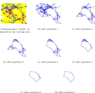
Figure 3.3 Topology preserving partitioning . . . 39

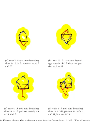
Figure 3.4 cases for boundary nodes . . . 40

Figure 3.5 Figure illustrating the simple case for assessing complexity . . . . 45

Figure 3.6 complexity for localizing holes-1 . . . 45

Figure 3.7 complexity for localizing holes-2 . . . 45

Figure 3.8 Illustration of “divide-and-conquer” algorithm . . . 46

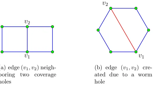
Figure 3.9 Combinatorial similarity between coverage and worm holes . . . . 47

Figure 3.10 Distinguishing coverage and worm holes . . . 50

Figure 3.11 Exceptions for heuristic to classify coverage and worm holes . . . 52

Figure 3.12 simulations on classifying coverage and worm holes . . . 52

Figure 3.13 Worm Hole Localization . . . 54

Figure 3.14 Exception for worm hole localization . . . 54

Figure 4.1 non-contractible cycles at an intermediate stage . . . 65

Figure 4.2 Illustration of distributed homology computation . . . 67

Figure 4.3 Illustration of ﬁrst step in the heuristic . . . 69

Figure 4.4 Illustration of second step in the heuristic . . . 69

(13)

Figure 5.1 Distributed computation of α−shape . . . 84

Figure 5.2 Simulation of α−shape compution . . . 86

Figure 5.3 Homotopy collapse of an edge into an adjacent 2-simplex . . . 86

Figure 5.4 Examples of the triangle setsTerc/2 and Teπ/2. . . 90

Figure 5.5 Constructions for Lemmas . . . 90

Figure 5.6 homotopy equivalence betweenArc/2(V) and DCˇrc/2(V). . . 91

Figure 6.1 Active contour approximating systematic failure . . . 99

Figure 6.2 Exception where active contour is not appropriate . . . 99

Figure 6.3 Triangulation using neighboring information . . . 102

Figure 6.4 Illustration of local coordinates . . . 102

Figure 6.5 1-skeleton of alpha complex and its boundary . . . 105

Figure 6.6 Dividing a connected component in ∂(RDT(G)) . . . 105

Figure 6.7 Construction for computing speed locally . . . 111

Figure 6.8 Robustness of the velocity estimation . . . 112

Figure 6.9 A snap shot of systematic failure and its detection . . . 114

(14)

Chapter 1 Introduction

The infrastructure of computing systems is rapidly transitioning from centralized sys-tems to distributed and pervasive syssys-tems. A very important class of such syssys-tems are sensor networks which ﬁnd applications in areas including environmental monitoring, health care and military operations [1]. A unifying theme of many of these problems is to glean consensus information by systematically combining the data collected at indi-vidual nodes, in accordance to the structure of the network. The consensus information thus obtained characterizes the network, or the data in the network as a whole, and better represents the underlying phenomenon than which can be inferred from the data at individual nodes. This reveals the fundamental nature of sensor networks, in which global patterns emerge from simple interactions between nodes.

From an engineering perspective, the fundamental challenge in sensor network appli-cations is to cope with the limited resources; a limited communication capability of nodes, i.e. nodes can only communicate with their neighbors, with limited power and limited memory. Furthermore, sensor networks are often deployed in unaccessible locations and environments where maintenance is impractical; this makes careful use of exhaustible resources such as power, imperative.

(15)

certain task. Owing to the limited power and communication capabilities, we are moti-vated to develop distributed algorithms. Although our motivation stems from challenges in sensor networks, distributed algorithms are very important even in high speed cen-tralized computing, as illustrated by ubiquitous multi-core processors, graphic processing units and massively parallel architecture of super computers.

The information which may be easily obtained in sensor networks, is for each node to know its neighboring nodes. Two nodes are neighboring nodes if they can communicate with each other. This is equivalent to having a distributed representation of the com-munication graph. With limited comcom-munication between the nodes, we may also obtain the higher order cliques in the graph, and the sub-cliques through which they connect to other cliques.

We observe that many tasks in sensor networks may alternatively be stated in topo-logical terms. The tasks of detection and localization of coverage holes and worm holes are two such examples. The combinatorial information mentioned above is sufficient to compute topological invariants, and is the subject of Algebraic Topology. We give a brief introduction to Algebraic Topology in Chapter 2 and employ this theory to develop dis-tributed algorithms to detect and localize coverage and worm holes. We emphasize that this is the first work which simultaneously solves both problems, supporting our thesis that algebraic topology offers a general framework for topological analysis in sensor net-works.

(16)

any holes in the process, to pursue the detection of holes in each. By repeating the above steps, we narrow down the location of the coverage hole. This is our “divide and con-quer” strategy, explained in detail in Chapter 3. We explain in Chapter 3, the nature of similarity of a worm-hole to a coverage hole, and how we may extend the above algorithm to detect and localize a worm-hole.

The success of the above algorithm in locating the holes led us to investigate another related problem: counting the number of holes. The knowledge of the exact number of holes can be very useful in assessing the overall quality of coverage. Locating the nodes surrounding the holes only required us to verify the non-triviality of the first ho-mology. However, counting the number of holes requires us to compute the rank of the first homology. Furthermore, computing a cycle around each hole which can serve as a unique identifier is equivalent to computing generators for the first homology. In addi-tion, computation of homology spaces and their generators has received much attention in computational homology due to numerous applications. The existing algorithms in the literature are either centralized, or utilize parallel processors with shared memory. This furthers our motivation for developing completely distributed algorithms for computing homology spaces.

In Chapter 4, we present a distributed algorithm to compute the first homology, and demonstrate its application in sensor networks. The efficacy of the algorithm relies on the following facts: 1) elements in null space of first order Laplacian, also called harmonics, provide a simple and efficient way to identify cycles which do not surround any holes, and 2) we can efficiently compute all the cycles in the graph.

(17)

the boundary.

More generally, many applications call for detecting and tracking the boundary of a dynamically varying space of interest [22] [15]. We would expect any algorithm perform-ing this task to include the followperform-ing important properties: 1) the boundary output is geometrically close to the actual boundary, and 2) the interior of the boundary is topo-logically faithful to the original space. It is often the case that we are only given random samples from the space. We may then reconstruct the space by ﬁrst placing balls of a certain radius around these points, and then by taking the union of these balls.

In Chapter 5, we start with the assumption that the union of the balls described above is a good approximation to the space of interest. Note that in case of sensor net-works, for example, this is by design. We focus our work on a set of points in a plane. A failure in the nodes is caused by a spatially propagating phenomenon, and our aim is to track its boundary nodes. In this case, we construct a space by taking the union of balls of radius rc/2 around each node, where rc is its radius of communication. The

radius of communication is the distance within which two nodes can communicate with each other. The problem may also be viewed as one of computing the boundary of a set of points, provided with some geometric information. The decision of whether a line segment joining two points (an edge in case of a network) lies on the boundary, may be locally made by constructing an associatedα−shape.

Given a set of points S in a plane, the α−shape introduced in [23] gives a gener-alization of the convex hull of S, and an intuitive deﬁnition for the shape of points. More importantly, anα−shape is the boundary of an alpha complex, which has the same topology as that of the union of balls. This relation amongst α−shape, alpha complex and the union of balls is contingent on certain relations between their parameters. We discuss this in detail in Chapter 6, where we develop a fast distributed algorithm which computes the α−shape, thereby tracking the boundary.

(18)

variants of triangulations [4,51] on the point set. An important such triangulation which is widely used, is a subset of a Delaunay triangulation (DT), formed by the intersection of DT with the given graph G, which we denote by U. The triangulation U owes its popularity mostly to the following properties; 1) viewed as a graph (excluding the trian-gles), U is a planar graph, and 2) it contains relative neighborhood graphs (RNG) and Gabriel graphs (GG), which are well known, easy to compute, planar graphs.

Our motivation of further justifying the use of such a triangulation, led us to inves-tigate its mathematical properties. In Chapter 5, we deﬁne a variant of U, called the Delaunay- ˇCech complex (DCˇ). We show that DCˇ is topologically equivalent to alpha-complexA, and therefore, to the union of balls described above. Therefore, the boundary

∂DCˇ gives a meaningful boundary for the network, as it is topologically faithful to the phenomenon underlying the set of points. We show that the boundary of DCˇ is geometrically a better approximation to that of the underlying space than the α−shape (∂A). We also develop a distributed algorithm to compute ∂A.

(19)

Chapter 2 Algebraic Topology

This chapter is intended to serve as a brief, and far from comprehensive, introduction to Algebraic Topology to help the reading ﬂow of this dissertation. Interested readers may refer to a standard text book such as [35] for a detailed exposition.

2.1 Topology

Topological spaces enable us to generalize the notion of continuity of maps and thereby help us study continuous maps without involving metrics. This is accomplished by view-ing the spaces as a collection of open sets and studying how the maps operate on these open sets.

Deﬁnition The Topology T of a spaceX is a collection ofopen sets {U}, such that the open sets satisfy the following properties:

X,∅ ∈T

U1, U2 ∈T ⇒U1∩U2 ∈T

Ui ∈T,(i∈I)⇒

i

Ui ∈T

(20)

The mechanisms by which these open sets may be assigned, is arbitrary as long they satisfy the above properties. In practice, the most common way to define open sets is by way of metrics. However, it is important to note that even in this case, the definitions of continuous maps can be much simplified using open sets especially for large dimensions. For example, the classical definition for continuous maps on the real line is given as:

Deﬁnition A mappingf :R→Ris said to becontinuous atx0 if for any >0,∃δ >0, such that|f(x)−f(x0)|< for allx satisfying |x−x0|< δ. A mappingf is continuous if it is continuous at every x∈R.

Notice the dependence of the above deﬁnition on the norm |.| which is induced by the Euclidean metric on R. Although, an equivalent deﬁnition [46] for continuity can be given as

Deﬁnition A mapping f from a topological space (X, T1) to a topological space (Y, T2) is continuous if

U ∈T2 ⇒f−1(U)∈T1

By convention, we will use X for {X, T}, all mappings are continuous mappings, and “spaces” mean Topological spaces in the remainder of this chapter.

2.2 Topological Analysis

(21)

Deﬁnition Let X and Y be two spaces. Two maps f1, f2 : X → Y are said to be

homotopic (f1 ≈ f2) to each other if ∃ a continuous map F : X × I → Y (where

I = [0,1]) such that F(s,0) = f1(s) and F(s,1) = f2(s). Such a function F is called a

Homotopy between f1 and f2.

Deﬁnition Two spacesX andY are said to beHomotopy Equivalent if∃continuous maps f :X →Y and g :Y →X such that f ◦g ≈ id and g◦f ≈ id. Such a map f is called ahomotopy equivalence.

The above deﬁnition means that if two spaces X and Y are homotopy equivalent, then one can be continuously deformed into the other. Note the requirement for a bijec-tion, that the composition with inverse be equal to identity, has been relaxed to being

homotopic with identity. Figure 2.1 shows an example of Homotopy equivalent spaces.

At this point, we have described tools which provide a generalized equivalence of the classical notion of “Euclidean Invariance” or “Equivalent up to rotation”. As seen in Figure 2.1, although the two spacesX and Y locally have diﬀerent geometric properties, we can still say they are equivalent in some sense, i.e., they both have one loop. We can further strengthen this notion of equivalence as given in the following deﬁnition.

Deﬁnition Two spaces X and Y are said to be homeomorphic to each other, if ∃ a bijective map f :X →Y such that the inverse f−1 map is also continuous. Such a map

f is called a homeomorphism.

For example, the open segment (0,1) is homeomorphic to the real line R. The open disk E2 ={(x, y)|x2+y2 <1}is homeomorphic to the plane R2. Homeomorphic spaces have the same topological properties, although, for many such properties, homotopy equivalence would be suﬃcient.

2.3 Representation of Topological Spaces

(22)

1. CW-complexes 2. Delta Complexes 3. Simplicial Complexes 4. Singular Complexes

These four methods of building the representations have their merits and demerits, but a common feature among them is that they build a ”simple” topological space which is either homeomorphic or homotopy equivalent to the original space. They thus oﬀer a simpliﬁed analysis which preserves the extracted topological features from these sim-ple spaces. The above enumeration lists methods in the increasing order of comsim-plexity. Since the applications in this report only use Simplicial Complexes, we will not attempt to describe all the other methods here, but rather provide a brief comparison.

CW-complexes are easiest to construct and most suitable for “computations by hand” but have little practical (engineering) relevance, i.e., they are not suitable for represen-tation on a digital computer. Delta complexes and Simplicial complexes are both repre-sentable on a digital computer but Simplicial complexes reﬂect ﬁner details (in the sense that they use larger number of simplices) about the original space and are hence most suitable especially when only sample points of the original space are available. It is in this light that we opt for a simplicial complex. While singular complexes greatly simplify theoretical analysis, they too, cannot be represented on a computer.

2.3.1 Simplicial Complexes

Simplicial Complexes are representations of given topological spaces using simplices (sim-ple pieces). Akth_{order simplex or}_k_-simplex_σk_{is the set of all points given by the convex}

combination of k+ 1 linearly-independent points, σk _{= (}_v

0, ...vk). Thus, a standard

(23)

Figure 2.1: Homotopy Equivalent Spaces

(a) (b) (c) (d)

Figure 2.2: Simplices of order 1,2,3,4 depicted in (a),(b),(c) and (d) respectively. Sim-plices are the building blocks of a simplicial complex.

v1

v2

v3 v4

e4

e5

e2

e3

e1

σ1

(24)

Figure 2.3 illustrates a topological space being represented by a simplicial complex. Note that the space on the left has the same topology as the simplicial complex, and therefore, its topological invariants may be obtained by analyzing the simplicial complex. A simplicial complex is constructed by taking a collection of simplices, and gluing them together in a certain way. This gluing process is formally deﬁned as follows:

Deﬁnition Consider a k-simplex σk_{= (}_v

0, . . . vk). The simplex determined by a subset σl _⊂ _σk_{, l} _≤ _k _{is called a} _face _{of the simplex} _σk_{. If} _l ₌ _k ₋_{1, the face} _σl _{is called a}

proper face.

Deﬁnition Two simplicesσk

i and σlj can be glued together to form a Simplicial

Com-plex K by just taking the disjoint union of both simplices whose resulting space is a quotient space with respect to an equivalence relation. The equivalence relation is applied to a face from each of the simplices which are then declared equivalent.

K = σ

k i

σl

j

∼ where σirm ∼σ m

js and σ m ir ⊂σ

k i, σ

m js⊂σ

l j

The above gluing process may be repeated to form any simplicial complex. Given a simplicial complex K, a new complex K may be formed by an addition of a simplex σj

as follows,

K = K

σj

∼ where σ

m ir ∼σ

m

js and σ m

ir ⊂σi, σi ∈K, σjsm ⊂σj

With this ability of representing complex topological spaces with manageable struc-tures, we are now in a position to carry our analysis task further. To that end, we ﬁrst consider some algebraic tools presented in the next section.

2.4 Homological Algebra

(25)

Deﬁnition A Graded Abelian Group {Ck, ∂k} is a sequence of free abelian groups

{Ck} together with homomorphisms {∂k :Ck→Ck−1}called the boundary operators.

→Cn →∂n Cn₋1 ∂→ · · ·n−1 ∂→k+1Ck →∂k Ck−1· · ·C0 →0

Deﬁnition AChain Complex is a graded abelian group with the boundary operators satisfying the property

∂k−1◦∂k= 0 or ∂2 = 0

The groups {Ck} are called chain spaces and their elements are called chains.

The relation∂k−1◦∂k = 0 implies that the image of one boundary operator is a subset

of the kernel (or null space) of the next boundary operator,i.e.,

Img(∂k)⊂Ker(∂k−1)

As we will see in the next section, chain complexes will be our entry point from topological spaces into algebra. To each topological space, we will assign a chain complex.

Deﬁnition Anexact sequence is a graded abelian group with the boundary operators satisfying the property

Img(∂k) = Ker(∂k−1)

It is clear from the above deﬁnition that the exact sequence is also a chain complex. The importance of exact sequences is pervasive in Algebraic topology, and we will in fact use them to prove an important theorem in chapter 3.

To each chain complex, we again assign another sequence of abelian groups {Hk}

called the homology groups deﬁned as follows

Deﬁnition Given a chain complex C = {Ck, ∂k}, the kth homology group Hk(C) of

the chain complex is given as

(26)

i.e., thekth _{homology group is the quotient group formed by considering all the elements}

in ker(∂k) which are also in the Img(∂k+1) to be equivalent to zero.

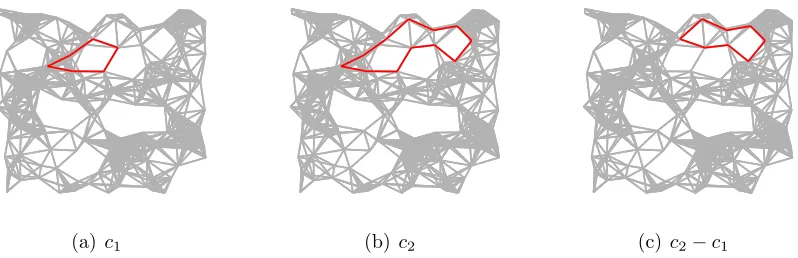
Note that homology by the above deﬁnition is well deﬁned because Img(∂k) ⊂ Ker(∂k−1). Two cyclesc1, c2 ∈ker(∂1) which are equivalent to each other in the quotient

space H1, i.e., c1 −c2 ∈Img(∂2) are said to be homologous to each other. As will be seen, these homology groups will be instrumental in uncovering the properties of our topological spaces. We will give a few important properties of these homology groups after the following basic deﬁnitions.

Deﬁnition Given two chain complexes C ={Ck, ∂k} and D={Dk, ∂k}, a chain map F# : C → D is a sequence of homomorphisms {Fk : Ck →Dk} such that the diagrams of the following type commute,

Ck F_k

−−−→ Dk ⏐

⏐ ∂_k

⏐ ⏐ ∂_k

Ck−1 F_k₋₁

−−−→ Dk−1 ,

i.e., ∂k◦Fk =Fk−1◦∂k.

The above deﬁnition states that the chain maps preserve the boundary operation. In other words, applying a chain map and followed by a boundary operator on the range chain complex is equivalent to ﬁrst applying a boundary operator followed by a chain map. Although we are using the same symbol ∂k to denote the boundary operators in

both chain complexes, which complex it belongs to should be clear from the context. We state the following theorem without proof [69]:

Theorem 2.4.1 A chain map f# : C → D induces homomorphisms f∗ : H∗(C) →

H_∗(D) on the corresponding homology groups.

(27)

Deﬁnition Let f, g:C →D be chain maps. We say that f is chain homotopic to g

if there are homomorphisms {φk} of graded abelian groups φk:Ck→Dk+1 such that

φk₋1◦∂k+∂k+1◦φk =f−g The operation of φ can be represented by the following diagram

Ck φ_k

−−−→ Dk+1 ⏐

⏐ ∂_k

⏐ ⏐ ∂_k₊₁

Ck−1 φ_k₋₁

−−−→ Dk

Chain Homotopy may also be viewed as analogous to homotopy of continuous maps, the diﬀerence being that one operates on chain maps while the other operates on topo-logical spaces. As we will see the subsequent section, we can form chain maps from a topological space at which point we will put all these concepts together. The following theorem is an important consequence of chain homotopies [69].

Theorem 2.4.2 Given two chain complexes C and D, if ∃ chain maps f : C →D and

g :D →C such that f◦g is chain homotopic to id and g◦f is chain homotopic to id, then the homology groups of the chain complexes Hk(C) and Hk(D) are isomorphic.

Finally we introduce the laplacian operators which, for our purposes, will be shown to greatly simplify the computational framework of homology groups.

Deﬁnition Given a chain complexC, thekth_{Laplacian operator}_L

k :Ck →Ckis deﬁned

as

Lk=∂k+1◦∂k∗+1+∂k∗◦∂k

where ∂_k∗ is the adjoint of∂k

When ﬁeld coeﬃcients are used, the chain spacesCkare vector spaces, and the

bound-ary operators have matrix representation for a given basis. The matrix representation for the adjoint operator ∂_k∗ is just the transpose of that of ∂k. It can be shown [55] that

(28)

2.5 Topological Analysis Revisited

Having deﬁned chain complexes, maps on chain complexes and the relation between ho-mologies of chain complexes, we close the loop by constructing a chain complex given a simplicial complex representing a Topological space.

We have seen in Section 2.3 that simplicial complexes are built from a collection of simplices by gluing together their faces. A complete deﬁnition of a simplicial complex is as follows,

Deﬁnition Given a set of verticesV, asimplicial complex K ={σi}is a collection of

simplices. Each simplex is determined by a set of vertices (v0, . . . , vk) inV, i.e.,σk is the

set of convex combinations of (v0, . . . , vk). The simplices have the following properties: • σi, σj ∈K ⇒σi∩σj ∈K

• All faces of σi are in K.

An important fact to note here, is that each simplex in a simplicial complex can be determined by a unique set of vertices.

2.5.1 Chain Complex from a Simplicial Complex

To construct a chain complex, we require a sequence of abelian groups{Ck}(chain spaces)

and a sequence of boundary operators{∂k} such that ∂2 = 0.

Building chain spaces

Given a simplicial complexK, we form an abelian group called a chain space{Ck(K)}by

considering all thek-simplices{σ_ik}as generators. Thus ifσk_i, σk_j ∈K, thena1σki+a2σkj ∈ Ck(K), a1, a1 ∈Z †.

(29)

Boundary Operators

The construction of the chain spaces Ck(K) is purely algebraic. We now relate the

algebraic structure in these chain spaces to the combinatorial structure in the simplicial complex K in two speciﬁc ways

1. For a given simplex σk, the additive inverse−σk will be related to the orientation of the simplices.

2. The boundary operator between the chain spaces Ck(K) and Ck−1(K) will be

re-lated to the relation between the simplices and their faces.

Note that we still have some additional algebraic structure left in the chain spaces, i.e., arbitrary coeﬃcients in Z, to which no meaning was assigned in the combinatorial structure. The additive inverse in terms of the orientation is given as:

if σk = (v0, . . . , vi, vi+1, . . . , vk) then −σk = (v0, . . . , vi+1, vi, . . . , vk) (2.2)

and, the simplices and their faces are linked using the boundary operators. Since {Ck(K)} is an abelian group, deﬁning the boundary operator ∂k : Ck(K) → Ck−1(K)

is equivalent to deﬁning it on each of its generators. Therefore, given a generator σk ₌

(v0, . . . , vk)∈Ck, we deﬁne the operation of a boundary operator as ∂k(v0, . . . , vk) =

i

−1i(v0, . . . , vi−1, vi+1, . . . , vk) (2.3)

Note that each summand is ak−1 simplex, hence the sum lies inCk−1(K). Veriﬁcation

of ∂2 = 0 is a straightforward but lengthy process. Therefore, we will show that it is in fact the case by considering an example. The operation of ∂1 ◦∂2 on a 2-simplex (v0, v1, v2) is

(30)

on topological spaces to homomorphisms and isomorphisms on algebraic spaces.

Theorem 2.5.1 [69] If X andY are topological spaces andKX, KY are simplicial

com-plexes representing these spaces, a map f :X →Y induces a chain map f# :C∗(KX)→

C_∗(KY) on their corresponding chain complexes. Further by theorem 2.4.1, f induces

a sequence of homomorphisms f_∗ : Hk(C∗(KX)) → Hk(C∗(KY)) on their corresponding

homology groups.

The theorem states that if there is a continuous mapping between two topological spaces, we can ﬁnd a corresponding homomorphism between their homology groups. In other words, any transformation in the topological spaces can be reﬂected as some transformation on the homology spaces. Again, notice the functorial property of assigning homology groups to topological spaces. An important extension of the above theorem follows.

Theorem 2.5.2 [69] Let X and Y be homotopy equivalent topological spaces, i.e., ∃ maps f :X →Y and g :Y →X such that f ◦g ≈id and g◦f ≈id. Then the induced chain maps are also chain homotopic to id, f# ◦g# ≈ id and g# ◦f# ≈ id. Further

by theorem 2.4.2, we have that the homology spaces Hk(C∗(KX)) and Hk(C∗(KY)) are

isomorphic.

The most important result to make note of is the implication of the above theorem which is enunciated as Homotopy equivalent spaces have isomorphic homology groups.

We noted in Section 2.2 referring to Figure 2.1, that homotopy equivalent spaces are similar in some sense (having a loop) even though they had diﬀerent geometrical proper-ties. The above theorem provides an alternative way of establishing such an equivalence by way of their homology groups (which are computable) being isomorphic.

(31)

2.5.2 Inferring Topological Properties from Homology groups

In order to understand what homology groups tell us about the topological space, we need to carefully look at the action of the boundary operators. Let us look at the null space (kernel) of ∂1. Consider a cycle c= e4 +e5 −e1 as shown in Figure 2.4 which is homeomorphic to a loop. The action of ∂1 is given as:

∂1(c) = ∂(e4+e5−e1)

= (v4−v1) + (v2−v4) + (v1−v2) = 0

This implies that the null space of ∂1 consists of all closed cycles (chains with zero boundaries). And as we saw in Equation 2.4, the boundaries of k + 1-simplices are closed cycles in Ck, and they belong to ker(∂k). This means that ker(∂1) also consists

of closed cycles which are boundaries of 2-simplices. But we know that 2-simplices are homeomorphic to disks. Therefore, if we remove all the cycles which are boundaries of 2-simplices, the cycles that remain are those circling a hole. From the deﬁnition of the homology group H1(C∗(KX) = ker(∂1)/Img(∂2), it is clear that H1 counts the number

of holes in our topological space. A similar explanation can be given to higher order homology groups; H2 counts the number of 3-dimensional voids and so on, albeit it is diﬃcult to visualize what the homology groups of order 3 and higher count. We now present an example to illustrate the basic mechanism of this procedure.

Example

We will now show how to compute the ﬁrst homology space for the simplicial complex shown in Figure 2.3, repeated in Figure 2.4. We start by constructing the chain spaces

C0, C1, and C2. Since there are no simplices of order greater than 2, all the chain spaces

Ck, k >2 are trivial. C0, C1,and C2 are vector spaces with the following basis sets:

C0 : {v1, v2, v3, v4}

C1 : {e1, e2, e3, e4, e5}

(32)

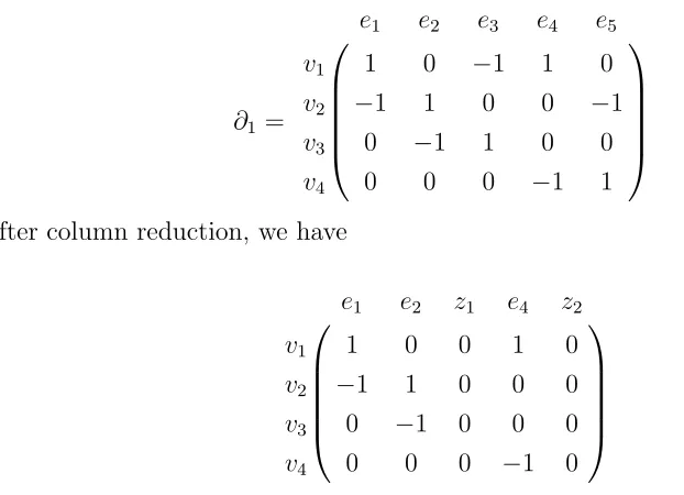
The matrix representation of the boundary operator ∂1 :C1 →C0 is given as:

∂1 =

⎛ ⎜ ⎜ ⎜ ⎜ ⎝

e1 e2 e3 e4 e5

v1 1 0 −1 1 0

v2 −1 1 0 0 −1

v3 0 −1 1 0 0

v4 0 0 0 −1 1

⎞ ⎟ ⎟ ⎟ ⎟ ⎠

after column reduction, we have

⎛ ⎜ ⎜ ⎜ ⎜ ⎝

e1 e2 z1 e4 z2

v1 1 0 0 1 0

v2 −1 1 0 0 0

v3 0 −1 0 0 0

v4 0 0 0 −1 0

⎞ ⎟ ⎟ ⎟ ⎟ ⎠

where z1 = e1 +e2 +e3, and z2 = e4 +e5 − e1. Therefore, ker(∂1) is spanned by {z1, z2}, and Img(∂2) is spanned by {e1 +e2 +e3}. The ﬁrst homology space is then

H1 =ker(∂1)/Img(∂2) ∼= span{e4+e5 −e1}. The ﬁrst homology has rank 1 which is equal to the number of holes in our topological space.

Let us look more closely at the quotient space H1. Consider the cycles c1 and c2 in Figure 2.4. It is clear from the ﬁgure, that they surround the same hole. The quotient spaceH1makes this similarity concrete. The diﬀerence of the cyclesc2−c2 =e1+e2+e3 ∈

(33)

v1

v2

v3 v4

e4

e5

e2

e3

−e1

σ1

c1 v1

v2

v3 v4

e4

e5

e2

e3

e1

σ1

c2

(34)

Chapter 3 Detection and Localization of

Topological Features

In this Chapter, we develop distributed algorithms to solve two seemingly unrelated prob-lems in sensor networks, 1) Coverage hole detection and localization and 2) Worm hole attack detection and localization. We do not assume any localization information of the nodes, nor any distances between the nodes.

(35)

3.1 Related Work

Distributed algorithms for analyzing topological properties in networks may be broadly classiﬁed into three categories: geometric, “topological”, and statistical methods. This categorization is based on the taxonomy presented in [70], and a good overview of algo-rithms in these areas is presented in [29]. We brieﬂy discuss some of these algoalgo-rithms to put our work in context.

Geometric Methods

In geometric methods, for example, the work in [29] computes an α-shape of the node positions in order to identify the outer and inner (coverage-hole) boundaries of a network. The authors assume that the distances between neighboring nodes is known. They use these distances to construct local coordinates and then go on to compute the α−shape. We discussα−shapes in more detail in Chapter 5 where we develop distributed algorithm to computeα−shape without the need for local coordinates. In this Chapter, we assume that the distances between neighboring nodes is unknown. Another example for geometric methods for the coverage problem is found in [26].

Statistical Methods

An example of a statistical approach to a coverage problem may be found in [62]. It relies on the idea that nodes close to network boundaries, have fewer incident edges in the network graph than internal nodes. The authors use statistical methods to derive suitable thresholds to separate edge nodes from internal nodes using the node degrees. In [63], boundary nodes are separated from internal nodes by using a centrality measure which counts the number of shortest paths that pass through a node. A higher centrality value occurs among internal nodes.

Topological Methods

(36)

observa-tion here is that each of these components has a discontinuity at the boundaries of the network. The algorithm is simple, and eﬀective given a high node density and uniform distribution of nodes. There is no simple way however, to provide theoretical guarantees on correctness of the algorithm, and quantify the required node density.

Algebraic topology, briefly introduced in Chapter 2, provides powerful tools to mean-ingfully define coverage holes only using the communication graph, and develop provably correct algorithms. Application of homology spaces to the coverage problem was first introduced in [19]. Given a set of “fence” edges, the work in [19] provides a necessary and sufficient condition to verify the coverage inside the fence, and recent work in [20] provides a distributed algorithm to perform this verification. When coverage cannot be guaranteed, [33] gives a criterion using persistent homology to guarantee the existence of holes.

In our context, in addition to detecting the presence of holes, we need an distributive algorithm to localize the holes. The work in [76] describes a methodology to compute localized generators given a cover. Given a subdivision of the entire space into subsets, they find an appropriate cover, and check for existing homology classes. To the best of our knowledge, [66] is the first attempt at distributively localizing holes, by formulat-ing the localization as an optimization problem. Given a non-contractible cycle c, [66] looks for a cycle which minimizes the l1 norm in the set of homologous cycles [c]. They show, that under certain conditions, minimizing thel1 norm produces the same result as minimizing the l0 norm, where the latter case localizes the holes. For general simplicial complexes, the problem of minimizing the l1-norm of a cycle up to a constant factor is NP-hard [12]. Hence, such optimization algorithms necessarily rely on iterative algo-rithms whose convergence rate is usually slow, and difficult to analyze. In this Chapter, by forgoing the requirement of computing explicit cycles, and exploiting the fact that the nodes are deployed on a plane, we show that a distributive localization of coverage holes may be achieved very efficiently.

(37)

authenticate themselves as legitimate nodes to the network. When initiating a wormhole attack, an attacker overhears packets in one part of the network, tunnels them through the wormhole link (external to the network) to another part of the network. This eﬀec-tively generates a false scenario of the presence of the original sender in the neighborhood of the remote location.

Many routing algorithms depend on the nodes’ ability to accurately discover their neighboring nodes. The nodes ordinarily perform a broadcasting beacon (including ID, and other information) to their neighbors. If the neighbor discovery beacons are tun-neled through wormholes, the good nodes will get false information about their route. Although ﬁnding faulty routes is in itself a problem, worm holes can cause further crit-ical security threats using these faulty routes. The resulting eﬀect of wormholes on the routing, is to include a worm hole link in most of the computed routes. This in turn, gives an attacker complete control of transmitting great amounts of data, which may be selectively or completely dropped. Impacts of a wormhole on a route discovery procedure in a sensor network, have been studied at length in [37, 47].

(38)

3.2 Formalization of topological network failures

3.2.1 Coverage Problem

We consider the scenario where N sensor nodes are randomly deployed in a region of interest. We denote the collection of all the nodes as the set V ={vi}. Each node vi can

communicate with all the nodes within a circular neighborhood Ri

s of radius rs, and we

denote these nodes as the setNi, the neighbors ofvi. A communication graphG= (V, E)

is thus formed as the collection of the set V together with the set of edgesE ={(vi, vj)}

where (vi, vj) ∈E, if and only if vi, vj can communicate with each other. The coverage area of a sensor at each node is assumed to be a circular neighborhood Ri

c of radius rc

centered at nodevi. Denote the union∪iRicof coverage ares asRc, the total coverage area.

Deﬁne the embedded 1-skeleton of the communication graph as a collection of points and line segments in the plane. The location of the points is given by the location of nodes, and the line segments are the lines between those points, whose length is less than the communication radius. Now, the boundary ∂() of this embedded 1-skeleton is the union of line segments which encloses all the nodes. The region of interestis the region enclosed by this 1-skeleton boundary. The objective is to identify if the following relation holds

⊆Rc (3.1)

This highlights our interest in being completely covered by the coverage areas of the sensors. The outermost boundary of a sensor network is to some extent controlled by the deployer, and there are algorithms which can detect this boundary [71]. As Equation (3.1) suggests, we are therefore mainly interested in the coverage of the region “inside” the network. Furthermore, if the relation (3.1) does not hold, our goal is to ﬁnd the nodes on the shortest path surrounding the components in ∂() of the uncovered region.

(39)

any sensor, we seek the smallest cycle in the network surrounding this coverage hole.

We make the following assumptions about the technological resources and constraints:

1. We can adjust the communication radius. Note that this may be easily achieved by adjusting the power to the antenna

2. The nodes have no coordinate information.

3. There is no direction information, i.e., the nodes are unaware of the relative orien-tation of their neighbors.

4. The nodes are not necessarily uniformly distributed in a given region of interest.

3.2.2 Worm Hole Problem

A worm-hole attack is typically launched by two colluding nodes at positions p1 and

p2 inside a network. Denote the neighborhood regions around these points by N1 and

N2. The two attacking nodes may receive all the packets transmitted from within their

respective neighborhoods, and relay them to the other. Denote by V1 and V2 the sets of vertices (sensor nodes) which lie in N1 and N2 respectively. The result of a worm-hole attack will be to produce a complete bi-partite graph with V1 and V2 as the two classes of vertices. The problem of localizing a worm hole attack, hence reduces to identifying the sets V1 and V2. In addition to all the above assumptions pertaining to the coverage problem, we will also assume the following:

1. The positionsp1andp2are suﬃciently far apart from each other inside the network, such that N1∩N2 =φ. This is a suﬃcient condition for us to detect a worm hole attack.

(40)

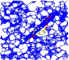
Figure 3.13 shows an example of a worm hole attack. In this case, X and Y are the positions p1 and p2 and the neighborhoods A and B are N1 and N2 according to our deﬁnition.

3.3 Preliminaries

3.3.1 Coverage area and the ˇ

Cech complex

As discussed in Section 2.3, topological spaces can be represented using simplicial com-plexes. The simplicial complex which can accurately† represent the coverage area is the

ˇ

Cech complex [68].

Note that the coverage area is a union of convex sets. Given a collection of sets

Rc =

iRic , the ˇCech complex ofRc,KN(Rc), is the abstract simplicial complex whose k-simplices correspond to nonempty intersections of k+ 1 distinct elements of Rc. An

edge in KN(Rc) exists between two vertices if and only if the corresponding elements

of Rc intersect. Higher dimensional simplices are regulated by mutual intersections of

collections of elements of Rc. Among the many uses of nerves in topology, the following

classical result is perhaps of greater importance in applications:

Theorem 3.3.1 (The ˇCech Theorem): The ˇCech complex of a collection of convex sets

is topologically equivalent to the union of the sets [68].

The implication of this theorem is that KN(Rc) effectively captures the topology of Rc, and the first homology (introduced in 2.4)H1(KN), is isomorphic to the first

homol-ogy H1(Rc) of the coverage area. The computation of the nerve complex unfortunately requires localization information, and is very diﬃcult even when we have it. We therefore rely on an approximate representation called the Vietoris-Rips (or Rips in short) com-plex, denoted by Kp(Rc) which may be obtained only from the communication graph.

For extracting the Rips complex, we simply say that each k clique in the communica-tion graph is a k −1 simplex in the Rips complex. We choose a communication radius

rs = 2rc, where rc is the coverage radius.

(41)

3.3.2 Approximation by a Rips complex

The Rips complex Krs

p obtained with choice of communication radius rs= 2rc is a good

approximation to KN in the following sense. Owing to their construction, both KN and K2rc

p share the same set of 1-simplices. Also, as Kp2rc is the maximal simplicial complex

with a given set of 1-simplices, KN ⊂ Kp2rc. In what follows, we use the inclusion map i:KN →K2rc

p and the induced homomorphism i∗ :H1(KN)→H1(Kp2rc).

1. If there exists a non-trivial homology class [cp]= 0 inH1(Kp2rc), then there exists a

corresponding non-trivial homology class [cN]= 0 inH1(KN), such thati∗([cN]) =

[cp]. This implies that we do not create any false alarms.

2. When there is a non-trivial homology class [cN]= 0 inH1(KN), such thati∗([cN]) =

0, then cN can be expressed as a boundary of 2-simplices in Kp2rc. This means

that when a hole is missed, it is conﬁned to a region formed by a triangle in the communication graph.

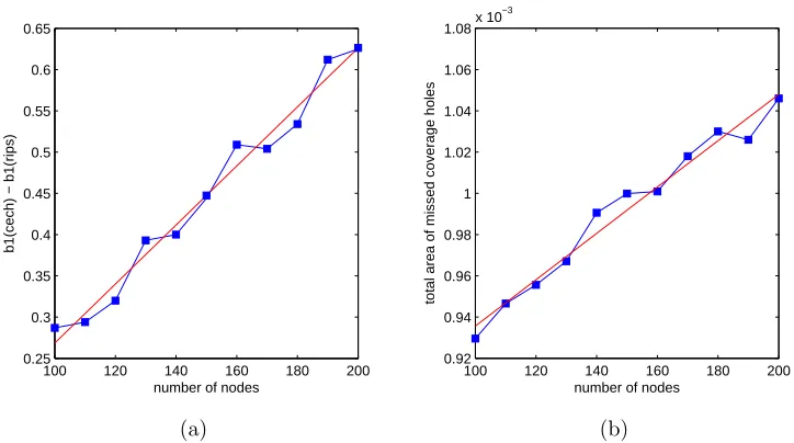
3. The diﬀerence in the betti numbers ofK2r_c

p andKN grows asO(n) as proven in [44],

and demonstrated by a simulation in Figure 3.1(a). This means that on average, the number of missed holes will be proportional to the size of the network, which is important from the perspective of scalability.

4. The total area of the missed holes is a very small proportion compared to the total area of deployment, as shown in Figure 3.1(b).

The ﬁrst two points immediately follow from the fact that both KN and Kp2rc share

the same 1-skeleton, and that KN ⊂ Kp2rc. The results shown in Figures 3.1(a) and

3.1(b) were averaged over 1000 realizations of random geometric graphs. To compute the total coverage hole area missed, we first find all the triangles for which the circumcenter is not covered, and compute the uncovered area in each. Note that we only check for a necessary (but not sufficient) condition, and therefore, Figure 3.1(b) shows the upper bound of the missed area. Figure 3.2 shows a case when a coverage hole, which is enclosed by a triangle in the communication graph, is missed (“filled”) by the Rips complexK2rc

(42)

100 120 140 160 180 200 0.25 0.3 0.35 0.4 0.45 0.5 0.55 0.6 0.65

number of nodes

b1(cech) − b1(rips)

(a)

100 120 140 160 180 200 0.92 0.94 0.96 0.98 1 1.02 1.04 1.06 1.08x 10

−3

number of nodes

total area of missed coverage holes

(b)

Figure 3.1: (a)shows the average of the diﬀerence between the ﬁrst Betti numbers ofK2rc

p

and KN. A formal proof of this relationship can be found in [44]. (b) shows the upper

bound for the mean area of the coverage holes missed. The regression line is shown in red in both the ﬁgures.

Figure 3.2: A triangle in the communication graph, considered “ﬁlled-in” in, may contain a coverage hole.

3.3.3 Distributed Computation

(43)

information be avoided if at all possible. The algorithm we propose here, satisﬁes all these basic requirements.

An interesting class of distributed algorithms is that of gossip algorithms, where nodes process the data by passing messages amongst their neighbors. One particular gossip algorithm we exploit extensively, is the distributed computation of eigenvalues of a symmetric matrix in a network [45], using the orthogonal (or power) iteration method. In particular, as described in Section 3.4.2, we wish to compute the spectral radius of the ﬁrst order laplacianL1 of the Rips complex Kp2rc. We can extract the Rips complex from

the communication graph, distributively computeL1 and its spectral radius as described in [56]. We also develop some simple gossip algorithms and prove their eﬃcacy in the following sections as and when required.

3.4 Coverage Hole Localization

3.4.1 Algorithm Overview

As discussed in Section 2.4, the presence of a hole in the coverage space can be detected by the non-triviality of the ﬁrst homology space H1(Rc), which might be approximated closely with H1(Kp2rc) as justiﬁed in Section 3.3.2. IfH1(Kp) is non-trivial, we partition

the network in two parts in such a way that the process does not destroy any holes. We then check for the presence of holes in both parts. By repeating the above process, we converge on to the location of the holes.

3.4.2 Hole Detection

(44)

Theorem 3.4.1 LetL1 be a symmetric non-negative deﬁnite matrix with spectrumσ(L1),

and spectral radius ρ(L1). Then, L1 is rank deﬁcient if ρ(ρ(L1)I−L1) =ρ(L1)

Proof Let x be an eigenvector corresponding to the eigenvalue λ ∈ σ(L1). Then (ρ(L1)I−L1)x= (ρ(L1)−λ)x. ⇒xis also an eigenvector of (ρ(L1)I−L1) and its eigen-value isρ(L1)−λ. Furthermore,L1 is non-negative deﬁnite⇒ λ≥0 ⇒ρ(ρ(L1)I−L1)≤

ρ(L1) if L1 is of full rank, thenλ >0 ⇒ρ(ρ(L1)I −L1)< ρ(L1).

The spectral radius of L1 can be computed using the power iteration method by searching for the largest eigenvalue which can be distributively carried out over the net-work [45]. The convergence of the power iteration method (for eigenvector) is slow when the diﬀerence between the largest and second largest eigenvalue is small, while the eigen-value itself quickly converges to the true eigen-value.

Each iteration in the power iteration method includes multiplyingL1 by a vector from the previous iteration, and normalizing the resulting vector. The sum of the squared ele-ments of the vector (for normalization) can also be distributively computed in the network by a gossip algorithm whose convergence time is of order Θ (nlog(n)) [7, 8].

The mixing time of natural random walks on geometric random graphs is of the order Θ(r−2logn) [8]. The natural random walk is one where the transition from a node to any of its neighbors is equally likely. The algorithm for computing the sum over the network nodes, is based on such a random walk. Each step of the walk corresponds to a node transmitting a message to one of its neighbors, and the mixing time corresponds to the convergence time of the algorithm. Therefore, the message passing complexity is equivalent to the time complexity. In our work, we set the communication radius to be of the order r2 = k_n, where k is a constant, so as to maintain a constant mean node degree.

3.4.3 Hole Localization

(45)

equivalence class. The definition of shortest closed path is accurate only for convex holes in the coverage area. For a given set of points in a plane, it is a non-trivial problem to define the shape of these points, and hence the boundary of hole. The definition of shortest closed path to localize the coverage hole is still appropriate in general as it is a good approximation.

A very direct approach was proposed in [66], where the authors formulate the local-ization as an optimlocal-ization problem to seek the sparsest chain in the H1 space. Such an approach is eﬀective, but at a cost of a very slow convergence, and involves all the nodes in the network until the iterative algorithm converges. In contrast, in our algorithm, all the nodes which belong exclusively to a subset with trivial homology no longer participate.

When we detect a hole in the network, as in Section 3.4.2, we partition the network into two subnetworks and detect the presence of the holes in each. We make sure that such a division does not destroy any holes, a condition necessary for this strategy to successfully localize the coverage holes. Furthermore, we want to divide the network in such a way that resulting parts (or partitions) are approximately of the same size. In order to perform such a division, we ﬁnd a pair of nodes which are farthest from each other in the network, and divide the network along the nodes which are equi-distant (±1 hops) in hop length from this pair. The nodes in such a pair are denoted as diameter nodes and the node equi-distant from them as boundary nodes.

Finding Diameter Nodes

Formally, the diameter nodes are deﬁned as

(¯u,v¯) = arg max

(v_i,v_j) d(vi, vj), (3.2)

where d(vi, vj) is the shortest path between nodes vi and vj (in terms of hop count).

Such a pair will generally not be unique, and “ties” between nodes are broken by a simple protocol which chooses the pair that has the node with the smallest ID.

(46)

Cdia by assigning a scalar ﬁeld f(vi) equal to the farthest distance for each node x

in the current partition, and to ultimately select the nodes with the maximum f; we subsequently proceed to break the “ties” using the afore mentioned criterion,

f(vi) = max

v_j d(vi, vj), Cdia={v|f(v) = max

v_j f(vj)}. (3.3)

To compute f onG, we use a simpliﬁed version of the Dijkstra’s algorithm. The simpli-ﬁcation is a result of the following, a)we do not need the shortest paths but rather just the distances and b)Instead of shortest distance from a node vi to all other nodes, we

require max of distances.

A summary of the algorithm for computing f is given in Table 3.1. In what follows, we provide an intuition into the mechanics of the algorithm followed by a mathematical justiﬁcation.

It immediately follows from Equation (3.3) that, in order to compute f(x), it is suﬃ-cient for each nodevi to have the knowledge ofd(vi, vj) for allvj inG. Sincef(vi) has to

be computed for allvi, the preceding statement may equivalently be stated as follows; for

each vi, it is suﬃcient for all vj (all other nodes) to know d(vi, vj). We accomplish this

by broadcasting nodevi’s id in the network, and for each nodevj,d(vi, vj) is equal to the

number of hops taken by the ﬁrst message arriving atvj. Note that, in order forvi’s id to

(47)

Denote by A= {aij}, the adjacency matrix for G, then An =anij, n >0 where anij is

the number of paths of length n from i toj [34]. For simplicity, we assume that i is the ID given to node vi. Now, the shortest distance from vi to vj, i=j is given by

d(vi, vj) = arg min n>0 a

n

ij >0, i=j (3.4)

The matrix An _{can be distributively represented in the network where node} _v i

com-putes and stores the ith _{row. This can be iteratively computed as} _An+1 ₌ _A·_An_{, and} an_ij+1 at node vi is obtained as anij+1 =

v_k∈N(v_i)a n

kj. This computation is enabled by all

the nodes broadcasting their row to their neighbors. Ifmis the smallest integer such that

am_ij >0, this implies there is no path fromvitovjof length smaller thanm. Therefore, the node i “discovers” node j at iteration m, and at this instant, is a ”new” node. Further, if k∈N(i), this also implies am_kj+1 >0, and the values ofan

kj for n > m+ 1 are irrelevant

from the perspective of computing d(vk, vj). We therefore refrain from broadcasting amij

for n > m time intervals. In other words, each node broadcasts the information about a new node it discovers only once. Note that in so doing, we do not actually compute

An _{at the} _nth _{iteration, but an estimate ˆ}_An _{with the property that the smallest integer} m for which ˆam_ij > 0 is that for am_ij > 0. The table used, acts as a reference to avoid transmitting duplicate information to its neighbors. Here, it appears that the memory required at each node will be equal to the number of nodes in the partition, as all the nodes will eventually be discovered. We maintain that it suﬃces to store a node in the table for only two iterations.

Theorem 3.4.2 A node vi storing the information about the nodevj for two iterations,

guarantees no duplicate information is broadcasted.

The proof of the theorem is given in appendix A.0.1. If nmax is the largest distance

for which a node vi discovers a new node, then we set f(vi) =nmax.

(48)

Table 3.1: Finding Diameter Nodes (left) and Boundary Nodes (right)

At each Node i in the segment

\\ Computing f

\\ Initialization: Discover itself add vi to table and broadcast to N(i)

\\ run time at iteration n:

\\check for new nodes discovered

if found new nodes

broadcast new nodes to N(i) add new nodes to table clear values of n-2 iteration

else

f(vi) =n

stop.

At each Node i in VX

\\Initialization

if vi is a diameter node

broadcast i toN(i). stop. (i will serve as the segment ID)

else

wait until reception

if received two distinct IDs

broadcast the lowest received ID toN(i).

vi = boundary node. wait one time interval

if received two distinct IDs overall

vi = boundary node. stop.

broadcasts this discovered value to all its neighbors. Similarly, the diameter nodes are obtained from the candidate nodes by consensus for a minimum of node IDs.

Finding Boundary Nodes

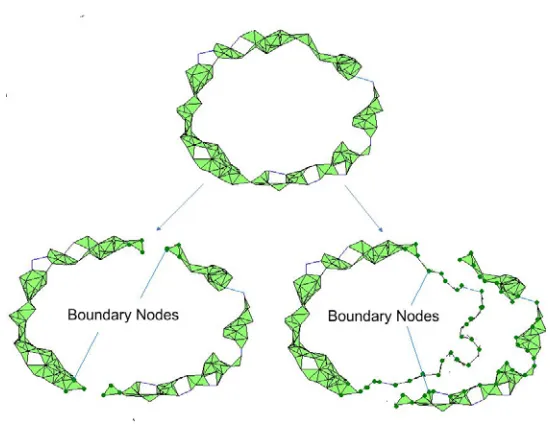
As the physical positions of the nodes do not change, we form a virtual segmenta-tion by ﬁnding boundary nodes B = {bi} within a partition which stop messages from

passing through. This eﬀectively separates a given partition into two parts with non-intercommunicating nodes. For a set B to behave like a boundary†, it has to satisfy certain properties:

Deﬁnition Let X = (VX, EX) ⊆ G be a connected sub-graph. The set of nodes B is

said to be a boundary in X, if and only if ∃ two disjoint sets VX1, VX2 ⊂ VX such that

there is a node bi ∈B in any path (vi, . . . , vj), wherevi ∈X1 and vj ∈X2. Furthermore,

VX1∪VX2∪B =VX.

†_{This deﬁnition of a boundary should not be confused with the conventional notion, confounded with}

Topology and Geometry of Sensor Networks: A Distributed Computing Approach.

ABSTRACT

DEDICATION

BIOGRAPHY

ACKNOWLEDGEMENTS

Table of Contents

LIST OF TABLES

LIST OF FIGURES

Chapter 1

Introduction

Chapter 2

Algebraic Topology

2.1

Topology

2.2

Topological Analysis

2.3

Representation of Topological Spaces

2.3.1

Simplicial Complexes

2.4

Homological Algebra

2.5

Topological Analysis Revisited

2.5.1

Chain Complex from a Simplicial Complex

2.5.2

Inferring Topological Properties from Homology groups

Chapter 3

Detection and Localization of

Topological Features

3.1

Related Work

3.2

Formalization of topological network failures

3.2.1

Coverage Problem

3.2.2

Worm Hole Problem

3.3

Preliminaries

3.3.1

Coverage area and the ˇ

Cech complex

3.3.2

Approximation by a Rips complex

3.3.3

Distributed Computation

3.4

Coverage Hole Localization

3.4.1

Algorithm Overview

3.4.2

Hole Detection

3.4.3

Hole Localization