Theoretical Analysis of SDA/SAA and CASTS Algorithms for Service Differentiation.

ABSTRACT

ZHANG, HUIJUN. Theoretical Analysis of SDA/SAA and CASTS Algorithms for Service Differentiation. (Under the direction of Dr. Yannis Viniotis.)

© Copyright 2012 by Huijun Zhang

Theoretical Analysis of SDA/SAA and CASTS Algorithms for Service Differentiation

by Huijun Zhang

A thesis submitted to the Graduate Faculty of North Carolina State University

in partial fulfillment of the requirements for the Degree of

Master of Science

Computer Engineering

Raleigh, North Carolina

2012

APPROVED BY:

Dr. George N. Rouskas Dr. Michael Devetsikiotis

DEDICATION

BIOGRAPHY

Huijun Zhang was born on September 28th, 1988 in Yangquan, Shanxi, China. She graduated from Zhejiang University in June 2010, with a Bachelor of Engineering degree in Electronics and Communication. Her undergraduate thesis was titled “Design of Polarization System”.

Huijun has been working towards her Master of Science degree in Computer Engineering at North Carolina State University since August 2010. She has decided to change major to Networking. She is currently working on her thesis under the guidance of Dr. Yannis Viniotis. Her research interest is Service Oriented Networking.

ACKNOWLEDGEMENTS

I would like to express utmost gratitude to my advisor Dr. Viniotis for giving me the valuable opportunity to work on my Master’s thesis under his extremely patient help. His knowledge, precise judgement, and solemn attitude gave me a great academic and life guidance. I am also grateful to him for providing me an opportunity to be a TA at NCSU.

My gratitude to Dr. George Rouskas and Dr. Michael Devetsikiotis for serving on my the-sis committee, and help me with my thethe-sis defence. Special thanks to Mursalin Habib and Keerthana Boloor for their help on understanding their work which formed the basis for my thesis.

TABLE OF CONTENTS

List of Figures . . . vii

Chapter 1 Introduction and Motivation . . . 1

1.1 Web Services and Service Oriented Architecture . . . 1

1.1.1 What is a Service? . . . 1

1.1.2 What is a Web Service? . . . 1

1.1.3 Architectures and Implementations of Web Services . . . 2

1.1.4 SOA . . . 2

1.2 Prior Work Survey . . . 3

1.2.1 Service Differentiation . . . 3

1.2.2 Prior Approaches . . . 4

1.3 Motivation and Contribution . . . 4

1.4 Outline of the Thesis . . . 5

Chapter 2 Overall System Architecture . . . 6

2.1 Service Domains . . . 6

2.2 Gateway and WRR Scheduler . . . 7

2.3 Appliances . . . 7

2.4 Statistic Collection and SDA/SAA Block . . . 8

2.5 Service Tier . . . 8

Chapter 3 Proof of Convergence of the SDA/SAA Algorithm. . . 9

3.1 SDA/SAA Algorithm Description . . . 9

3.1.1 Terminology . . . 9

3.1.2 Algorithm Description . . . 10

3.1.3 Assumptions and Notations for Proof . . . 12

3.2 Preliminary Results . . . 13

3.3 Statistical properties of the utilization sequence . . . 16

3.4 The Main Result . . . 21

3.5 Extended Results . . . 22

Chapter 4 Conclusion and Future Work . . . 23

4.1 Summary and Conclusion . . . 23

4.2 Future Work . . . 23

References. . . 25

Appendix . . . 26

Appendix A CASTS Algorithm Proof . . . 27

A.1 Problem Definition . . . 27

A.2 Description of CASTS Algorithm and Manual Static Algorithm . . . 27

A.2.1 CASTS Algorithm Introduction . . . 27

A.2.3 CASTS Algorithm . . . 29

A.2.4 Manual Static Allocation . . . 30

A.3 Proof . . . 30

A.3.1 CaseB = 1, K= 1 . . . 30

A.3.2 CaseB 6= 1, K= 1 . . . 30

A.3.3 CaseB = 1, K6= 1 . . . 31

LIST OF FIGURES

Figure 2.1 The abstract system model . . . 7

Chapter 1

Introduction and Motivation

1.1

Web Services and Service Oriented Architecture

1.1.1 What is a Service?

Service can be defined as a component capable of performing a task. In the information and technology fields, service is a mechanism by which a consumer’s need or want is satis-fied according to a negotiated contract (implied or explicit) which includes service agreement, function offered and so on [10]. It includes technical support, computer networking, systems administration, and other IT services. Common Internet services, such as web hosting, e-mail, and social networking websites also fall under the scope of technology services.

Information and technology services may also include services not directly related to infor-mation technology, such as telephone and cable TV services. Other industries, such as digital photography, graphic design, and video production may also be considered technology services, since they involve modern technology.

1.1.2 What is a Web Service?

A Web service is a method of communication between two electronic devices over the web (internet). The World Wide Web Consortium (W3C) defines a “Web service” as “a software system designed to support interoperable machine-to-machine interaction over a network”. It has an interface described in a machine-processable format (specifically Web Services Descrip-tion Language, known by the acronym WSDL). Other systems interact with the Web service in a manner prescribed by its description using SOAP messages, typically conveyed using HTTP with an XML serialization in conjunction with other Web-related standards. [5]

and still can express complex messages and functions. The HTTP protocol is the most widely used Internet protocol. The main Web services platform elements include: SOAP (Simple Object Access Protocol); UDDI (Universal Description, Discovery and Integration); and, WSDL (Web Services Description Language).

Why use web services in the first place? Firstly, for their interoperability advantages: when all major platforms could access the Web using Web browsers, different platforms could interact. For these platforms to work together, Web-based applications were developed. Web-based ap-plications are simply apap-plications that run on the web. These are built around the Web browser standards and can be used by any browser on any platform. Secondly, Web services take web applications to next level: by using Web services, an application can publish its function or message to the rest of the world. Web services use XML to code and to decode data, and SOAP to transport it (using open protocols). With Web services, for example, an accounting depart-ment’s billing system deployed on a Win2k server platform can connect with an IT supplier’s UNIX server. [11]

1.1.3 Architectures and Implementations of Web Services

The three most widely deployed architectures and implementations of Web Services are RPC, REST and SOA.

Remote procedure call (RPC): RPC Web services present a distributed function (or method) call interface that is familiar to many developers. Typically, the basic unit of RPC Web services is the WSDL operation.

Representation state transfer (REST): REST attempts to describe architectures that use HTTP or similar protocols by constraining the interface to a set of well-known, standard op-erations (like GET, POST, PUT, DELETE for HTTP). Here, the focus is on interacting with stateless resources, rather than messages or operations. Clean URLs are tightly associated with the REST concept.

Service-oriented architecture (SOA): Web services can also be used to implement an archi-tecture according to SOA concepts, where the basic unit of communication is a message, rather than an operation. This is often referred to as “message-oriented” services. We focus on this architecture next.

1.1.4 SOA

the phases of system development and integration.

The following guiding principles define the ground rules for development, maintenance, and usage of SOA [2]:

a. reuse, granularity, modularity, composability, componentization and interoperability. b. standards-compliance (both common and industry-specific).

c. services identification and categorization, provisioning and delivery, and monitoring and tracking.

There are three types of architectures: application, service, component. Application Archi-tecture is the business-facing solution which consumes services from one or more providers and integrates them into the business processes. Service Architecture provides a bridge between the implementations and the consuming applications, creating a logical view of sets of services which are available for use, invoked by a common interface and management architecture. Component Architecture describes the various environments supporting the implemented applications, the business objects and their implementations.

SOA is implemented for a variety of reasons. Security: the Web Services Security specifi-cation addresses message security. This specifispecifi-cation focuses on credential exchange, message integrity, and message confidentiality. Reliability: in a typical SOA environment, several doc-uments are exchanged between service consumers and service providers. Delivery of messages with characteristics like once-and-only-once delivery, at-most-once delivery, duplicate message elimination, guaranteed message delivery, and acknowledgement become important in mission-critical systems using service architecture. Management: as the number of services and business processes exposed as services grow in the enterprise, a management infrastructure that lets the system administrators manage the services running in a heterogeneous environment becomes important. [7]

1.2

Prior Work Survey

1.2.1 Service Differentiation

allocating resources for execution of individual Web service requests [1].

1.2.2 Prior Approaches

We can classify prior work in the Service Differentiation space (and more specifically the CPU resource allocation space) under three generic approaches. The classification makes use of the system architecture model and terminology we introduce in the next chapter.

Approach 1: “manipulate the service process”. Under this approach, client traffic enters the appliance as is and CPU scheduling (as discussed, for example, in [9]) is used as the control mechanism to differentiate client traffic. It requires per domain buffering (and typically used in the server tier of the model we will discuss in the next chapter).

Approach 2: “manipulate the arrival process”. Under this approach, we control the rate at which client traffic enters the appliance. In a stable system, this effectively controls the output rate and hence the service the client traffic receives. We refer to this arrival control as activation/deactivation of traffic at the gateway. If, for example, more CPU resource is required to achieve the goal, client traffic rate gets increased. Thus we control the allocation of resources or performance class indirectly, as resource utilization or performance depends on arrival rate of that client. [6]

Approach 3: distinguish congestive and non-congestive queue. It is simple but powerful tool implemented in gateway since non-congestive flows do not cause significant delays and hence should not suffer from delays. Non Congestive Queuing (NCQ) is used as a specific scheduling discipline. It shows that (i) non - congestive data gets a much better service from the network, (ii) congestive data suffers no extra delays; instead, both fairness and efficiency are occasionally improved due to lower contention. Having more flows finishing early may lead to better resource sharing and more user satisfies. It is particularly beneficial for applications that utilize small rates and short packets. [8]

1.3

Motivation and Contribution

The work in [6] provided the first known methodology to provide service differentiation and make efficient use of appliance resources. The (SDA/SAA) algorithm proposed in [6] was shown to have good implementation advantages, but was evaluated via simulations only. In this thesis our motivation was to strengthen the commercial appeal of this algorithm by proving analytically that it possesses the capability of satisfying service guarantees.

1.4

Outline of the Thesis

The thesis is organized as follows. In Chapter 2, we introduce the system architectural model used for implementing activation/deactivation of service domains at the gateway. We explain in sufficient detail the main components of the model, so that the mathematical model can be later formulated. In Chapter 3, we introduce the SDA/SAA Algorithm and provide the proof that it can achieve and desired CPU utilization. We outline the assumptions necessary for this proof. We conclude in Chapter 4 with a summary and a suggestion for future work.

Chapter 2

Overall System Architecture

In this chapter, we present a system model that abstracts the operation of the real systems. The model can be used to formally describe the SDA/SAA activation/deactivation algorithm and define the quantities of interest in stating and proving our main result.

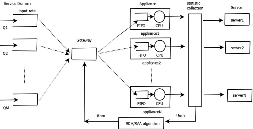
The model was first used in [6] and is shown in Figure 2.1. It captures the operations of modern-day multi-tiered data centers or back-end offices in which large scale applications run on one or multiple servers (i.e., the service tier). These applications use the services of specialized “appliances” (also known as application controllers) which are typically deployed in a separate tier that resides in front of the service tier as Figure 2.1 suggests.

A typical request is served first in the appliance CPU and then the server CPU. Traffic into an appliance comes from the gateway device. This device collects traffic from users who may be dispersed all over the world.

We describe next some of the important elements of this architecture.

2.1

Service Domains

Service requests to be served in the system arrive at the gateway from clients, over a trans-port network. Different types of service requests are grouped intoService Domains. In a certain service domain, there are multiple service requests waiting in a first come first serve queue. We assume that there areM such service domains.

Figure 2.1: The abstract system model

2.2

Gateway and WRR Scheduler

The gateway is the first entry point of the system, where service requests from customers arrive via a transport network. Requests are placed in queues organized per service domain. Traffic from these queues is forwarded to an appliance for processing at the appliance CPU. The selection of the next packet to be forwarded to an appliance is governed by a Weighted Round-Robin (WRR) scheduler. Each service domain is assigned a weight.

The weights are not static, as is usually the case with WRR scheduler deployments. They are rather determined using feedback from the appliances. This feedback is collected by the statistics collection box as shown in Figure 2.1. As we will explain in more detail in the next chapter, this feedback contains information about CPU utilization in the appliances. The box labelled SDA/SAA algorithm processes this feedback and directs the gateway to change the WRR weights.

2.3

Appliances

manner.

There are alternative architectural ways to deploy appliances, like using series connection between each other instead of parallel connection, which will reduce the cost of calculation. However, this parallel connection model can process multiple requests at the same time, and reduce average waiting time to a great extent.

2.4

Statistic Collection and SDA/SAA Block

This block (alternatively called the “provisioning agent”) is responsible for collecting statis-tics from the appliances and calculating the WRR weights for the gateway. An increase of one unit in the weight of a service domain has been known as an “activation of an instance” of this domain; similarly, a decrease of one unit in the weight of a service domain has been known as a “deactivation of an instance” of this domain. The block is a logical entity. It may be implemented in one or more appliances or as a stand-alone or distributed application.

2.5

Service Tier

Chapter 3

Proof of Convergence of the

SDA/SAA Algorithm

In this chapter, we provide a mathematical proof that the SDA/SAA algorithm will achieve the target CPU utilizations. Our main result is Theorem 1 in Section 3.4. The result states that the sequence of utilizations achieved by the SDA/SAA algorithm will converge almost surely to the specified target CPU utilizations. In Section 3.1, we provide a summary description of the algorithm and how it is implemented in the system model described in Chapter 2. Furthermore, we state some assumptions that are necessary for the proof. In Section 3.2, we state and prove two preliminary lemmas regarding WRR scheduler properties. In Section 3.3, we study the statistical properties of the utilization sequence; they form the foundation of the convergence proof, which we present in Section 3.4. We outline and prove some extensions in the last section of this chapter.

3.1

SDA/SAA Algorithm Description

In order to describe the algorithm formally, we need to introduce some terminology first. The terminology is borrowed from [6].

3.1.1 Terminology

Decision Instant (Tk)is thekthdecision instant at which PA activates/deactivates service

domain instances based on the algorithm outcome. At Tk, all the measurements collected in

the time interval (Tk−1, Tk] are evaluated; activation and deactivation of service domains are

enforced. In our proofs,Tk is assumed to form a periodic sequence, for simplicity.

Target CPU percentile (Pm)is the desired percentage of CPU resources to be allocated

to themth service domain.

Achieved CPU percentile (Xm(Tk)) is the percentage of the cluster CPU resources

obtained by themth service domain until timeTk.

Down and Up Tolerances DTm andU Tm: in order to avoid unnecessary oscillations and

overhead, when the Achieved CPU percentile is “close enough” to the Target CPU percentile, i.e., when

Pm−DTm < Xm(Tk)< Pm+U Tm, (3.1)

the service domain is excluded from activation/deactivation.

Utilization Matrix (Unm) is the achieved resource utilization (e.g., total CPU time used)

by the mth service domain in the nth appliance, in the time interval (Tk−1, Tk].

Instantiation Matrix (Bnm) is the number of instances of the mth service domain that

should be activated in the nth appliance during the time interval (Tk−1, Tk]. This is the main

decision variable that the PA computes.

N is the total Number of Appliancesin the cluster.

M is theNumber of Service Domains supported by the system.

Groups A and D denote the ranking of service domains. When service domainm is not achieving its Target CPU percentile (Pm), the PA selects it to be activated in the next decision

instant in one or more appliances and thus includes it in Group A. Similarly, when service domain m is allocated more than its Target CPU percentile (Pm), the PA selects it to be

deactivated in the next decision instant in one or more appliances and thus includes it in Group D.

3.1.2 Algorithm Description

At each decision instance, at timeTk,k= 1,2, . . . ,we assume that measurements regarding

the utilization are collected from theN appliances. More specifically,Unmdenotes the utilization

that domain m achieved at appliance n during the time interval (Tk−1, Tk]. For simplicity of

notation we drop the dependence ofUnm onk.

At time Tk, we can calculate Xm(Tk), the actual percentile of allocated resources to each

Xm(Tk) = 1 kN N X n=1 Unm+

k−1

k Xm(Tk−1). (3.2) This equation is a recursive way of calculating the long-term time average of the CPU utilization.

The proposed algorithm uses the Xm(Tk) metric to evaluate and rank performance of the

domains, i.e., to check if the goal is met. Intuitively, the lower the value of |Xm(Tk)−Pm|is,

the “better” the performance of that particular service domain. The service domain is placed in GroupA orDas follows. When

Xm(Tk)−Pm ≥0, (3.3)

the service domain meets or exceeds its target at the current time and is thus included in Group D. When

Xm(Tk)−Pm <0, (3.4)

the domain misses its target at the current time and is thus included in Group A.

Deactivation/activation algorithmis a mechanism to decide on how to deactivate (resp. activate) instances of service domains in Group D (resp. group A). The SDA/SAA algorithm is defined as follows:

(SDA) Deactivate one instance of every service domain in Group D in appliances which run service domains in Group A to free up CPU cycles utilized by domains in Group A.

(SAA) Using the instantiation matrix Bnm, activate one instance of every service domain

in Group A, in appliances which run service domains of Group A.

There are three restrictions: Restricting the algorithm to activate equal or less than the number of deactivations it carried out in the same execution; Restricting the algorithm not to deactivate service domain instances if that is the last activated instances of a service domain in an appliance; Restricting the algorithm to activate equal or less than the number of accumulated credit, accumulated by deactivations.

At the end of each time interval, we deactivate instances in Group D, and activate instances in Group A based on achieved utilization and target utilization. Intuitively, we expect that the actual utilization will approach the target CPU utilization, so finally that there will be no more activation/deactivation in the system, and the utilization will converge to the target CPU utilization.

Feedback: the PA passes the values of the matrixBnm to the gateway.

The main contribution of this thesis is a rigorous proof that the SDA/SAA algorithm will achieve any desired, pre-specified goals Pm, under the assumptions mentioned in the next

3.1.3 Assumptions and Notations for Proof We make the following assumptions:

1. The service times for a given service domain m are random variables and have (finite) expected values ESm. Smk denotes a generic service time in time interval (Tk−1, Tk]; we

assume thatM IN ≤S_mk ≤M AX, where MIN and MAX are positive real numbers.

2. For each domain, there is an infinite queue of requests inside the gateway.

We make the first assumption primarily to simplify notations in our proof. We make the second assumption to avoid the unnecessary complexities of “starvation”. First, consider a single appliance for simplicity. Suppose that the rate at which requests from service domainienter the appliance is λi. Then, the (maximum possible) utilization of this domain isλi·ESi. So, when

the goal is to allocate a percentPi of CPU time to domaini, we make the implicit assumption

that, under our control, we will be able to get the rate of this domain equal to λi. It should

be clear that, if the rate at which requests enter the router is less than λi, we cannot devise a

control to achievePi. Our SDA/SAA algorithms simply try to increase or decrease the rate of

the arrival process to the appliances. They can definitely decrease it, but what happens if the arrival rate is too small? No matter how we try to activate more instances, we could not reach the required rate.

The instantiation matrix is used at the router to send requests to the appliances in a Weighted Round Robin (WRR) manner, with weights dictated by the matrix Bn.

By definition the achieved CPU percentile is expressed as

Xm(Tk) =

Pk

i=1

PN

j=1Ujmi

Tk

Let

U_mk = 1 N ·

N

X

n=1

Unm(Tk) (3.5)

denote the actual percentile of allocated time to service domainmduring time interval (Tk−1, Tk].

Since we assume that Tk =k, k= 1,2..., then

Xm(Tk) =

1 k k X i=1 N X j=1

U_jmi = 1 k

k

X

i=1 U_mi

The proof is structured in parts, based on the assumptions we make regarding the values of tolerances and queue sizes. For the basic proof we assume thatDTm =U Tm= 0 and that the

queue sizes are infinite. We relax these assumptions in later sections.

3.2

Preliminary Results

In this section, we present three simple lemmas; we use them in the proof of the main result.

Lemma 1 Consider a queueing system with a single server of capacity 1 and M queues with

an infinite number of requests in each queue. The queues are served by a WRR scheduler, with weights wi, i= 1, . . . , M, wherewi is a given nonnegative integer. Assume the service times are

equal to 1 for all queues. Then the output rate λi for queue i is given by:

λi =

wi

PM

i=1wi

(3.6)

Proof: Let Nj(0, T) denote the number of requests from queue j, serviced by the WRR

scheduler in time [0, T). T is integer because the requests are emitted one by one per unit time. Although from intuition, WRR scheduler processes requests from service domain 1 to service domain M, we assume that it processes requests starting from service domain j in each period, then go to other service domains. This assumption is made to simplify the notation in the proof.

Nj(0, T) =wj×k+T − M

X

i=1

wi×k, if M

X

i=1

wi×k≤T ≤ M

X

i=1

wi×k+wj

Nj(0, T) =wj×k+wj, if M

X

i=1

wi×k+wj < T ≤ M

X

i=1

wi×(k+ 1)

in which k=bPMT i=1wi

cis an integer.

Nj(0, T)

T = 1−

PM

i=1wi−wj

T × b

T

PM

i=1wi c, if

M

X

i=1

wi×k≤T ≤ M

X

l=1

wl×k+wj

Nj(0, T)

T =

wj

T × b T

PM i=1wi

c, if

M

X

i=1

wi×k+wj < T ≤ M

X

i=1

wi×(k+ 1)

when T → ∞, both of the equations above converge to the limit wj

PM i=1wi

. 4

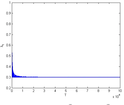
We exemplify the proof above using an example. Assume w1 = 30,PMi=1wi = 100, Si = 1.

k=b₁₀₀T c. The target output rate is w1

PM

i=1wi = 0.3.

According to proof above, N1(0, T) is expressed by the following two expressions.

λ1 = 1×

N1(0, T) T = 1−

70 T b

T

100c, when100b T

100c ≤T ≤100b T

100c+ 30

λ1 = 1×

N1(0, T)

T =

30 T b

T

100c, when100b T

100c+ 30≤T ≤100b T

100c+ 100 limT→∞λ1 =limT → ∞(1−

70 Tb

T

100c) = 0.3, when100b T

100c ≤T ≤100b T

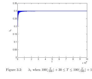
100c+ 30 limT→∞λ1 =limT → ∞(

30 T b

T

100c) = 0.3, when100b T

100c+ 30≤T ≤100b T

100c+ 100 As a result, the output rate converges to 0.3 which is the target output rate. These two equations above are shown in Figures 3.1 and 3.2.

Figure 3.1: λ1 when 100b₁₀₀T c ≤T ≤100b₁₀₀T c+ 30

Lemma 2 Consider a queueing system with a single server of capacity 1 and M queues with

Figure 3.2: λ1 when 100b₁₀₀T c+ 30≤T ≤100b₁₀₀T c+ 100

λi, i= 1, . . . , M, where

λi ≥0, M

X

i=1

λi= 1.

Assume service times for all service domains are 1. Then, in order to achieve target output

rate λi for queue i, the weights for WRR scheduler should be selected proportional to the desired

output rates, i.e.,

wi =L×λi, i= 1, . . . , M, (3.7)

where Lis a constant.

Proof: According to Lemma 1, the output rate for each queue will be a rational number. Since each λi is rational, we can multiply eachλi by a (minimum possible) integerH, such

thatλ0_i =λi×H is integer, and

PM

i=1λ0i=H.

According to Lemma 1, the output rate for service domain iis wi

PM

j=1wj. Let wi

PM

j=1wj

=λi=

λ0_i H

Assume PM

j=1wj =X, whereX is an integer. We have

wi =

λi is an integer, in order to makewi and integer, we need to chooseX such that the fraction

K

K= X H

is an integer. As a result,

wi =K×λ0i=K×H×λi =L×λi

where L is an integer. 4

Lemma 3 Consider two functionsf, gand random variablesv1, v2, v3, v4. LetA=f(v1, v2), B= g(v3, v4). Whenv1, v3 take constant values, andv2 andv4 are independent, the random variables A and B are independent.

Proof: Consider the event

P(A≤a, B ≤b) =P(f(v1, v2)≤a, g(v3, v4)≤b)

Given the condition v1 = c, v3 = d, the event f(c, v2) ≤ a only depends on the random variablev2, the event g(d, v4)≤bonly depends on the random variable v4. Therefore,

P(f(c, v2)≤a, g(d, v4)≤b) =P(f(c, v2)≤a)×P(g(d, v4)≤b) =P(A≤a)P(B ≤b)

According to the definition of independence, Aand B are independent. 4

3.3

Statistical properties of the utilization sequence

For simplicity of notation, in cases where there is no risk of confusion, we drop the dependence of the four variables (i.e.,U(Tk), W(Tk), A(Tk), D(Tk)) on Tk.

Let {Uk

m}∞k=1 denote the sequence of domain m utilizations achieved by the SDA/SAA algorithm, as defined in Equation 3.5. In this section, we establish the statistical properties of this sequence. More specifically, we show that {Uk

m}∞k=1 is a sequence of φ-mixing (see Lemma 5) and identically distributed (see Lemma 6) random variables.

For a random variable sequence {Uk

m}, let F j

i , σ(Umk : i ≤ k ≤ j) be the σ-algebra

generated. Also, let

φ(r), sup

{n,A∈Fn

1,P(A)>0} sup

{B∈Fn+r∞ }

|P(B|A)−P(B)|

Definition: The sequence{Uk

m}is φ-mixing ifφ(r)→0 as r→ ∞.

The definition says that asr → ∞, the supremum over alln, AandBof the term|P(B|A)− P(B)| should go to zero. Loosely speaking, the random variables in a φ-mixing sequence are asymptotically independent.

Lemma 4 Let x be a fixed positive integer. Then there exists an integer y <∞ such that U_mx is independent of {Uk

m}∞x+y.

Proof: The proof is presented in 7 steps. According to the algorithm summary, U_mk is a function of the instantiation matrix Wk−1, queue size matrix Qk−1 of each server from each service domain at time Tk−1, the order Ok−1 of jobs from different service domains in the queues, and a matrix of service times of jobs in different service domains {{S_ij}∞

i=1}Mj=1. Recall that the service times are iid random variables. We can denote

U_mk =f1(Wk−1, Qk−1, Ok−1,{{Sij}∞i=1}Mj=1)

where the function f1 has 4 arguments, Wk−1 is an N ×M matrix, with finite values in each row and column 0≤W_mnk−1 <∞,Qk−1 is anN×M matrix, with finite values in each row and column, order of jobs, and service times. To simplify notation a little, denote a =Wk−1_, b=Qk−1 and c=Ok−1; assume that the scheduler sends jobs to each server in the order from service domain 1 to service domain M. Recall that the servers’ queues are served in a FIFO order. The domain off1 is the set [0,∞)×[0,∞)×...[0,∞); its range is the set [0,1]. We have,

U_mk =f1(a, b, c,{{Sij}∞i=1}Mj=1)

Step1: Assume thatXm(Tx)≥Pm; we will show by contradictions that there always exists

a finitey1 which is independent ofx so that Xm(Tx+y1)≥P_m.

If Xm(Tx)≥Pm, but after y1 periods, Xm(Tx+y1) < P_m, service domain m will be placed in group A. The SDA/SAA algorithm will activate instances of this domain until the condition Xm(Tx+y01)≥P_mis satisfied. Lety01 →y1, so there should always exist ayso thatX_m(T_x+y1)≥ Pm. So service domain m atTx and Tx+y1 will be in the same activation/deactivation group.

There are M service domains; the value of y1 depends actually on the service domain m. Findy1so that all m service domains atTxandTx+y1 will be in the same activation/deactivation groups. Note that this value (which for simplicity of notation we also call y1) only depends on Xm(Tk), which depends on 1_k

Pk

i=1Umi , soy1 is independent of x.

Step2: There always exists a finitey2 so that Wx =Wx+y2.

W is anM ×N matrix, every element of it is an integer which shows how many instances should be activated in a certain server. This integer is finite, as we prove next.

Then service domain m will be in the activation group, and in the following time interval, WRR scheduler will send more traffic from this service domain to the servers. If in subsequent time intervals the utilization Xm(Tx+1) is still less than Pm, then WRR scheduler will send

more and more traffic from this service domain to the servers.

Since service time S_ix ≤M AX, in a finite time this traffic that came before Tx will leave

the queues, and utilization for service domain m will start to increase, until at some time instantT_x+y2, we haveX_m(T_x+y2)> P_m. At this point, the value ofB_m will start to decrease because service domainm is in the deactivation group. So, the elements of W cannot increase to infinity, they have a finite upper bound G. Formally, for any time instantk, we must have 0≤W_nmk ≤G <∞.

Assume that every server cannot have more thanGinstances activated, soW can only have finite values; there always exist infinite numbers ofy2 such thaty2₁, y2₂, y₃2, . . . andWx =Wx+y2i. y2 depends only on W, G but notx.

Step3: There always exists ay3 so that Qx=Qx+y3.

The queue sizes at time Tk−1 depend on the queue sizes atTk−2, the instantiation matrix, the service times of jobs in the queues (in general on {{Sij}∞_i=1}M_j=1), and Ok−2, the order of

jobs from various service domains at Tk−2. More formally, we have

Qk−1=f2(Wk−1, Qk−2, Ok−2,{{Sij}∞i=1}Mj=1)

where the function f2 has 4 arguments, similar to function f1. The domain off2 is [0,∞)× [0,∞)×. . .[0,∞) and its range is [0,∞)×[0,∞)×. . .[0,∞).

Assume the time to send jobs from the gateway to servers is negligible. In a stable system, if we don’t want the queue sizes go to infinity, the input rate should be less than or equal to output rate. During time interval T, the maximum number of jobs can be served in an server is _{M IN}T whereM IN denotes the minimum value that a service time can take.

So Q can only have finite kinds of value, so there always exists infinitely many numbers y₁3, y₂3, y₃3, . . . and Wx=Wx+y3i.y3 depends only on W, G but notx.

Step4: There always exists ay4 _{so that the order of jobs from different service domains at} timex are the same as that atx+y4.

The order of jobs from different service domains depends on how many jobs left for each service domain in each server, and how many jobs from each service domain have been sent during this time interval. We assume that in each server, the jobs from different service domains are sent in the order of SD1, SD2, . . . , SDM, and the server will serve them in a FIFO order.

Step5: In the sequencey₁1, y₂1, y₃1, ..., y₁2, y₂2, y₃2, ...,y₁3, y₂3, y₃3, ..., andy₁4, y₂4, y₃4, ...find the first value thaty_i1 =y_j2=y_h3 =y_l4(=y). Then at time instantsxandx+ywe must haveWx=Wx+y, the same activation/deactivation group, the same queue sizes and order of jobs.

To see that this is the case, suppose to the contrary that no such y exists. Then, at least one ofW, Q and ordering O are different at x and x+y. Order could not be different if W, Q are the same, so at least one ofW, Q are different.

However, W and Q are both N×M matrices with elements bounded by G1, G2. So there are at mostGN₁ ×M×GN₂×M different possible values forW andQ. The (GN₁ ×M×GN₂×M+ 1)th value, therefore, must be the same as one of the previous values.

Step6:U_mx and Umx+y are independent. We have

U_mx =f1(a, b, c,{{Sij}∞i=1}Mj=1) U_mx+y =f1(a, b, c,{{Sij}∞i=1}Mj=1)

All of their arguments are either the same or independent, according to Lemma 3 they are independent. Furthermore, y is independent of x.

Step7: The proof in the previous step involved two time instants x and x+y only; for this step, we need to prove that U_mx is independent of {Uk

m}∞x+y. According to the SDA/SAA

algorithm,

Wk=f3({Xm(Tk)}Mm=1) =f4({Umk}Mm=1,{Xm(Tk−1)}Mm=1)

where f3 has M arguments (the achieved percentiles of allocated time to each service do-main). Its domain is the set [0,1]×[0,1]× · · · ×[0,]) and its range is a M ×N matrix with finite values.

Similarly, f4 has 2M arguments which are the utilization for each service domain and pre-vious actual percentiles of allocated time for each service domain. Its domain is [0,1]×[0,1]× ...×[0,1] and its range is aM×N matrix with finite values. We can write

U_mx+y =f1(Wx+y−1, Qx+y−1, Ox+y−1,{{Sij}∞i=1}Mj=1) U_mx+y+1 =f1(Wx+y, Qx+y, Qx+y,{{Sij}∞i=1}Mj=1)

Wx+y−1 =f3({Xm(Tx+y−1)}Mm=1)

Wx+y =f4({Umx+y}Mm=1,{Xm(Tx+y−1)}Mm=1)

which only depends on random variables defined at the previous time instant.

As a result, Umx+y+1 only depends on Umx+y, which is independent on Umx. Hence {Umk}∞x+y

is independent of Ux

Lemma 5 The sequence of utilizations {Ui

m}∞1 is φ-mixing. Moreover,

P∞

i=1φ(i).5 <∞. Proof: Choose anyn <∞ and choose a setA∈F₁n such that P(A)>0. Then, by Lemma 4, there exists r∗ <∞ such that ∀B ∈F_n∞_+r,|P(B|A)−P(B)|= 0, ∀r > r∗_{. For clarification,}

ncan be viewed asx in 4, andr∗ can be viewed asy in 4. As a result,

φ(r) = sup

{n,A∈Fn

1,P(A)>0} sup

{B∈F∞

n+r}

|P(B|A)−P(B)|= 0

and thus ∀r ≥ r∗, φ(r) = 0. Furthermore, we have that P∞

i=1φ(i).5 < ∞, since φ(r) = 0 when r > r∗. The sum has only only a finite number of nonzero terms. 4

Lemma 6 Consider a given domain m. The random variables U_mi are identically distributed. Moreover, we have

EU_mi =Pm, (3.8)

i.e., the expected value of U_mi equals the target CPU percentile.

Proof: Let F_mi(u) denote the distribution function of U_mi fori= 1,2, . . . Let4 be the set of all initial conditions at the beginning of the time slots.ω ∈ 4stands for the initial condition like initial Wp−1, Wq−1, and Qp−1, Qq−1 and the orders Op−1, Oq−1 in which the jobs from different service domains will be served.

For any ω ∈ 4, Ump, Umq are any two random variable of CPU utilization. Assume that

Wp−1 =Wq−1,Qp−1 =Qq−1 and Op−1 =Oq−1.Fp(u|ω) is identically distributed to Fq(u|ω),

because by a previous definition,

U_mk =f1(a, b, c,{{Sij}∞i=1}Mj=1)

in which the service times are iid random variables. The process of calculating Ump and Umq is

the same (i.e., does not depend onp orq). As a result, for everyu∈R, we have

Fp(u) =

Z

4

Fp(u|ω)P(dω) =

Z

4

Fq(u|ω)P(dω) =Fq(u)

and thus U_mi ’s are identically distributed. We next show thatEU_mi =Pm. Since

cm=E[Umi ] = lim_x→∞

1 x

x

X

i=1

U_mi = lim

it suffices to show that

lim

x→∞Xm(Tx) =Pm

The proof is by contradiction. Assume that the sample average converges to a value not equal toPm, i.e., limx→∞Xm(Tx)6=Pm. Assume that for a positive real number , we have

lim

x→∞Xm(Tx) =Pm+

If at a certain time instant Xm(Tk) = Pm+, the WRR scheduler will send less traffic from

service domain m to the servers, so that after a finite time, when the traffic in the queues is served, the utilization of service domain m will decrease, so that Xm(Tk) will also decrease,

until eventually we have thatXm(Tk)< Pm.

A similar contradiction can be demonstrated with a negative, completing the proof of the

lemma. 4

3.4

The Main Result

Our main result is Theorem 2. It states that the SDA/SAA algorithm achieves any desired percentile utilizations. The result is a direct consequence of the following proposition from [4].

Proposition 1 Let {Zn} be an identically distributed and φ-mixing sequence of random

vari-ables with E[Zn] =c and P∞i=1φ(i).5 <∞, Let Sn=Pni=1Zi. Then

Sn

n →n→∞ c, a.s. (3.9)

Equation 3.9 in the proposition extends the almost sure (a.s.) convergence result of the Strong Law of Large Numbers to sequences of dependent random variables.

Theorem 1 Let Pm, m = 1,2, . . . , M, denote arbitrary target CPU utilizations, where 0 ≤

Pm≤1andPmPm = 1. LetXm(Tk)denote the utilization achieved by the SDA/SAA algorithm

up until time Tk. ThenXm(Tk) converges almost surely to Pm:

Xm(Tk)→Tk→∞ Pm, a.s., m= 1,2, . . . , M. (3.10)

Proof: Lemma 6 proves that the U_mi random variables are identically distributed with E[Um] =Pm; Lemma 5 proves that{Umi }∞i=1 isφ-mixing, with

P∞

i=1φ(i).5<∞;Xm(Tk) is the

sample average of random variable sequence{Ui

m}∞i=1. As a result, according to Proposition 1,

3.5

Extended Results

In this extension, we consider up and down tolerances that may have nonzero values.

Theorem 2 Let Pm, m = 1,2, . . . , M, denote arbitrary target CPU utilizations, where 0 ≤

Pm≤1andPmPm = 1. LetXm(Tk)denote the utilization achieved by the SDA/SAA algorithm

up until time Tk. Then

Pm−DT < lim

k→∞Xm(Tk)< Pm+U T (3.11)

Proof: There are 4 possible cases for the limiting value of Xm(Tk):

(a) Xm(Tk) converges to a constant cm, wherecm ∈[Pm−DT, Pm+U T].

(b) Xm(Tk) converges to a random variablePm0 , wherePm0 ∈[Pm−DT, Pm+U T].

(c) Xm(Tk) doesn’t converge; instead it oscillates between [Pm−DT, Pm+U T].

(d) Xm(Tk) doesn’t converge; instead it oscillates outside [Pm−DT, Pm+U T].

Case (a) is not possible because of this counter-example: if [Pm−DT, Pm+U T] = [0%,100%],

then utilization will only depend on the initial value ofB, which is a random variable, and service times which are iid random variables. Utilization can not converge to a constant.

Case (d) is not possible either; since

Xm(Tk) =

1 kN

N

X

n=1 Unm+

k−1

k Xm(Tk−1)

we can easily see thatXm(Tk) cannot jump from a value greater thanPm+U T to a value less

thanPm−DT. Indeed, as k→ ∞, _kN1 PN_n=1Unm →0, and k−_k1 →1. IfXm(Tk−1)> Pm+U T,

then _kN1 PN

n=1Unm needs to be larger thanU T +DT, which is not possible.

Moreover, note thatXm(Tk) cannot always stay outside [Pm−DT, Pm+U T]. If at a certain

time we haveXm(Tk) =Pm+U T+, the WRR scheduler will send less instances from service

domain m to the appliances, so that after a finite time, when the requests of the domain are served, the utilization of service domain m will decrease and Xm(Tl) will also decrease, until

Xm(Tl)< Pm+U Tm.

As a result, the only possible cases are either (b) or (c); in both, the utilizations reach their

Chapter 4

Conclusion and Future Work

4.1

Summary and Conclusion

In this thesis, we have studied a problem in the space of service differentiation in Service Oriented Architecture environments. In such environments, service classes (service domains) compete for a share of available CPU resources. The allocation of such resources is often gov-erned by Service Level Agreements (SLA). The specific SLA we have considered calls for allo-cating a given percentile Pm of CPU time to service domainm. The SDA/SAA algorithm has

been proposed in the past as an efficient, feedback-based method to guarantee this SLA. The main contribution of this thesis is a theoretical proof that the SDA/SAA algorithm is capable of achieving the SLA under a variety of realistic assumptions. This result was stated as Theo-rem 1 in Section 3.4. The proof utilizes the theory of φ-mixing random processes to study the convergence properties of the sequences of service domain utilizations. These processes provide a convenient model for capturing the dynamics of dynamic control algorithms which rely on processing feedback in a history- (but not time-)dependent fashion. When the tolerance param-eters allowed in the SDA/SAA algorithm are equal to zero (U T =DT = 0) and the buffers are assumed saturated with traffic (i.e., infinite queue sizes), the utilizations converge almost surely to the target CPU utilizations specified in the SLA. When a tolerance parameter is not equal to zero, it is not known whether the utilizations oscillate or converge; however, the algorithm will guarantee that they remain in the range [Pm−DT, Pm+U T] (as it would have been expected).

4.2

Future Work

The case of unsaturated buffers presents an interesting case for future work. Suppose that arrivals to service domainmoccur at a rateλm. There are two possibilities to be considered in

case is interesting for future work; it is formally characterized by the condition λm×ESm <

Pm −DT (DT may or may not be 0). In this case, according to the SDA/SAA algorithm

REFERENCES

[1] Heiko Ludwiq Asit Dan and Giovanni Pacifici. Web service differentiation with service level agreements. IBM developerWorks, 2003.

[2] Yvonne Balzer. Improve your soa project plans. IBM, 2004.

[3] Keerthana Boloor. Multi-point to Single-point Service Traffic Shaping. PhD thesis, North Carolina State University, 03 2009.

[4] Ernst Eberlein and Murad S. Taqqu. Dependence in probability and statistics. Birkhauser Boston, Inc, Bostan, MA, 1986.

[5] Hugo Haas and Allen Brown. Web services glossary. W3C Working Group Note, 2004.

[6] Mursalin Habib. Provisioning algorithm for service differentiation in middleware appliance clusters. PhD thesis, North Carolina State University, 03 2009.

[7] Raghu R. Kodali. An introduction to soa. JavaWorld, 2005.

[8] Lafteris Mamatas and Vassilis Tsaoussidis. Differentiating services with non-congestive queuing(ncq). 2008.

[9] A. K. Parekh and R. G. Gallager. A generalized processor sharing approach to flow con-trol in integrated services networks: the single-node case. IEEE/ACM Transactions on Networking, 1993.

[10] David Sprott and Lawrence Wilkes. Understanding service-oriented architecture. CBDI Forum, 2004.

Appendix A

CASTS Algorithm Proof

In this appendix we provide a proof that CASTS Algorithm works. For more details on CASTS and the problem it solves in SOA, see [3].

A.1

Problem Definition

Service providers within an enterprise network are often governed by Client Service Con-tracts (CSC) that specify, among other constraints, the rate at which a particular service in-stance may be accessed. The main challenge is to enforce the global traffic contract by taking local actions at each appliance [3], which means the appliances locally shape the service requests to respect the global contract. The need exists for a dynamic, measurement-based service traffic shaping algorithm which respects the CSC and where credits are assigned to the middleware appliances (entry points) based on the current state of the system.

A.2

Description of CASTS Algorithm and Manual Static

Algo-rithm

A.2.1 CASTS Algorithm Introduction

is slotted into K equal subperiods during which the updating of the credits take place at each appliance by exchanging their respective queue details and current credit assignment.

The CASTS algorithm is a decentralized algorithm for service traffic shaping in middleware appliances. In centralized implementations, appliances send their measurements to the central point (appliance). In decentralized ones, the middleware appliances (entry points) exchange information about their queues (an indication of their input rate) with their peer appliances every subperiod within the observation interval specified by the CSC.

A.2.2 Notations and clarifications for the proof X is the number of requests per unit time.

T is the total number of time periods. B is the total number of appliances. K is the total number of subperiods. Y is the number of incoming requests.

When in the kth subperiod, the maximum number of requests theith appliance can handle is xi(k), the number of incoming requests is Yi(k), the actual number of requests that were

handled is ri(k), the queue length of ith appliance afterkth subperiod isQi(k), and R(k) is the

total number of documents sent by all appliances after kth subperiod.

In order to distinguish the CASTS algorithm from the static one, all variables refering to the static algorithm are denoted with a bar (for example ¯x.

When run on the appliances, the CASTS algorithm triggers the adaptation phase at the beginning of each subperiod where the credit assigned to the appliance is updated based on the current state of the system; during the remaining duration of the subinterval, the appliance is in the measurement phase, collecting the actual number of service requests sent to the host. The credits available for the appliance to use during the subperiod k is xi(k). During the

measurement subperiod k, each appliance measures the actual number of documents ri(k) it

was able to send to the service host. If there was not enough traffic entering the appliance, ri(k) could be less that xi(k). Otherwise, ri(k) should be equal to xi(k). Each appliance also

measures the queue size,Qi(k), at the entry points. The number of requests in the queues of the

appliance is an indication of the input rate at each appliance and will be used to determine the credits allotted to the appliance. In this way, credit assignment is performed under a weighted strategy.

At the end of the measurement subperiodk, each appliance broadcasts to all other appliances the valuesri(k) andQi(k); after receiving feedback from all other appliances, applianceiupdates

its local shaping ratexi(k+ 1) during the adaptation phase as shown in the next subsection.

amount of credits assigned to the appliances at each subinterval is always smaller or equal to the remaining allowed number of documents:

X

1≤i≤B

xi(k)≤X×T−R(k)

where R(k) is the total number of documents sent by all appliances during the previous sub-periods.

A.2.3 CASTS Algorithm

Input:k, (when 1< k≤K) rj(k−1) and Qj(k−1) , wherej = [1, .., B], j6=i

Output: new count xi(k)

ifk= 1, then xi(k)← X_B×T

else

r(k−1) =PB

j=1rj(k−1)

R(k−1) =Pk−1

n=1r(n) ifR(k−1)< X×T, then

D←X×T −R(k−1) ifPB

n=1Qn(k−1) = 0, then xi(k)← bD÷Bc

else

xi(k) =bDP×BQi(k−1) n=1(k−1) c end if

else

xi(k)←0

end if end if

ifYi(k)≥xi(k), then

ri(k)←xi(k)

Qi(k)←Yi(k)−xi(k)

else

ri(k)←Yi(k)

Qi(k)←0

A.2.4 Manual Static Allocation

The allowed number of requestsxi from each of the appliances is the same

¯ xi =b

X×T B c

If the total period is divided into K sub-periods, then in each sub-period, the length of the sub-period will beT ÷K, the allowed number of requests will be

¯

xi(k) =b

X×T K×Bc

A.3

Proof

In order to prove that the CASTS algorithm respects the SAR, we should prove thatR(k)≥ ¯

R(k) (almost surely). We prove the result first for the special case of B = 1, K = 1; we then relax this assumption.

A.3.1 Case B = 1, K = 1 In this case, we can write:

x(1) =bX×T

B c,x(1) =¯ b X×T

K×Bc=bX×Tc

The actual number of requests that is handled is the minimum ofxi(k) andYi(k). In this case,

r(1) = min(x(1), Y(1)) = min(bX×Tc, Y(1)),r(1) = min(¯¯ x(1), Y(1)) = min(bX×Tc, Y(1))

Since there is no previous sub-period, the actual number of requests that were handled in previous sub-periods are 0. Then,

R(1) =

k

X

n=1

r(n) =r(1) = min(bX×Tc, Y(1)),R(1) =¯

k

X

n=1 ¯

r(n) = ¯r(1) = min(bX×Tc, Y(1))

Therefore, R(1) = ¯R(1) and the result holds.

A.3.2 Case B 6= 1, K = 1 In this case, we can write

xi(1) =b

X×T

B c,x¯i(1) =b X×T

ri(1) = ¯ri(1) = min(b

X×T

B c, Yi(1))

r(1) =

B

X

i=1

ri(1), ¯r(1) = B

X

i=1 ¯ ri(1)

sor(1) = ¯r(1). As stated before,R(1) = ¯R(1) and the result holds.

A.3.3 Case B = 1, K 6= 1

In this case, we use induction on the subperiodk; when k= 1, we can write

x(1) =bX×Tc,x(1) =¯ bX×T K c Since K≥2 we have that x(1)≥2×x(1).¯

r(1) = min(x(1), Y(1)),r(1) = min(¯¯ x(1), Y(1))

Since x(1)≥2×x(1), we have that¯ r(1)≥r(1), so¯ R(1)≥R(1), and the result holds.¯

Consider the following three cases. Sincex(1)≥2×x(1), Y(1) can be in 3 different regions¯ based on the relationship betweenx(1) and ¯x(1):Y(1)≥x(1)≥x(1),¯ x(1)≥Y(1)≥x(1), and¯ x(1)≥x(1)¯ ≥Y(1).

1. Y(1)≥x(1)≥x(1)¯

Since Qi(k) =Yi(k)−xi(k),Q¯i(k) =Yi(k)−x¯i(k)

Q(1)6= 0,Q(1)¯ 6= 0

2. x(1)≥Y(1)≥x(1)¯

Q(1) = 0,Q(1)¯ 6= 0

3. x(1)≥x(1)¯ ≥Y(1)

Q(1) = 0,Q(1) = 0¯

Assume now that in the (k−1)th sub-period, we haveR(k−1)≥R(k¯ −1). There are also three cases based on the queue length, similar to the k= 1 case.

1. Q(k−1)6= 0,Q(k¯ −1)6= 0

2. Q(k−1) = 0,Q(k¯ −1)6= 0

Consider what happens during the kth subperiod, next.

1. CaseQ(k−1)6= 0,Q(k¯ −1)6= 0. Since under CASTS algorithm the maximum number of requests it sends is the total number that left, so if the queue is not 0, it must have used up all credits available. Then

x(k) = 0,x(k) =¯ bX×T K c

r(k) = 0,r(k)¯ ≤ bX×T K c R(k) =bX×Tc,R(k)¯ ≤K× bX×T

K c ≤ bX×Tc soR(k)≥R(k), and the result holds.¯

2. CaseQ(k−1) = 0,Q(k¯ −1)6= 0. In this case, we can write

x(k) =bX×T−R(k−1),x(k) =¯ bX×T K c r(k) = min(bX×T −R(k−1)c, Y(k))

Now, if ¯Q(k−1)≥x(k), we have¯ ¯

r(k) = ¯x(k)≤Q(k¯ −1)

becauseR(k−1) +Q(k−1) = ¯R(k−1) + ¯Q(k−1) R(k−1) + 0≥R(k¯ −1) + ¯r(k) = ¯R(k)

soR(k)≥R(k), and the result holds.¯

If, on the other hand, ¯Q(k−1)<x(k), then we can write¯ ¯

r(k) = min(bX_K×Tc −Q(k¯ −1), Y(k)) + ¯Q(k−1) Suppose that bX×T−R(k−1)c ≥ bX×T

K c −Q(k¯ −1). Since

R(k−1) +Q(k−1) = ¯R(k−1) + ¯Q(k−1)and Q(k−1) = 0

we have

R(k) =R(k−1) +r(k) =R(k) + min(bX×T−R(k−1)c, Y(k))

¯

= ¯R(k−1) + ¯Q(k−1) + min(bX×T

K −Q(k¯ −1), Y(k))

Therefore, R(k)≥R(k), and the result holds.¯

Suppose next that bX×T−R(k−1)c<bX×T

K c −Q(k¯ −1).

We have to consider again two cases. First, ifY(k)≥ bX×T −R(k−1)c, then R(k) =bX×Tc, ¯R(k)≤K× bX_K×T ≤ bX×Tc

so R(k)≥R(k), and the result holds.¯ Second, ifY(k)<bX×T−R(k−1)c, then

r(k) =Y(k), ¯r(k) =Y(k) +Q(k−1) R(k) = ¯R(k), and the result holds.

3. In caseQ(k−1) = 0,Q(k¯ −1) = 0, we can write x(k) =bX×T−R(k−1)c, ¯x(k) =bX_K×Tc

r(k) = min(bX×T −R(k−1)c, Y(k)), ¯r(k) = min(bX×T

K c, Y(k))

Now, if bS×T−R(k−1)c ≥ bX×T

K c, then

r(k)≥r(k)¯

soR(k)≥R(k), and the result holds.¯ IfbS×T−R(k−1)c ≤ bX_K×Tc, then

ifY(k)≥ bX×T−R(k−1)c, then R(k) =bX×Tc

¯

R(k)≤K× bX_K×Tc ≤ bX×Tc so R(k)≥R(k), and the result holds.¯ ifY(k)<bX×T−R(k−1)c, then

r(k) = ¯r(k) =Y(k)

so R(k)≥R(k), and the result holds.¯ In all cases above, the result holds.

A.3.4 The general case B 6= 1, K 6= 1

When B = 1, the result holds, i.e, it holds for each appliance. Treat every appliance indepen-dently, and substitute xi(k), ri(k), Qi(k), Ri(k) for every x(k), r(k), Q(k), R(k) under both

CASTS algorithm and the static algorithm in (3). We can get

Since R(k) =PB

i=1Ri(k), and ¯R(k) =PBi=1R¯i(k), we can get

R(k)≥R(k)¯