Orientational distribution functions and order parameters in "de Vries"-type smectics : a simulation study

smectics - a simulation study

Frank Jenz,1 _{Mikhail A. Osipov,}2_{Stefan Jagiella,}1 _{and Frank Giesselmann}1,a)

1)

Institute of Physical Chemistry, Pfaffenwaldring 55, University of Stuttgart, Stuttgart Germany

2)_{Department of Mathematics and Statistics, G1 1XH, University of Strathclyde,}

Glasgow UK

(Dated: 13 September 2016)

Simple smectic A liquid crystal phases with different types of prescribed orientational distribution functions have been simulated and compared in order to study the possibility to distinguish between the Maier-Saupe

type and cone-like orientational distributions using the popular method of Davidson et al. This method

has been used to extract the orientational distribution functions from simulated diffraction patterns, and the results have been compared with actual distribution functions which have been prescribed during simulations. It has been shown that it is indeed possible to distinguish between these two qualitatively different types of orientational distribution already from the shape of the 2D diffraction pattern. Moreover, typical experimental diffraction patterns for ”de Vries”-type smectic liquid crystals appear to be close to the ones which have been simulated using the prescribed Maier-Saupe orientational distribution function.

Keywords: Liquid Crystals, X-ray Diffraction, Order Parameter, Orientational Distribution Function

I. INTRODUCTION

There exist a number of experimental techniques to de-termine the orientational order parameters which spec-ify the degree of the orientational order of anisotropic molecules in various liquid crystal phases. In particular,

both the second rank orientational order parameter S2

and the fourth rank order parameter S4 can be

deter-mined from 2D X-ray diffraction patterns as was

origi-nally suggested by Leadbetter and Norris1_{. A more}

re-fined method has later been suggested by Davidson,

Pe-termann and Levelut2 _{and this procedure has been used}

by different authors to measure the order parameters of

the nematic, smectic A and smectic C phases3–6.

The method of Davidson et al. is based on a number

of approximations and it is not cleara priori what is the

accuracy of the results even though the values of S2 are

known to correlate well with the results obtained by other experimental techniques like NMR, via dielectric

relax-ation, optical birefringence or Raman spectroscopy7–12_.

In a previous paper we have used computer simulations

to evaluate the accuracy of this method13_{. We could}

show that the method of Davidson et al. is reliable but, due to translational correlations between orientationally

ordered molecules14, which are not taken into account,

it slightly underestimates the order parameterS2by

ap-prox. 0.05.

One notes that all phases, simulated in13_{, are}

charac-terised by a Maier-Saupe like orientational distribution function (Fig. 1a) and rather high values of the

orien-tational order parameter S2. On the other hand, it is

very interesting to investigate if the method of David-son et al. can be used to distinguish between smectic

a)_{[email protected]}

liquid crystals with different shapes of the orientational distribution function. In particular, starting from the

original works of de Vries15,16some authors assume that

in the so-called smectics A of ”de Vries” type the long molecular axes are tilted by a more or less constant angle

with respect to the smectic layer normal17_{. This}

corre-sponds to the so-called hollow-cone orientational distri-bution shown schematically in Fig. 1c. A more general orientational distribution of this kind corresponds to the so-called diffuse cone model presented in Fig. 1b.

A comparison of the initial orientational distribution functions of qualitatively different shapes with the corre-sponding functions extracted from the simulated diffrac-tion patterns can be undertaken if the actual orienta-tional distribution is fixed during the simulations of the structure factor and the corresponding diffraction pat-tern. In this paper we undertake such simulations using a very simple model of the smectic A phase with per-fect smectic order, prescribed values of the orientational variables, which correspond to a given shape of the distri-bution function, and 2D positional freedom of molecular centres of mass inside a given smectic layer.

So far, the existing experimental data do not pro-vide conclusive epro-vidence whether or not these hypotheti-cal cone-like distributions really exist in ”de Vries”-type smectics18–21_{. This knowledge is however essential to}

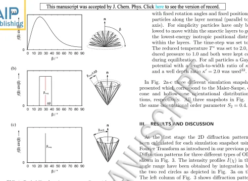
βavg βavg ±Δβ (a) (b) (c) β n 0

0 10 20 30 40 50 60 70 80 90

f ( β ) sin( β )

β/°

0

0 10 20 30 40 50 60 70 80 90

f ( β ) sin( β )

β/°

0

0 10 20 30 40 50 60 70 80 90

f ( β ) sin( β )

β/°

βavg

Δβ

βavg

n

n

FIG. 1. Probability functions corresponding to the three ori-entational distribution functions: (a) Maier-Saupe distribu-tion. (b) Diffuse-Cone distribudistribu-tion. (c) Hollow-Cone distri-bution.

II. SIMULATION PROCEDURE

The smectic A phases composed of uniaxial particles with prescribed orientational distribution function and perfect translational order has been simulated. In this

case the translational order parameter Σ = 1.0 and the

instant orientation of a particle is specified by the polar

angleθ with respect to the smectic layer normal (or the

molecular tilt angle) and the azimuthal angle in the plane of the layers. Then the simulation snapshots have been generated by the following steps:

1. The molecular tilt angles of the particles in the sim-ulation box have been set in accordance to the pre-scribed ODF.

2. Azimuthal angles of all particle have been set

ran-domly between 0 and 360◦.

3. Position of each particle in the simulation box was set randomly. Overlapping of particles has been thereby prevented.

4. The simulation has been equilibrated by Molecu-lar Dynamics (MD) using 200000 integration steps

with fixed rotation angles and fixed positions of the particles along the layer normal (parallel to the z-axis). For simplicity particles have only been al-lowed to move within the smectic layers to generate the lowest-energy isotropic positional distribution within the layers. The time-step was set to 0.001.

The reduced temperatureT∗ was set to 2.0, the

re-duced pressure to 1.0 and both were kept constant during equilibration. For all particles a Gay-Berne

potential with a length-to-width ratio of κ = 4.0

and a well depth ratioκ′ = 2.0 was used22.

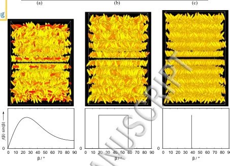
In Fig. 2a-c three different simulation snapshots are presented which correspond to the Maier-Saupe, diffuse-cone and hollow-diffuse-cone orientational distribution func-tions, respectively. All three snapshots in Fig. 2 have the same orientational order parameterS2= 0.4.

III. RESULTS AND DISCUSSION

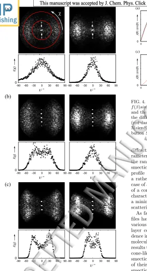
At the first stage the 2D diffraction patterns have been calculated for each simulation snapshot using Fast Fourier Transform as introduced in our previous paper13. Diffraction patterns for three different types of ODFs are shown in Fig. 3. The intensity profilesI(χ) in the wide angle range have been obtained by integration between the two red circles as depicted in Fig. 3a on the left. The left column of Fig. 3 shows diffraction patterns for

S2= 0.4 while the right column corresponds to a second

simulation series withS2= 0.7.

One notes that the diffraction pattern obtained from simulations of smectic A phases with different types of prescribed orientational distribution function are quali-tatively different. In particular, the diffraction pattern, which corresponds to the Maier-Saupe ODF (Fig. 3a), is characterised by only one maximum in the wide angle range, and the peak is becoming more narrow with in-creasingS2. In contrast, for the smectic A phase with the

diffuse-cone distribution (Fig. 3b) one obtains a broad, plateau-like maximum. This maximum becomes sharper

for higher S2 and in this case the pattern is closer to

the one obtained for smectics with the Maier-Saupe dis-tribution. Finally the diffraction pattern for the system with the hollow-cone ODF (Fig. 3c) is characterised by two distinct maxima which are visible for both small and largeS2.

It should be noted also that typical experimentally measured 2D X-ray diffraction patterns3,17,23,24_{are closer}

to our simulated patterns obtained for smectics A with the Maier-Saupe ODF.

Another interesting observation in the diffraction pat-terns of Fig. 3 is that - even though the translational

order parameter is fixed to Σ = 1.0 in all simulations

- the intensity ratios of the smectic layer peaks change with both, the shape of the ODF and the orientational

order parameterS2 in a non-obvious way. This

(a) (b) (c)

0

0 10 20 30 40 50 60 70 80 90

β/°

0

0 10 20 30 40 50 60 70 80 90

β/°

0

0 10 20 30 40 50 60 70 80 90

β/°

f

(

β

) sin(

β

)

FIG. 2. Top: Simulation snapshots for (a) Maier-Saupe distribution , (b) Diffuse-Cone distribution and (c) Hollow-Cone distribution of polar angles of rod-like particles, respectively. Red particles are perpendicular and yellow particles are parallel to the director. Bottom: Prescribed orientational distribution functions used in the simulation above. All three depicted snapshots are characterised by the same nematic order parameterS2= 0.4.

parameters such as ⟨P2(cosβ) cos(2πz/d)⟩as it was

re-cently pointed out by Palermoet al.25

At the second stage the orientational distribution func-tion was extracted from the calculated diffracfunc-tion

pat-terns using the method of Davidson et al. The results,

presented in Fig. 4, have then been compared with the corresponding prescribed ODFs. In the case of smectics A with the Maier-Saupe distribution function the ODF is reproduced very well. In contrast, for systems with cone-like distributions the agreement between the prescribed and the calculated ODFs is rather poor which is related to the cosine series expansion employed in the method

of Davidson et al. The cone-like distribution functions

can adequately be described only using a large number of terms in the series expansion.

Finally we have calculated the values of the orienta-tional order parameter S4 for all three types of the

ori-entational distribution function. In Figure 5 we depict the error inS4obtained by subtracting the values ofS4,

calculated directly from the snapshots, from the values

of S4, extracted from the simulated diffraction patterns

(Fig. 3) using the method of Davidson et al. One can

readily see that for smectics with Maier-Saupe like dis-tribution the deviation is close to zero, and hence the

calculation of the order parameterS4 via the method of

Davidsonet al. is reliable. In contrast, for systems with cone-like distributions the calculated values ofS4are not

very reliable which may be due to truncation errors in the expansion of the wide-angle intensity profile in the cosine series.

IV. CONCLUSIONS

In this paper we have calculated the orientational dis-tribution functions and the orientational order

param-eters S2 and S4, using the method of Davidson et al.,

from the diffraction patterns which have been simulated for a simple smectic A phase with prescribed orienta-tional distribution of molecules. We have used the ori-entational distribution, which corresponds to the Maier-Saupe model, typical for conventional smectics A and the cone-like distributions, which are sometimes assumed to characterize smectics A of the ”de Vries” type.

χ

(a)

-90 -60 -30 0 30 60 90

χ/°

-90 -60 -30 0 30 60 90

χ/°

I ( χ ) 0 (b)

-90 -60 -30 0 30 60 90

χ/°

-90 -60 -30 0 30 60 90

χ/°

I ( χ ) 0 (c)

-90 -60 -30 0 30 60 90

χ/°

-90 -60 -30 0 30 60 90

χ/°

I

(

χ

)

0

FIG. 3. 2D Diffraction patterns of simulations with prescribed orientational distribution function. The wide-angle intensity profiles I(χ) are depicted below the related diffraction pat-terns. Left: Orientational order parameterS2 = 0.4. Right:

Orientational order parameterS2= 0.7. (a) Maier-Saupe

dis-tribution (Fig. 2a). The red circles define the region where theI(χ)-profile has been calculated. (b) Diffuse-Cone distri-bution (Fig. 2b). (c) Hollow-Cone distridistri-bution (Fig. 2c).

f ( ) sin( ) 0 0 f ( ) sin( ) (a) (b) (c) (d)

0 15 30 45 60 75 90

/° Prescribed Diffraction pattern

0 15 30 45 60 75 90

/°

0 15 30 45 60 75 90

/°

0 15 30 45 60 75 90

/°

FIG. 4. Comparison of the orientationl distribution functions

f(β)sin(β), prescribed during the simulations (black line), and the corresponding distribution functions extracted from the diffraction patterns using the method of Davidsonet al.

(red dashed line). (a) Maier-Saupe distributionS2= 0.4. (b)

Maier-Saupe distributionS2 = 0.7. (c) Diffuse-Cone

distri-butionS2= 0.4. (d) Hollow-Cone distributionS2= 0.4.

diffraction pattern provided the orientational order pa-rameter is not too high, i.e. S2 <0.7. In particular, in

the range ofS2 between 0.4 and 0.6, which is typical for

smectics A of ”de Vries” type, the azimuthal intensity profile I(χ) of the diffuse wide-angle scattering possess a rather pronounced and well-defined maximum in the case of a Maier-Saupe type distribution, while in the case of a cone-like distribution the same diffraction profile is characterized by a rather flat plateau or sometimes even a minimum at small azimuthal angles with a significant scattering of data in that region.

As far as we know, the latter type of diffraction pro-files have experimentally never been observed so far for various ”de Vries”-type smectics with anomalously weak

layer contraction. Thus there is no experimental

evi-dence in favour of a cone-like orientational distribution of molecules in smectics of ”de Vries” type. The simulation results thus give strong support to earlier claims18–21_that

cone-like distributions do not exist in ”de Vries”-type smectics even though they could nicely explain many of their striking properties, in particular the absence of smectic layer contraction in the tilting transition to smec-tic C.

A good agreement between the initial values of the

order parameterS2and the corresponding values,

calcu-lated from the diffraction patterns, has been found for all three types of the orientational distribution consid-ered. In all cases the method slightly underestimates the

value ofS2 (by approximately 0.04) which is related to

the contribution of the translational fluctuations between orientationally ordered molecules14_.

In contrast, the calculated values of the order

param-eterS4 are less reliable as the discrepancy between the

(a)

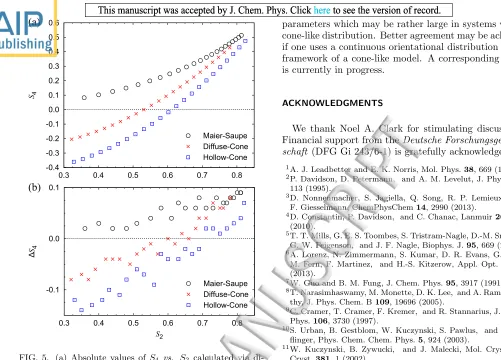
(b)

0.3 0.4 0.5 0.6 0.7 0.8

S4 Maier-Saupe Diffuse-Cone Hollow-Cone -0.1 0.0 0.1

0.3 0.4 0.5 0.6 0.7 0.8

∆ S4 S 2 Maier-Saupe Diffuse-Cone Hollow-Cone

FIG. 5. (a) Absolute values of S4 vs. S2 calculated via

di-agonalisation of the order tensor. In case of Maier-Saupe ODF,S4 is positive over the total range of S2. For

Diffuse-Cone distributions, S4 decreases faster with decreasing S2

and becomes negative below S2 = 0.52. For Hollow-Cone

distributions, S4 decreases even faster with decreasing S2

than in the Diffuse-Cone case and becomes negative already below S2 = 0.7. (b) Deviation of higher order parameter

S4, calculated from the simulated diffraction patterns using

the method of Davidson et al., from the value of S4

calcu-lated directly from simulations for smectics A with Maier-Saupe, Diffuse-Cone and Hollow-Cone orientational distribu-tion funcdistribu-tions. Note that the error is small in the case of Maier-Saupe ODF.

thus comparable to the size of S4 itself. In particular,

the relative deviation is particularly large for hypotheti-cal smectics A with a cone-like distribution in the region whereS4is close to zero. This may be related to the

trun-cation errors. Indeed, both hollow-cone and diffuse cone orientational distributions are discontinuous and thus can be correctly represented by a Fourier series only if a large amount of terms is taken into account. In other words,

a large discrepancy in the values of S4 may represent a

sum of discrepancies in the values of other higher order

parameters which may be rather large in systems with a cone-like distribution. Better agreement may be achieved if one uses a continuous orientational distribution in the framework of a cone-like model. A corresponding study is currently in progress.

ACKNOWLEDGMENTS

We thank Noel A. Clark for stimulating discussions.

Financial support from theDeutsche

Forschungsgemein-schaft (DFG Gi 243/6-1) is gratefully acknowledged.

1_{A. J. Leadbetter and E. K. Norris, Mol. Phys.38, 669 (1979).} 2_{P. Davidson, D. Petermann, and A. M. Levelut, J. Phys. II5,}

113 (1995).

3_{D. Nonnenmacher, S. Jagiella, Q. Song, R. P. Lemieux, and}

F. Giesselmann, ChemPhysChem14, 2990 (2013).

4_{D. Constantin, P. Davidson, and C. Chanac, Lanmuir26, 4586}

(2010).

5_{T. T. Mills, G. E. S. Toombes, S. Tristram-Nagle, D.-M. Smilgies,}

G. W. Feigenson, and J. F. Nagle, Biophys. J.95, 669 (2008).

6_{A. Lorenz, N. Zimmermann, S. Kumar, D. R. Evans, G. Cook,}

M. Fern, F. Martinez, and H.-S. Kitzerow, Appl. Opt.22, E1 (2013).

7_{W. Guo and B. M. Fung, J. Chem. Phys.95, 3917 (1991).} 8_{T. Narasimhaswamy, M. Monette, D. K. Lee, and A.}

Ramamoor-thy, J. Phys. Chem. B109, 19696 (2005).

9_{C. Cramer, T. Cramer, F. Kremer, and R. Stannarius, J. Chem.}

Phys.106, 3730 (1997).

10_{S. Urban, B. Gestblom, W. Kuczynski, S. Pawlus, and A.}

Wr-flinger, Phys. Chem. Chem. Phys.5, 924 (2003).

11_{W. Kuczynski, B. Zywucki, and J. Malecki, Mol. Cryst. Liq.}

Cryst.381, 1 (2002).

12_{A. Sanchez-Castillo, M. A. Osipov, and F. Giesselmann, Phys.}

Rev. E81, 021707 (2010).

13_{F. Jenz, S. Jagiella, M. A. Glaser, and F. Giesselmann,}

ChemPhysChem17, 1568 (2016).

14_{M. A. Osipov and B. I. Ostrovskii, Cryst. Rev.3, 113 (1992).} 15_{A. de Vries, A. Ekachai, and N. Spielberg, Mol. Cryst. Liq. Cryst.}

49, 143 (1979).

16_{A. de Vries, J. Chem. Phys.71, 25 (1979).}

17_{H. Yoon, D. M. Agra-Kooijman, K. Ayub, R. P. Lemieux, and}

S. Kumar, Phys. Rev. Lett.106, 087801 (2011).

18_{J. P. F. Lagerwall and F. Giesselmann, ChemPhysChem7, 20}

(2006).

19_{S. T. Lagerwall, P. Rudquist, and F. Giesselmann, Mol. Cryst.}

Liq. Cryst510, 148 (2009).

20_{A. Sanchez-Castillo, M. A. Osipov, S. Jagiella, Z. H. Nguyen,}

M. Kaspar, V. Hamplova, J. Maclennan, and F. Giesselmann, Phys. Rev. E: Stat., Nonlinear, Soft Matter Phys. 85, 061703 (2012).

21_{Y. Yamada, A. Fukuda, J. K. Vij, N. Hayashi, and T. Ando,}

Liq. Cryst.4, 864 (2015).

22_{J. G. Gay and B. J. Berne, J. Chem. Phys.74, 3316 (1981).} 23_{C. P. J. Schubert, A. Bogner, J. H. Porada, K. Ayub, T. Andrea,}

F. Giesselmann, and R. P. Lemieux, J. Mater. Chem. C2, 4581 (2014).

24_{K. M. Mulligan, A. Bogner, Q. Song, C. P. J. Schubert, F.}

Gies-selmann, and R. P. Lemieux, J. Mater. Chem. C2, 82708276 (2014).

25_{M. F. Palermo, A. Pizzirusso, L. Muccioli, and C. Zannoni, J.}

β

avg

β

±

Δβ

(a)

(b)

(c)

β

n

0

0 10 20 30 40 50 60 70 80 90

f

(

β

) sin(

β

)

β

/

°

0

0 10 20 30 40 50 60 70 80 90

f

(

β

) sin(

β

)

β

/

°

0

0 10 20 30 40 50 60 70 80 90

f

(

β

) sin(

β

)

β

/

°

β

Δβ

β

n

(a)

(b)

(c)

0

0

10 20 30 40 50 60 70 80 90

β

/

_°

0

0

10 20 30 40 50 60 70 80 90

β

/

_°

0

0

10 20 30 40 50 60 70 80 90

β

/

_°

f

(

β

) sin(

β

χ

(a)

-90

-60

-30

0

30

60

90

χ

/

_°

-90

-60

-30

0

30

60

90

χ

/

_°

I

(

χ

)

0

(b)

-90

-60

-30

0

30

60

90

χ

/

_°

-90

-60

-30

0

30

60

90

χ

/

_°

I

(

χ

)

0

(c)

-90

-60

-30

0

30

60

90

χ

/

_°

-90

-60

-30

0

30

60

90

χ

/

_°

I

(

χ

)

f

(

) sin(

)

0

0

f

(

) sin(

)

(a)

(b)

(c)

(d)

0

15

30

45

60

75

90

/

°

Prescribed

Diffraction pattern

0

15

30

45

60

75

90

/

°

0

15

30

45

60

75

90

/

°

0

15

30

45

60

75

90

(b)

-0.4

-0.3

-0.2

-0.1

0.0

0.1

0.2

0.3

0.4

0.5

0.3

0.4

0.5

0.6

0.7

0.8

S

Maier-Saupe

Diffuse-Cone

Hollow-Cone

-0.1

0.0

0.1

0.3

0.4

0.5

0.6

0.7

0.8

∆

S

S

2