Design of a Vision-Based Sensor for Autonomous Pig House Cleaning

Design of a Vision-Based Sensor for Autonomous

Pig House Cleaning

Ian Braithwaite

Automation Section, Ørsted·DTU, Technical University of Denmark, 2800 Kongens Lyngby, Denmark Email:[email protected]

Mogens Blanke

Automation Section, Ørsted·DTU, Technical University of Denmark, 2800 Kongens Lyngby, Denmark Email:[email protected]

Guo-Qiang Zhang

Danish Institute of Agricultural Sciences, Research Centre Bygholm, P.O. Box 536, 8700 Horsens, Denmark Email:[email protected]

Jens Michael Carstensen

Informatics and Mathematical Modelling, Technical University of Denmark, 2800 Kongens Lyngby, Denmark Email:[email protected]

Received 24 February 2004; Revised 15 February 2005

Current pig house cleaning procedures are hazardous to the health of farm workers, and yet necessary if the spread of disease between batches of animals is to be satisfactorily controlled. Autonomous cleaning using robot technology offers salient benefits. This paper addresses the feasibility of designing a vision-based system to locate dirty areas and subsequently direct a cleaning robot to remove dirt. Novel results include the characterisation of the spectral properties of real surfaces and dirt in a pig house and the design of illumination to obtain discrimination of clean from dirty areas with a low probability of misclassification. A Bayesian discriminator is shown to be efficient in this context and implementation of a prototype tool demonstrates the feasibility of designing a low-cost vision-based sensor for autonomous cleaning.

Keywords and phrases: computer vision, spectral characterisation, Jeffreys-Matusita, Bayesian discriminant analysis, robotic

cleaning.

1. INTRODUCTION

Manual cleaning of livestock buildings, using high-pressure cleaning technology, is a tedious and health-threatening task conducted by human labour in intensive livestock produc-tion. To remove this health hazard, recent development has resulted in cleaning robots, some of which have been com-mercialised. The working principle of these robots is to fol-low a pattern initially taught to them by the operator. Expe-rience shows that cleaning effectiveness is poor and utilisa-tion of detergent and water is higher than for manual clean-ing. Furthermore, robot cleaning entails subsequent manual cleaning as robots are unable to detect the cleanness of

sur-This is an open access article distributed under the Creative Commons Attribution License, which permits unrestricted use, distribution, and reproduction in any medium, provided the original work is properly cited.

faces. The essence of experience is that the key to success of autonomous cleaning will be a sensing system that can deter-mine where cleaning effort should be concentrated.

In the cleaning problem, the first issue to be solved is to define the level of cleanness required. A subsequent issue is to develop methods to discriminate effectively between re-mains to be removed and the background. The possible ways to categorise remains include chemical and optical composi-tion and shape, which differ from those of the building mate-rials. Sensing remains with specific characteristics could call for vision or ultrasound or laser-based principles.

not considered here as it is believed that spectral properties alone, if shown sufficient, will provide a robust method for cleanness measurement. The paper shows that a multispec-tral vision technique shows good promise to solve the dis-crimination problem and shows how feature extraction from clean and nonclean surfaces can effectively be used to char-acterise, with high probability, areas of a surface that need intensive cleaning. The paper shows how statistical classifi-cation methods can be adopted to this appliclassifi-cation and used with promising results. The remainder of this paper is organ-ised as follows.

Section 2 formulates more precisely the problem ad-dressed in this work.Section 3presents the model of com-puter vision used in the design.Section 4describes the pro-cedure used to characterise the material surfaces relevant for the sensor.Section 5provides insights into the possibil-ities presented by multidimensional classification, and mea-sures available to analyse multidimensional data. Section 6 presents the design of the sensor and the discrimination pro-cedure used.Section 7describes a prototype used to demon-strate the design, andSection 8presents the conclusions of the work.

2. REQUIREMENTS

The requirements for cleanness detection and to the context in which an intelligent sensor should operate have been con-sidered in detail by Strøm et al. [1]. Pig houses consist of pig pens: the floor and wall areas to clean in each pig pen are typ-ically 26 m2_{. Wall surfaces could be steel or plastic, and floor} areas are made of concrete.

The main purpose of the cleaning process in livestock buildings is to reduce the risk of infection between batches of animals. Experience from real-life pig production shows that a visually clean house reduces infection pressure to an acceptable level. The absence of visible contamination with dirt and/or manure may thus be considered to be a proper definition for remote, online detection of cleanness of hous-ing equipment after washhous-ing.

Batch production with cleaning between batches is used in growing and finishing pig houses, and most of the cleaning time and effort is spent in the finishing houses. The project therefore focuses on cleaning in finishing pig houses.

A fundamental requirement is to be able to distinguish between clean and nonclean conditions of a surface. The probability of misclassification is a crucial parameter to con-sider, noting that the required highest misclassification rates for clean and dirty surfaces are not equal. A clean surface be-ing characterised as unclean has the consequence of addbe-ing an additional round of cleaning of an area. Misclassifying a dirty area as clean would leave specks of dirt uncleaned.

Noting that the remains of manure are inhomogeneous and unevenly distributed, and that specks can be expected anywhere over the surface, it is required that any area seg-ment of 2 mm in diameter can be reliably characterised as clean or dirty.

In a final implementation, the sensor is envisaged to move around in the pig pen with the robot arm, record

the cleaning level, and pass on the obtained data to the cleaning robot. The level of embedded functionality of the cleaning sensor would be high enough to let it be used for autonomous operation with a cleaning robot. Several com-plex features could be considered for a final system, including correlation between area segments, texture properties, clean-ing history, records of cleanness conditions, and records from past cycles of cleaning.

However, the fundamental issue is whether a clean con-dition can reliably be discriminated from the dirty one for individual segments of size 2 mm in diameter.

2.1. Clean surfaces

The requirement for cleaning in livestock buildings is that all visible dirt be removed. This means to remove visible organic contaminants, in our case down to a size specified above. This would enable subsequent chemical disinfection of the surfaces, should this be desired. The higher levels of clean-ing, where contamination by microorganisms needs to be re-moved, is not within the scope of this paper.

2.2. Properties of contamination

Contamination of housing equipment in pig buildings is ex-pected mainly to consist of bedding and faecal materials, but it is likely also to contain traces of skin and feed. It was there-fore important that the contaminants in pig houses were thoroughly characterised in view of alternative sensor prin-ciples at an early stage of the project. According to Møller et al. [2], pig manure is characterised as an average content of dry matter 242 g/l with content of volatile solids 838 g/kg dry matter. Thus, more than 80% of manure is organic material and less than 20% is inorganic. The contamination on hous-ing surfaces in pig houses may be slightly different from fresh manure characterised in this reference.

The chemical composition of the organic contents of the residues left on the surfaces in the pig environment indicate there should be a possibility to discriminate residues from building materials based on spectral properties.

A complication is that parts of buildings are made of inorganic materials, in particular concrete and steel, while other areas are made of plastic coated elements or wood. Figure 1shows an inhabited compartment before cleaning.

2.3. Functional requirements

The requirements for the sensor were defined in terms of what the combined sensor and robot system must achieve. The cleanness sensor will be able autonomously to

(i) identify selected surface types in finishing pig houses; (ii) distinguish a nonclean from a clean surface in a raster

size of less than 2 mm;

(iii) specify position and area of nonclean parts of the sur-face;

(iv) function reliably in the environment of the empty pig house during cleaning;

Figure1: A pig pen with solid and slatted floor in a finishing pig building.

Based on the requirements, the first issue to investigate is the fundamental question of which properties of clean and dirty surfaces would best inform on cleanness of the individ-ual segments.

3. VISION MODEL

The basic elements in a vision-based measurement system consist of three components: illumination, subject, and cam-era. The complexity of the system is to a large degree de-termined by the extent to which the relative placement of the three can be controlled and constrained. Particularly in the case of illumination, control is often critical—external (stray) light can be a seriously limiting factor for system ef-fectiveness.

The light collected by a camera lens is determined by the colour of the viewed object, the spectra of the illuminat-ing light sources, and the relative geometries of these to the camera. The influence of geometry on measured colour can be seen clearly with reflective materials: when viewed such that a light source is directly reflected on a surface, the re-flected light is almost entirely determined by the light source rather than by the reflecting material. Since this behaviour makes measurement of surface colour impossible, measure-ment systems attempt to avoid this geometry. In the mea-surement system described in Section 4, for example, sur-faces are illuminated at 45◦ and observed at 90◦ relative to the surface plane.

If direct reflections can be avoided, the light reaching a viewer can be considered to be independent of the measure-ment system geometry. In this case, the spectrum of the light entering the camera is simply a function of the spectra of the light sources and the colour of the material being viewed. Uniform (homogeneous) materials have single colour, while composite (inhomogeneous) materials have varying colours across a surface.

The camera itself has a wavelength-dependent sensitivity across a range of wavelengths. For a CCD camera, this sensi-tivity covers the visible wavelengths, and some of the adjoin-ing ultraviolet and near-infrared bands. A typical sensitiv-ity curve is shown inFigure 2; sensitivities vary considerably with CCD type and coating treatments.

300 400 500 600 700 800 900 1000 1100 Wavelength/nm

0 0.1 0.2 0.3 0.4 0.5 0.6 0.7

Quantum

e

ffi

ciency

Figure2: CCD quantum efficiencyη(λ).

The sensor designer has some control over the subject il-lumination. Since different illumination spectra can reveal different features in the viewed object, a number of im-ages can be captured under different lighting conditions. So, the sensor operates with a number of channels, where each channel is defined by the spectra of the corresponding light source. Thus, a sensor pixel measurement consists of a vector of readings, one for each channel:

x=I1· · ·Ip

. (1)

Then, all the image pixels can be assembled into an image array, giving a single camera measurement of the form

X=

   

x11 · · · xw1 ..

. . .. ... x1h · · · xwh

  

, (2)

wherewandhare the width and height of the image in pixels, respectively.

4. PROPERTIES OF CLEAN AND DIRTY SURFACES

How to catch the cleanness information on the different types of surfaces is the major issue in the design of an intel-ligent sensor. One of the hypotheses is that the reflectance of building materials and contamination differs in the visual or the near-infrared wavelength range. To validate the hypothe-ses, the optical properties of surfaces to be cleaned and the different types of dirt found in finishing pig units were inves-tigated in the VIS-NIR optical range. If this method is val-idated, an ordinary CCD camera with defined light sources could be used for cleanness detection.

were considered: concrete, plastic, wood, and metal, in each of four conditions: clean and dry, clean and wet, dry with dirt, and wet with dirt. In each measurement condition, spec-tral data were sampled at 20 randomly determined positions, in order to avoid the effect caused by the nonhomogeneous properties of the measured surfaces. At each measurement position, spectral outputs were sampled 5 times with an in-tegration time of 2 seconds for each. The average of the five spectra was recorded for analysis.

The spectrometer used in the characterisation was a diffraction grating spectrometer,1 _{incorporating a} 2048-element CCD (charge-coupled device) detector. The spectral range 400 nm–1100 nm was covered using a 10µm slit, giving a spectral resolution of 1.4 nm.

The light source used was a Tungsten-Krypton lamp2 with a colour temperature of 2800 K, suitable for the VIS/NIR applications from 350 nm to 1700 nm.

A Y-type armoured fibre optic reflectance probe, with six illuminating fibres around one read fibre (400µm) spec-ified for VIS/NIR, was used to connect the light source, the spectrometer, and the measurement objective aided with a probe holder. The probe head was maintained at 45◦ to the measured surface and a distance of 7 mm from the sur-face.

The primary results on the reflectance of the different materials under the measurement conditions are showed in Figures3a,3b,3c, and3d. The curves show the data from the 20 random measurement points under each measurement set-up.

The spectral analysis system has its highest sensitivity in the range 500 to 700 nm, but the entire range from 400 to 1000 nm is useful to provide reflection as function of wave-length. The results suggest that it will be able to make a sta-tistically significant discrimination and hence classify areas that are visually clean. A scenario with multispectral analysis, combined with appropriate illumination or camera filters, is therefore being pursued.

Concrete, the predominant material used for floors, is an inorganic material. The manure and the contami-nants may thus be spotted as organic materials on an inor-ganic background. Under wet conditions, a significant dif-ference may be seen in wavelengths of 750–1000 nm; see Figure 3a. However, the clear differences for steel (stain-less) are shown in 400–500 and 950–1000 nm; seeFigure 3b. For the brown wood plate, the reflectance under dirty-wet conditions was higher in the wavelengths of 500–700 nm and lower in 750–1000 nm compared with clean-wet con-ditions. For the green plastic plate, the reflectance un-der dirty-wet conditions was lower for wavelengths lower than 550 nm and higher than 800 nm, but higher in wave-lengths between 600–700 nm compared with clean-wet con-ditions.

1_{EPP2000-VIS, StellarNet Inc., USA.} 2_{SL1, StellarNet Inc., USA.}

5. CLASSIFICATION

Classification of a surface part as clean or not clean has ob-vious consequences in the application. For the clean surface, misclassification as not clean will call for another round of cleaning by the robot. Misclassification of the unclean sur-face as clean has consequences for the quality of the cleaning result. Subsequent manual inspection and cleaning should be avoided if possible, but it could be acceptable for a user to have certain areas characterised as uncertain, as long as these do not constitute a large part of the total area to clean.

With a clear relation between cost and the probability of misclassification, methods to extract features of the observed spectra would be preferred, that could minimise the proba-bility of misclassification, constrained by the complexity of the vision system.

In our context, the number of frequency bands to be analysed has an impact on both the cost of computer-vision equipment and the time needed to capture and analyse the pictures taken.

Several classical methods exist that provide measures of misclassification and separability between the clean and un-clean cases.

Let a frequency band in the spectrum be chosen for anal-ysis. A set of measurements on a surface will have a distribu-tion of reflectivity due to differences in the clean surface itself and due to the uneven distribution of residues to be cleaned. Let the distribution function for an ensemble of measure-ments given the case isθi(clean or not clean) be

fr|θi= fi(r). (3)

A convenient first assumption for analytical discussion is that the population has a multivariate normal distribution of di-mensionn:

fi(r)=Nµi,Σi

=√ 1

2πn detΣiexp

−1 2

r−µiTΣ−1 i

r−µi. (4)

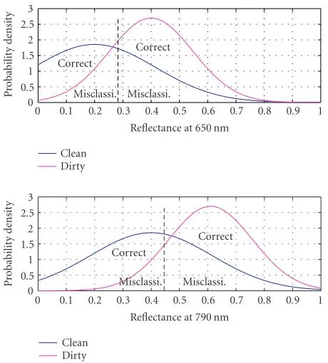
With two such distributions for the clean and unclean cases, respectively, the problem is to determine, from one or more measurements of reflectance, whether a given mea-surement represents a clean or an unclean area. This is il-lustrated inFigure 4where a measurement would be charac-terised as representing a clean area when reflectance is below the borderline between the two distributions. The figure also shows the probability for misclassification. In signal process-ing, measurement noise is often the prime source of misclas-sification and repeated measurements would be used to in-crease the likelihood that the right decision is made.

When noise is the prime nuisance, optimisation based on the Kullbak divergence is often used, for example, in a sym-metric version of the divergence [3]:

Di j=E

ln fi(r) fj(r)|θi

+E

ln fj(r)

fi(r)|θj

400 500 600 700 800 900 1000 Wavelength/nm

0 0.02 0.04 0.06 0.08 0.1 0.12 0.14 0.16 0.18 0.2

Re

fl

ec

ti

o

n

(a)

400 500 600 700 800 900 1000

Wavelength/nm 0

0.02 0.04 0.06 0.08 0.1 0.12 0.14 0.16 0.18 0.2

Re

fl

ec

ti

o

n

(b)

400 500 600 700 800 900 1000

Wavelength/nm 0

0.02 0.04 0.06 0.08 0.1 0.12 0.14 0.16 0.18 0.2

Re

fl

ec

ti

o

n

(c)

400 500 600 700 800 900 1000

Wavelength/nm 0

0.02 0.04 0.06 0.08 0.1 0.12 0.14 0.16 0.18 0.2

Re

fl

ec

ti

o

n

(d)

Figure3: Spectral data histograms for four selected materials: (a) concrete slab, (b) steel slab, (c) brown wood plate, (d) green plastic plate. Blue points indicate readings from clean surfaces, yellow/red points indicate readings from dirty surfaces. Darker colours correspond to a higher density of measurement data.

The problem at hand is peculiar, however, as the reason for uncertainty in data is not the measurement noise. As seen from the data plotted in Figures3ato3b, considerable vari-ance is caused by inhomogeneities in reflection from the in-dividual area segments of the clean surface. Simultaneously, there is even larger variation in the reflection caused by inho-mogeneous composition of the remains of dirt. One area may comprise specks with tiny remains of straw and solid parti-cles, others are covered by a thin layer of uniform contam-ination. Taking a number of identical pictures of each area element does not enhance information about the area and does not reduce the likelihood of misclassification.

For this reason, it would be advantageous to find a tech-nique of analysis by which the probability of misclassifica-tion Pe is minimised for each single area segment treated individually. As apparent from Figures3ato3d, the method

should cope with unequal dispersion matrices of distribu-tions for the clean and dirty cases.

The classical Mahalanobis measure [4] is a distance mea-sure between normal multidimensional distributions with equal dispersion. The Jeffreys-Matusita distance (JM dis-tance) [5] is a generalisation that applies to distributions with nonidentical dispersion and it does not require distributions to be normal. Further, it is possible to derive lower and up-per bounds for misclassification. Distance measures are dis-cussed in [3,6,7].

The Jeffreys-Matusita distance between distributions fi and fjis

Ji j=

Ω

fi(r)−fj(r) 2

dr 1/2

Misclassi. Misclassi. Correct Correct

0 0.1 0.2 0.3 0.4 0.5 0.6 0.7 0.8 0.9 1 Reflectance at 650 nm

0 0.5 1 1.5 2 2.5 3

P

robabilit

y

d

ensit

y

Clean Dirty

Misclassi. Misclassi. Correct Correct

0 0.1 0.2 0.3 0.4 0.5 0.6 0.7 0.8 0.9 1 Reflectance at 790 nm

0 0.5 1 1.5 2 2.5 3

P

robabilit

y

d

ensit

y

Clean Dirty

Figure 4: Distributions obtained at two distinct wavelengths for clean and dirty cases.

The JM distance measure has been found to be useful in a range of fields, from mineral classification [8] to identifica-tion of fungal colonies [9].

The JM distance isJi j = 0 when the distributions fi(r) and fj(r) are equal. The JM distance takes the value Ji j = √

2 when the two distributions are totally separated. Bhat-tachatyya introduced the coefficient

ρi j=

Ω

fi(r)fj(r)dr (7)

and used the negative logarithm,αi j, of this quantity:

αi j= −lnρi j. (8)

These have the obvious relation to the JM distance

J2 i j=2

1−ρi j=21−e−αi j ₍₉₎

Kailath [3] showed that when the two distributions are nor-mal multivariate of degreen: fi(r)= N(µi,Σi) and fj(r)= N(µj,Σj), then

αi j=1 8

µi−µjTΣ−1 i j

µi−µj

+1 2ln

detΣi j

detΣidetΣj,

(10)

where

Σi j=1

2

Σi+Σj

; (11)

the probability of misclassificationPeis bounded by

1 8ρ

2

i j≤Pe≤ρi j (12)

which is equivalent to

1 8

1−1 2J

2 i j

2

≤Pe≤1−1 2J

2

i j. (13)

The lower bound ofPeis reached whenJi j=√2 [3,6]. Salient features for the present context are the applica-bility of the JM measure to arbitrary distributions and the bounds for misclassification, although the analytic result of (13) is only an approximation when the distributions are not normal.

5.1. Multispectral techniques to reduce probability of misclassification

The JM distance measure will express the quality of a chosen technique to distinguish between the clean and nonclean sur-face cases. The complete spectra presented inSection 4were obtained using a dedicated spectrometer. For commonplace computer-vision techniques to be applied, we need to limit the number of frequencies analysed.

Figure 4 illustrates the theoretic distribution of re-flectance for the clean and nonclean cases if monochromatic light is used. The result is two normal distributions with a large overlap. If the discrimination was based on a single wavelength, the area would correspond to misclassification given the surface was clean:

Peθd|πc= 1

rsep

pr|πcdr, (14)

wherersepis shown as the dashed line inFigure 4. Misclassi-fication that the dirty surface was declared clean is shown:

Peθc|πd= _rsep

0 p

r|πddr. (15)

Using monochromatic or narrowband light at a single wave-length was found to give a rather large overlap between dis-tributions and hence a large probability of misclassification for all wavelengths when the surface is made of concrete.

0 2 4 6 8 10 12 14 P robabilit y d ensit y 1 0.8

0.6 0.4

0.2 0 Reflectanc

e at₆₅₀

nm 1 0.8

0.6 0.4 0.2 0

Reflectanc e at790

nm

Figure5: The two-dimensional normal distributions of clean and dirty areas are quite well separated and a low probability of misclas-sification is achieved.

0 0.5 1 1.5 Je ff re ys-M atusita distanc e

1000 900 ₈₀₀

700 ₆₀₀ 500 ₄₀₀ Wavelength/nm 400 500 600 700 800 900 1000 Wa vele ngt h/n m 1.2 1 0.8 0.6 0.4 0.2 0

Figure6: Jeffreys-Matusita distance computed for a range of can-didate wavelength pairs.

With this approach being promising, the formal ap-proach to design a sensor system should start with choosing two wavelengths, or more, that together give a desired low level of misclassification. Second, a method is needed to find the discriminator function to be used.

5.2. Best choice based on pig pen data

Comprehensive measurement data were obtained from a pig pen where different materials had been in use. The pen had been in use for three months when emptied. Part of the floor was made of newly finished concrete, other parts were 15 years old. Samples of the different materials were collected for analysis. 400 500 600 700 800 900 1000 W av elength 2 (nm)

400 500 600 700 800 900 1000

Wavelength 1 (nm)

20 18 16 14 12 10 8 6 4 2 0

5 5 10 15 ₂₀

5

5

1015 20 15 20 10 10 10 ₅ 5 ₅ 5 5 5 5

5 _{5 5}

Figure7: Upper bound of classification error as a function of wave-length pairs. The case is a concrete floor after 3-month use of the pen. Measurements were taken in a dry condition.

400 500 600 700 800 900 1000 W av elength 2 (nm)

400 500 600 700 800 900 1000

Wavelength 1 (nm)

20 18 16 14 12 10 8 6 4 2 0

5 10 ₁₅

5 10 20 5 10 15 20 2 2 5 10 10 5 15 10 20 20 15 2010 5 10 15 20 15 10 15 5 5 5 5 ₂₀ 10 15 20 2 5 10 15 2 5 10 15 5 5 10 ₂₀ 15 20

Figure8: Upper bound of classification error. The case is a 15-year-old concrete floor after 3-month contamination in the pen. Mea-surements were taken in a dry condition.

400 500 600 700 800 900 1000

W

av

elength

2

(nm)

400 500 600 700 800 900 1000

Wavelength 1 (nm)

20 18 16 14 12 10 8 6 4 2 0 20

15 10 10

20

15 10 5

15 20 20

20 1515 20 5

10 15

20

5 10 20

15 20

15 10

5

5 10

20 15

10 ₁₅ 20 10 5

10 15

20

Figure9: Upper bound of classification error as a function of wave-length pairs. The case is a concrete floor after 3-month use of the pen. Measurements were taken in a wet condition.

will be wet, and it is thus essential that discrimination can also be achieved in a wet condition.Figure 9shows the up-per bound for misclassification for the new floor in wet con-dition. The available ranges for illumination wavelength have now narrowed but good classification is still possible.

The analysis of large sets of experimental pig pen data have thus enabled a selection of illumination parameters to make good classification possible using multispectral dis-crimination.

5.3. Possibilities for improvement

In order to reduce the misclassification likelihood even fur-ther, it may be necessary to consider additional features to aid discrimination. Textural features, for example, could def-initely add relevant information under highly controlled cir-cumstances. However, variability in the image acquisition geometry—scale and orientation—for a practical scenario will contribute a significant amount of noise in textural fea-tures. In addition to this, it has been seen that the texture itself shows a high variation, and that there is a combined effect of this variation and the abovementioned variation in image acquisition geometry. This could develop into a highly complex texture study, which could be interesting, but which will almost certainly end up with a system less robust and general than a purely spectral system. The aim of this paper has been to check the potential of such a purely spectral sys-tem.

6. SENSOR DESIGN

The sensor is pixel based: each pixel is classified either as “clean” or “dirty.” The classification procedure is the Bayesian discriminant analysis, which assigns pixel measurements to classes from which they are most likely to have been pro-duced. The method relies on adequate knowledge of the statistics of the possible classifications, in this work the

mea-surements presented inSection 4form the basis of the dis-criminator.

The spectrographic characteristics of pig house sur-faces provide much more data than is expected from the camera-based sensor. The camera sensor provides a small number of channels, each described by the pair of fil-ter/illumination characteristics for the respective channel. In the design presented here, each channel is restricted to a nar-rowband of frequencies, produced, for example, by a number of powerful light-emitting diodes. The sensor collects im-ages corresponding to each channel in turn, by sequencing through the light sources for each channel. By synchronising the light sources to the camera’s frame rate, a set of images corresponding to a single two-dimensional measurement can be acquired in a relatively short time.

6.1. Wavelength selection

From the spectra presented inSection 4, a number of wave-lengths must be selected such that classification into clean and dirty classes for pig house surface materials is possi-ble. While some materials may be amenable to classification based on a single light colour (consider, for example, the green plastic inFigure 3dat around 490 nm or 620 nm), con-crete, the most important material, is clearly not. However, as illustrated previously, multidimensional analysis can reveal structure that is sufficient to discriminate classes.

Selecting the wavelengths 800 nm and 650 nm, for exam-ple, the surface characteristics can be illustrated in the scatter plot shown inFigure 10a. Four populations are shown, cor-responding to wet concrete and steel, in both clean and dirty conditions. As can be seen, with these wavelengths, clean and dirty concrete are well separated, whereas clean and dirty steel share a significant overlap. Selecting 650 nm and 450 nm on the other hand, as shown in Figure 10b, separates clean from dirty steel, but fails for concrete. Using all three wave-lengths, a discriminator can be constructed to handle both material types.

6.2. Bayesian discrimination

From the training data and the choice of wavelengths de-termined as just described, a number of populationsπi are modelled as normally distributed, multidimensional random variables:

πi←→Nµi,Σi. (16)

Using the experimental data,xi j, for each classi, estimates of the mean vectors and variance-covariance matrices for each population can be derived:

µi=1

n

j xi j,

Σi= 1

n−1

j

xi j−µixi j−µi.

(17)

2 3 4 5 6 7 8 9 10 11 12 Reflection at 650 nm (%)

0 2 4 6 8 10 12 14 16

R

eflection

at

800

nm

(%)

Clean concrete Dirty concrete

Clean steel Dirty steel (a)

0 2 4 6 8 10 12 14

Reflection at 450 nm (%) 2

3 4 5 6 7 8 9 10 11 12

R

eflection

at

650

nm

(%)

Clean concrete Dirty concrete

Clean steel Dirty steel (b)

Figure10: Scatter plots showing characteristics of concrete and steel in both clean and dirty states. Each plot shows two selected wavelengths, with each point corresponding to a single spectral measurement. Ellipses show one and two standard deviations for each material state. (a) Possible discriminator for concrete but not for steel—800 versus 650 nm. (b) Possible discriminator for steel but not for concrete—650 versus 450 nm.

associated. Bayes’ rule states that the probability that a mea-surementxis associated with the classπiis given by

Pπi|x=P

πiPx|πi

P(x) . (18)

A Bayesian classifier assigns a measurement to the class for which the probability calculated in (18) is the greatest. The termP(x|πi) is simply the probability distribution function for classi, which can be written asfi(x), andP(πi) is the prior probability of classi, which can written aspi. The denomi-natorP(x) is independent of the class, and is therefore irrel-evant with respect to maximising (18) across classes. Thus, a Bayesian classifier chooses the class maximising

Si= fi(x)pi, (19)

whereSiis being referred to as adiscriminant valueorscore. The termpiis thea prioriprobability of a measurement cor-responding to the population πi, and reflects knowledge of the environment prior to the measurement being taken.

In the case of multidimensional normal classes, the prob-ability density is given by

fi(x)=√1 2πn

1

detΣi e

−(1/2)(x−µi)Σ−i1(x−µi)_{. (20)}

Substituting this into (19) gives the discriminant value for the normally distributed case. In practise, the same decision

rule is achieved by applying a monotonic transformation to (19), so that

Si(x)=log pi detΣi

−1 2

x−µiΣ−i1

x−µi (21)

is minimised instead. Since this function is quadratic inx, it is known as a quadratic discriminant function.

7. A PROTOTYPE SENSOR

In order to demonstrate the proposed vision-based classi-fication method, a prototype sensor has been constructed. First, a colour digital video camera was used with white light in a seminatural environment. Subsequently, a monochrome camera with controlled multispectral lighting was used in a real pig house setting.

7.1. Seminatural environment

A prototype vision-based classifier was constructed us-ing readily available components—a desktop computer and colour digital video camera. The prototype demonstrates multivariable statistical classification using two of the three colour channels available in a normal colour image.

White reference Pixel mask

Live video window

Classification window

Class boundary Live video pixel

scatter plot Class variance/

covariance ellipse Pixel statistics

window

Figure11: Screen shot of prototype classifier. Top left: original camera image. Right: colour map—each dot corresponds to a pixel in the original image, increasing red intensity to the right and increasing blue intensity down. Bottom left: result of classification—each image pixel is now coloured to show its classification. The red area shows what will be cleaned. Ellipses in the right-hand window show trained class definitions.

A continuous lighting calibration is carried out by ensur-ing that one corner of the image has a known colour. The im-portance of this calibration underlines the necessity of con-trolled lighting for the actual sensor.

Figure 11 shows a screen shot of the prototype in ac-tion. Live video from the camera is displayed in the top-left window, two-dimensional colour statistics are shown in the right-hand window, and final pixel classifications are shown in the bottom-left window. The display is updated in real time, with a frame rate of 5 Hz.

A pixel mask is displayed in the video window, indicated with a circular, dashed black line. The user is free to re-size and move the mask, in order to select regions of inter-est. The large square window displays two types of informa-tion: statistics about the selected live video pixels and def-initions of previously learnt object classes. Video pixels are displayed as a scatter plot of white pixels with mean and vari-ance drawn on top in black. The background shows the de-fined object classes as strongly coloured ellipses, lighter ver-sions of the same colours show the regions the Bayesian clas-sifier associates with each class. Finally, the classification win-dow shows, for each pixel in the original image, which class the pixel is assigned to by the Bayesian classifier. The same colours are used as in the statistics window.

7.2. Pig house environment

In order to test the sensor design under realistic condi-tions, images of concrete surfaces from a working pig house were collected using a monochrome camera with controlled, strobe lighting. Two wavelengths were selected, one in the visible range—590 nm and one from the infrared one— 850 nm. Two images of each of two materials, clean and dirty concrete, were obtained. Each individual image con-tains 400 by 400 pixels, providing 160 000 individual mea-surements.

In order to test the method, a classifier was trained us-ing the first clean/dirty image pair and tested usus-ing the sec-ond image pair. Subsequently the pairs were swapped and the process repeated—twofold cross-validation.Figure 12shows

0 10 20 30 40

0 0.2

0.4 0.6

0.8 1 Re_flectanc

e_at 590

nm

1 0.8

0.6 0.4

0.2 0

Reflectance at 850 nm

Figure12: Histogram of clean and dirty pixel measurements from two concrete samples: the red surface shows the distribution of dirty pixel measurements, while the blue surface shows the distribution of clean pixel measurements.

the distributions obtained from the first image pair, which can be compared with the theoretical case presented earlier and illustrated inFigure 5.

The images obtained and the resulting classifications are shown inFigure 13. A simple median filter has also been ap-plied to the final classification to remove some of the classi-fication “noise,” particularly in the clean case. Misclassifica-tion in the clean case is expensive in the applicaMisclassifica-tion, since it results in wasted cleaning effort. Classification accuracy, both with and without the filter, is presented inTable 1. The error rates are in good agreement with the earlier analyses.

Figure13: Results of image classifications for two clean and dirty concrete samples. The first two columns show the raw images captured with light with wavelengths 590 nm and 850 nm, respectively. The third column shows the pixel-by-pixel classification, where blue pixels have been classified as clean and red as dirty. The fourth column shows the result of applying a five-by-five median filter to the classified image. The first two rows correspond to clean 1 and clean 2, respectively, whereas the third and fourth rows correspond to dirty 1 and dirty 2, respectively.

7.3. Algorithm

The program operation can be summarised more formally as follows.

Given

(1) A circular image mask with centre (mx,my) and radius mr.

(2) A list of classes,ck = (µk,Σk,pk,γk), with mean vec-tors, variance-covariance matrices, prior probabilities and display colours, respectively.

Initialisation

(1) Draw the scatter plot background showing class dis-crimination boundaries—calculate for each combina-tion of classcq and possible pixel measurementx = (I1I2),

Sqx= pq detΣqe

−(1/2)(x−µq)Σq−1(x−µq)_{, (22)}

and choose colourγkfor (I1,I2) such that

Skx=max

q Sqx. (23)

(2) Draw the class ellipses defined by µk and Σk using colourγk.

Repeat

(1) Read new image from camera:

X=

   

x11 . ..

xhw   

. (24)

(2) Update live image display withX.

(3) Compute meanµmand variance-covarianceΣmof the set of mask pixels given by

xm=xi j|i−my2+j−mx2≤m2 r

. (25)

(4) Update mask statistics in scatter display by drawing the ellipse defined byµmandΣm.

(5) Update scatter plot. Compute

sαβ=xi j=I1I2 _|

I1=α∧I2=β. (26)

sαβis the number of pixels measuring (αβ). Forsαβ > 0, plot a scatter plot pixel (α,β) with intensity increas-ing withs.

(6) Calculate, for each pixelxi jand classcq,

Sqx= pq detΣqe

Table1: Classification results for test images, with and without a median filter.

Sample Classification With filter

Clean Dirty Clean Dirty

Clean 0.996 0.004 0.999 0.001

Dirty 0.044 0.956 0.025 0.975

Update class display with

Y =

   

y11 . ..

yhw   

, (28)

choosingyi j=γksuch that

Skx=max

q Sqx. (29)

The computational requirements of the algorithm are modest, and the scenario envisioned for the cleaning robot does not require real-time performance. The prototype de-scribed here can process multiple frames per second with un-optimised desktop computer hardware, which is far beyond that which is actually required for a cleaning robot.

A partially offline procedure would also be acceptable, since it is expected that the cleaning and inspection phases will be staggered. The practical problems associated with protecting the sensor during cleaning, and capturing a suit-able image immediately after cleaning, mean that some time will elapse between a picture being taken and cleaning re-suming.

8. CONCLUSIONS

Based on strong incentives to replace manual labour in the cleaning of pig houses by a fully autonomous robot system, this paper analysed the key factors in the design of a vision-based sensor system to classify surfaces as clean or dirty. Spectral properties of floor and walls in pig houses were char-acterised using spectrometer measurements on clean and dirty surfaces. The raw spectral data showed a fairly high variation in reflection from dirty surfaces and direct dis-crimination was found to be impossible for surfaces made of concrete using any single wavelength in the visible or near-infrared ranges, 400–1100 nm, which were covered by the ex-perimental study. The key problem was shown to be varia-tion in reflecvaria-tion caused by the differences in surface mate-rial, and contamination, as a function of position, whereas fluctuation over time caused by measurement noise was mi-nor. Obtaining a low probability of misclassification for an observation of an element of the surface was therefore es-sential for the success of the concept. The paper employed the Jeffreys-Matusita distance measure and bounds on the misclassification probability to assess different scenarios for sensor design. An optimal choice of wavelengths for the il-lumination was calculated using actual field data and it was demonstrated that a probability below 2% was obtainable with just two different illumination wavelengths.

Design of a prototype algorithm to discriminate clean from dirty areas of a surface based on a Bayesian design of the multivariate classifier was demonstrated using a low-cost camera and standard computer interface. The results demon-strate the potential for designing a reliable and inexpensive vision system for autonomous pig house cleaning.

ACKNOWLEDGMENTS

The support of this research from the Sustainable Technol-ogy in Agriculture programme is gratefully acknowledged. The programme is funded jointly by the Danish Ministry of Science, Technology and Innovation and the Ministry of Food Agriculture and Fisheries under Grant number 2053-01-0021.

REFERENCES

[1] J. S. Strøm, G.-Q. Zhang, P. Kai, M. Lyngbye, I. Braithwaite, and S. Arrøe, “Intelligent sensor for autonomous cleaning of pig houses—system in context,” DJF Internal Rep. 182, Danish Institute of Agricultural Sciences, Tjele, Denmark, 2003. [2] H. B. Møller, S. G. Sommer, and B. K. Ahring, “Methane

pro-ductivity of manure, straw and solid fractions of manure,”

Biomass and Bioenergy, vol. 26, no. 5, pp. 485–495, 2004. [3] T. Kailath, “The divergence and Bhattacharyya distance

mea-sures in signal selection,”IEEE Transaction on Communication Technology, vol. 15, no. 1, pp. 52–60, 1967.

[4] B. K. Ersbøll and K. Conradsen, An Introduction to

Statis-tics, vol. 2, Informatics and Mathematical Modelling, Technical University of Denmark, Kongens Lyngby, Denmark, 2003. [5] K. Matusita, “A distance and related statistics in multivariate

analysis,” inMultivariate Analysis, P. R. Krishnaiah, Ed., pp. 187–200, Academic Press, New York, NY, USA, 1966.

[6] B. K. Nielsen, Transformations and classifications of remotely sensed data, Ph.D. thesis, Informatics and Mathematical Mod-elling (IMM), Technical University of Denmark, Kongens Lyn-gby, Denmark, 1989.

[7] J. Lin, “Divergence measures based on the Shannon entropy,”

IEEE Trans. Inform. Theory, vol. 37, no. 1, pp. 145–151, 1991. [8] H. Flesche, A. A. Nielsen, and R. Larsen, “Supervised mineral

classification with semiautomatic training and validation set generation in scanning electron microscope energy dispersive

spectroscopy image of thin sections,”Mathematical Geology,

vol. 32, no. 3, pp. 337–366, 2000.

[9] M. E. Hansen and J. M. Carstensen, “Density based retrieval

from high-similarity image databases,” Pattern Recognition,

vol. 37, no. 11, pp. 2155–2164, 2004.

Ian Braithwaitewas born in London,

Eng-land, in 1965. He received his B.A. (hon-ors) degree in control engineering from the University of Cambridge in 1988 and, af-ter moving to Denmark in 1993, received an M.S. degree from the Technical Univer-sity of Denmark in 1999. Mr. Braithwaite is currently employed as a Research Assis-tant at the Technical University of Den-mark, within the research project

Mogens Blankeis a Professor of automation at the Technical University of Denmark. He graduated from the Technical University of Denmark (DTU) in 1974, was with DTU in 1974–1975, at the European Space Agency in The Netherlands in 1975–1976, and again with DTU from 1976 till 1985. He received the Ph.D. degree from DTU in 1982. He was in the marine automation industry from 1985 to 1990 when he obtained the chair

as a Professor in control engineering at Aalborg University, Den-mark. He started his present position at DTU in 2000. His primary fields of interest are fault-tolerant control and diagnosis, modeling, and system identification. Application areas include autonomous robots, spacecraft, and surface ships. He has applied his research re-sults for autonomous attitude control for the Danish Ørsted satel-lite, for autopilot, platform, and maneuvering control, for mer-chant and naval vessels, and for adaptive diesel engine control. He has published results in about 150 articles and conference papers and in a recent textbook. He is an active member of IFAC, the In-ternational Federation of Automatic Control, where he served as a Technical Committee Chair for several years, and was a coordi-nating Chair and Member of the IFAC Council. He is also a Senior Member of the IEEE.

Guo-Qiang Zhangreceived the B.S. degree

in mechanical engineering from Jilin Uni-versity of Technology, Changchun, China, in 1982, and the Ph.D. degree in agricultural engineering from the Royal Veterinary and Agricultural University, Copenhagen, Den-mark, in 1989. He is currently a Senior Sci-entist at the Danish Institute of Agricultural Sciences and an Adjunct Professor in China Agricultural University. His research

inter-ests include indoor environmental and climatic control for live-stock buildings, process modeling, and experimental fluid dynam-ics. Dr. Zhang has over 70 international publications in the areas of agricultural and biosystems engineering. In his research career, he also evolved in many research activities on automation, remote sensing, and information technology in agricultural and biosys-tems process. He is a Member of the Danish Society of Engineers, Danish Society of Agricultural Engineering, and European Agricul-tural Engineering.

Jens Michael Carstensenreceived the M.S.

degree in engineering from the Technical University of Denmark, Lyngby, in 1988, and the Ph.D. degree in statistical image analysis from the Technical University of Denmark in 1992. He joined the Technical University of Denmark faculty in 1992 as an Assistant Research Professor and is cur-rently an Associate Professor. Since 1999, he has been the Chief Technical Officer and