R E S E A R C H
Open Access
Widely linear Markov signals
Juan A Espinosa-Pulido, Jes ´us Navarro-Moreno, Rosa M Fern´andez-Alcal´a
*and Juan C Ruiz-Molina
Abstract
The insufficiency to guarantee the existence of a state-space representation of the classical wide-sense Markov condition for improper complex-valued signals is shown and a generalization is suggested. New characterizations for wide-sense Markov signals which are based either on second-order properties or on state-space representations are studied in a widely linear setting. Moreover, the correlation structure of such signals is revealed and interesting results on modeling in both the forwards and backwards time directions are proved. As an application we give some
recursive estimation algorithms obtained from the Kalman filter. The performance of the proposed results is illustrated in a numerical example in the areas of estimation and simulation.
Keywords: Modeling, Wide-sense Markov signals, Widely linear processing
1 Introduction
Markov signals are characterized by the condition that future development of these signals depends only on cur-rent states and not their history up to that time. In general, Markov processes are easier to model and analyze, and they do include interesting applications. Among others, estimation and detection are areas of signal processing where this kind of process has provided efficient solu-tions (see, e.g., [1,2]). Non-Markov processes in which the future state of a process depends on its whole his-tory are generally harder to analyze mathematically [3]. In linear minimum-mean square error (MMSE) estima-tion theory, when the processes under consideraestima-tion are not Gaussian, the classes of stochastic processes which are of practical importance are wide-sense Markov (WSM) processes. The concept of WSM signal is easier to check than the condition of (strictly) Markov since it involves only second-order characteristics [4]. In general, WSM processes (with the exception of Gaussian processes) are not Markov in the strict sense. The equivalence between the WSM condition and the state-space representation for the signal is really what makes WSM signals especially attractive in signal processing [1].
Widely linear (WL) processing is an emerging research area in the complex-valued signal analysis which gives significant performance gains with respect to strictly linear (SL) processing (excellent account of the topic
*Correspondence: [email protected]
Department of Statistics and Operations Research, University of Ja´en, Campus Las Lagunillas, 23071 Ja´en, Spain
and the literature can be found in [5,6]). It has proved to be a more useful approach than SL processing since complex-valued random signals are in general improper (i.e., they are correlated with their complex conjugates). Thus, the improper nature of most signals forces us to consider the so-called augmented statistics to entirely describe their second-order properties. Using augmented statistics means incorporating in the analysis the informa-tion supplied by the complex conjugate of the signal and examining properties of both the correlation and com-plementary correlation functions. SL processing operates ignoring this last function. Some areas of signal process-ing in which the treatment of improper signals by usprocess-ing a WL processing has proved to be beneficial are estimation [5-11], detection [12], modeling [8], and simulation [13].
A general characteristic of the articles devoted to study-ing WSM complex-valued signals is that they use a SL processing approach (see e.g., [1,14-16]). We will show by means of simple examples that the classical definition and the associated characterizations of WSM signals are incorrect for improper signals. The examples then moti-vate the extension of the concept of WSM signal to a WL setting and the study of new characterizations. Specifi-cally, we introduce the concept of widely linear Markov (WLM) signals and we give different characterizations based either on second-order properties or on state-space representations from a WL processing point of view. The analysis is performed in both the forwards and back-wards directions of time. We also provide a way to check
the WLM condition, similar to the well-known triangu-lar property, based on augmented statistics and determine the correlation structure of WLM signals. The modeling part is the focus of this article. In this sense, WL forwards and backwards Markovian representations are suggested, the interrelation between them is studied and the connec-tion with the WL autoregressive representaconnec-tions defined in [8] is established. These Markovian representations also become a starting point for the application of different recursive estimation algorithms. Thus, the application of the Kalman filter on the forwards and backwards rep-resentations yields different WL prediction, filtering and smoothing algorithms. The point, which is illustrated in an example, is that besides the well-known performance gain of the WL approach we also get more realistic results in simulation and modeling.
The article is organized as follows. In Section 2, we present some background material on complex-valued Markov signals, illustrate the incapacity of the usual WSM condition in order to characterize the state-space repre-sentation for improper signals and suggest the concept of WLM signal. Some preliminary characterizations are also given. Section 3 studies the correlation structure of WLM signals. In Section 4, we discuss the modeling prob-lem for WLM signals and analyze the stationary case. The estimation problem is treated in Section 5. We apply our results in the fields of signal simulation and estima-tion by considering a numerical example in Secestima-tion 6. A Section of conclusions ends the article. To preserve con-tinuity in our presentation, all proofs are deferred to an Appendix 1.
2 Preliminaries
In this section, we give the main definitions, notation and auxiliary results. We also present two examples which motivate the necessity of the new concept introduced.
Bold capital letters will be used to refer to matrices and bold lower-case letters will be used to refer to vectors. The rowjof any matrixA(·)will be denoted byA[j](·), then
-vector of zeros by 0n and then×m-matrix of zeros by
0n×m. Furthermore, the superscripts∗,T, andHrepresent
the complex conjugate, transpose, and complex transpose, respectively.
Let{xt,t ∈ Z}be a zero-mean complex random signal
with correlation functionr(t,s) = E[xtx∗s] and
comple-mentary correlation functionc(t,s) = E[xtxs]. Most of
the results in this article are valid for nonstationary sig-nals. However, for some of them the stationary condition is necessary. The signal xt is said to be of second-order
wide-sense stationary (SOS) if the functions r(t,s) and c(t,s)depend ont−s. A zero-mean stochastic processwt
is called a doubly white noise ifE[wtw∗s]=e1δ(t−s)and
E[wtws]=e2δ(t−s)with|e2| ≤e1(see [8] for a complete
study of their characteristics). The linear MMSE estimator
ofxtbased on the set of observations{xt1,xt2,. . .,xtm}will be denoted byxˆ(t|t1,t2,. . .,tm)and we will refer to it as
the SL estimator.
The Markov condition on a signal{xt,t∈Z}establishes
the following identity for the conditional probability:
P(xt≤x|xt1,xt2,. . .,xtm)=P(xt≤x|xt1)
for all xandt > t1 > · · · > tm. Doob [4] introduced
a weaker concept based on the SL estimator which has received great attention in the literature (e.g., [1,14-16]). A signal xt is called WSM if xˆ(t|τ ≤ s) = ˆx(t|s) for
any s < t. Such signals have remarkable properties. For example, Beutler [14] showed that a signalxt is WSM if,
and only if, the functionk¯(t,s) = r(t,s)r−1(s,s) has the triangular property, i.e.,
¯
k(t,s)= ¯k(t,τ )k¯(τ,s), t≥τ ≥s (1)
Another characterization in terms of so-called Marko-vian state-space models can be found in [1]. They showed that a signal{xt,t ≥ 0} is WSM if, and only if, it has a
state-space model of the form
xt+1= ¯k(t+1,t)xt+ut (2)
where ut is a white noise uncorrelated with x0. Doob’s
definition was later generalized in [16] in the following sense:xtis a WSM signal of ordern ≥1 ifxˆ(t|τ ≤ s) =
ˆ
x(t|s,s−1,. . .,s−n+1)for anys <t. The authors also studied the second-order properties of such signals.
All these studies have a common characteristic: the information supplied by the complementary correlation function is ignored, i.e., the results are derived assuming implicitly that the signal is proper (c(t,s) = 0). As noted above, nowadays, the research activity in the field of the complex-valued signal is more and more focused on the better performing and less familiar WL processing. In this setting the SL MMSE estimator is replaced by the WL MMSE estimator, denoted byxˆWL(t|t1,t2,. . .,tm), which
uses the information of the augmented vector of observa-tions [xt1,x∗t1,xt2,x∗t2,. . .,xtm,x∗tm]
T. The immediate
ques-tion that arises is whether the classical concept of WSM signals remains valid in the WL processing approach. The following two examples give us the answer.
Example 1.Consider a signal {xt,t ≥ 0} with
corre-lation function r(t,s) = 12(e3|t−s| +e|t−s|) and
comple-mentary correlation function c(t,s) = 12(e3|t−s| −e|t−s|).
Example 2.Assume that{xt, 1 ≤ t ≤ 100}is a signal
with correlation and complementary correlation functions given by r(t,s) = (t/100+ 1)1/6(s/100)4 and c(t,s) = j(s/100)4, for s ≤ t, respectively, with j = √−1. Here, the triangular property (1) holds and then xt has the
representation
xt+1=
t+101 t+100
1/6
xt+ut (3)
with xtuncorrelated with ut. However, this model presents
two important shortcomings in the WL processing frame-work: the noise utis correlated with x∗tand the information
supplied by c(t,s)is ignored. Both problems can be avoided by considering a more competitive model for xt obtained
with the additional information of x∗t. In fact, we can write an alternative state-space representation for xt given by
(27). An exhaustive study about the superiority of (27) against (3) is presented in Section 6.
From these two simple examples we extract the fol-lowing consequences: the classical definition of a WSM signal must be extended to deal with improper signals, this new concept must be characterized adequately to avoid the drawback shown in Example 1 and new results about modeling are necessary to exploit the information avail-able in bothxtandx∗t thus attaining better models for the
signal as illustrated in Example 2. Next, we introduce such a definition in a WL processing setting.
Definition 1.A complex-valued signal{xt,t∈Z}is said
to be WLM of order n≥1, briefly a WLM(n) signal, if the following condition holds
ˆ
xWL(t|τ ≤s)= ˆxWL(t|s,s−1,. . .,s−n+1)
for any s<t.
Notice that this concept extends both the classical notion of WSM introduced by Doob in [4] and the later generalization given in [16].
In the rest of the section, we provide different charac-terizations of WLM(n) signals. For that, we need to intro-duce some additional notation. Denote the augmented forwards vector of ordern≥1 ofxtas the 2n-vector
xt=[xt,x∗t,xt−1,x∗t−1,. . .,xt−n+1,x∗t−n+1]T
and its correlation function byR(t,s) = E[xtxHs ]. From
now on, we assume that det{Rt} = 0 withRt := R(t,t).
Moreover, we define the normalized correlation function as
K(t,s)=R(t,s)R−s1 (4)
Similarly, we define the augmented backwards vector of ordern≥1 ofxtas the 2n-vector
xbt =[xt+n−1,x∗t+n−1,xt+n−2,x∗t+n−2,. . .,xt,x∗t]T
The following results establish the relation between the signalsxt and their augmented forwards and backwards
versions. We start first with the augmented forwards vec-tor and we give a test similar to (1) for a signal being WLM(n).
Theorem 1.The following statements are equivalent:
1. {xt,t∈Z}is a WLM(n) signal.
2. Fors<t, the WL MMSE estimator ofxton the basis
of the set{xτ,x∗τ,τ ≤s}is of the form
ˆ
xWL(t|τ ≤s)=K(t,s)xs (5)
3. Fort≥τ ≥s,
K(t,s)=K(t,τ )K(τ,s) (6)
Now, we suggest a characterization based on the aug-mented backwards vector. This result also shows the independence from the time direction of the Markov condition.
Theorem 2.The following statements are equivalent:
1. {xt,t∈Z}is a WLM(n) signal.
2. xˆWL(t|τ ≥s)= ˆxWL(t|s,s+1,. . .,s+n−1)for any
s>t.
3. Fors>t, the WL MMSE estimator ofxbt on the basis of the set{xbτ,xbτ∗,τ ≥s}is of the form
ˆ
xbWL(t|τ ≥s)=K(t+n−1,s+n−1)xbs (7)
3 Correlation structure of WLM(n) signals
In this section, the second-order properties of a WLM(n) signal{xt,t ∈ Z} are analyzed. Specifically, we study the
structure of the matrices R(t,s), K(t,s), Rt, and Kt :=
K(t+1,t).
Proposition 1. 1. The following relations hold:
K[2(j+i)−1](t+j,t)=
⎡ ⎢ ⎣0, . . ., 0
2i−2
, 1, 0, . . ., 0
2(n−i)+1
⎤ ⎥ ⎦,
j<n, i=1,. . .,n−j (8)
K[2(j+i)](t+j,t)=
⎡ ⎢ ⎣0, . . ., 0
2i−1
, 1, 0, . . ., 0
2(n−i)
⎤ ⎥ ⎦,
j<n, i=1,. . .,n−j (9)
K[2+i](t+j+1,t)=K[i](t+j,t),
K[1](t+j+1,t)=K[1](t+j+1,t+j)K(t+j,t),
j≥0 (11)
K[2](t+j+1,t)=K[2](t+j+1,t+j)K(t+j,t),
j≥0 (12)
2. The matrixKtis of the form
Kt= ⎡ ⎢ ⎢ ⎢ ⎢ ⎢ ⎢ ⎢ ⎢ ⎢ ⎢ ⎢ ⎢ ⎢ ⎣
k1,t k2,t k3,t k4,t · · · k2n−3,t k2n−2,t k2n−1,t k2n,t k∗2,t k1,t∗ k∗4,t k∗3,t · · · k2n∗−2,t k∗2n−3,t k∗2n,t k2n∗−1,t
1 0 0 0 · · · 0 0 0 0
0 1 0 0 · · · 0 0 0 0
. . . . . . . . . . . . . . . . . . . . . . . . . . .
0 0 0 0 · · · 1 0 0 0
0 0 0 0 · · · 0 1 0 0
⎤ ⎥ ⎥ ⎥ ⎥ ⎥ ⎥ ⎥ ⎥ ⎥ ⎥ ⎥ ⎥ ⎥ ⎦ (13)
whereki,t=ki(t+1,t)fori=1,. . ., 2nand
ki(t+1,t)is defined in (28).
3. The matricesR(t,s)andKtsatisfy the recursive
equation
R(t+1,s)=KtR(t,s), s≤t (14)
which has the solution
R(t,s)=Kt−1· · ·KsRs, s<t (15)
Moreover,
Rt+1=KtRtKHt +Qt
whereQtis a2n×2n-matrix of the form
Qt=
⎡ ⎢ ⎢ ⎣ At
02×2n−2
02n−2×2
02n−2×2n−2
⎤ ⎥ ⎥
⎦ (16)
with
At=
a1,t a2,t
a∗2,t a1,t
wherea1,tare real positive numbers andAtis
nonnegative definite.
4 Modeling of WLM(n) signals
We aim to provide different ways of modeling for WLM(n) signals. The connection between stationary WLM(n) sig-nals and the autoregressive representations defined in [8] is also established. First, we present a new characteriza-tion in which the equivalence between a WLM signal of ordernand their forwards and backwards representations is given. Such representations show that a WLM(n) signal depends only on thenpreceding or subsequent states and their conjugates.
Theorem 3.A signal{xt, 0 ≤ t ≤ m}is a WLM(n)if,
and only if, it has the forwards and backwards representa-tions
xt+1=kTtxt+wt, t≥n−1 (17)
xt=kbTt+1xbt+1+wbt+1, t≤m−n+1 (18)
wherekt, kbt are2n-vectors, and wt, wbt are doubly white
noises such that
E[wtxn−1]=02n, t≥n−1 (19)
E[wbtxbm−n+1]=02n, t≤m−n+1
Now we state a parallel result to the classical one estab-lished for stationary WSM processes and autoregressive representations [16].
Corollary 1. If{xt, 0≤t≤m}is a SOS WLM(n) signal,
then xtis the solution of the WL system defined in [8]
xt+1= n−1
i=0
g1,ixt−i+ n−1
i=0
g2,ix∗t−i+wt (20)
where g1,i,g2,i ∈ C, i = 1,. . .,n−1, and wt is a doubly
white noise such that E[wtw∗t]=a1and E[wtwt]=a2.
We summarize the previous results in the following steps which provides forwards and backwards models for a WLM(n) signal:
Step 1:Define the2n-vectorktsuch thatkTt
coincides with the first row of the matrix
Kt:=R(t+1,t)R−t1 (21)
Similarly, we define the2n-vectorkbt+1such that kbTt+1is equal to the2n−1row of the matrix
Kbt+1:=K(t+n−1,t+n)=R(t+n−1,t+n)R−t+1n (22)
Step 2:Consider the matrices
Qt=Rt+1−KtRtKHt (23)
Qbt+1=Rt+n−1−Kbt+1Rt+nKbHt+1 (24)
Step 3:The signalxtcan be represented by the
following forwards and backwards models:
xt+1=kTtxt+wt, t≥n−1
xt=kbTt+1xbt+1+wbt+1, t≤m−n+1
wherewtis a doubly white noise uncorrelated with
xn−1for allt≥n−1andwbt is a doubly white noise
uncorrelated withxm−n+1for allt≤m−n+1.
(1,1)-element and (1,2)-element of the matrixQt, respectively. Similarly,E[wbtwbt∗]andE[wbtwbt]are the(2n−1, 2n−1)-element and
(2n−1, 2n)-element of the matrixQbt, respectively.
In certain situations we have a forwards model of the form (17) for the signal xt. It would be interesting to
be able to obtain a backwards model directly from the forwards model. Next, we show a useful way to get our objective.
Proposition 2.Given a forwards model of the form
xt+1=kTtxt+wt, n−1≤t≤m (25)
with wta doubly white noise uncorrelated withxn−1, then
{xt, 0≤t≤m}has the backwards representation
xt=kbTt+1xbt+1+wbt+1, 0≤t≤m−n+1
where the2n-vectorkbt+1satisfies thatkbTt+1is equal to the 2n−1row of the matrixKbt+1=Rt+n−1KHt+n−1R−t+1nand
wbt is a doubly white noise with the properties given in Step 3 above.
Example 1(continued).It is not difficult to check that xtis a WLM(1) signal by using property (6). Hence,
apply-ing Steps 1–3 above, it has the state-space representation
xt+1=
1 2(e
3+e)x t+
1 2(e
3−e)x∗
t +wt (26)
with wta doubly white noise uncorrelated with x0and x∗0.
Moreover, as xtis also a SOS signal, this model is trivially
its WL autoregressive representation.
Example 2(continued).From Theorem 1 and Steps 1– 3, it follows that xtis a WLM(1) signal and has the
state-space representation
xt+1=
101/3(t+101)1/6(t+100)1/6−10 101/3(t+100)1/3−10 xt
+j10
2/3(−(t+101)1/6+(t+100)1/6)
101/3(t+100)1/3−10 x
∗
t+wt
(27)
with wta doubly white noise uncorrelated with x1and x∗1.
5 Estimation problem of WLM(n) signals
Once the modeling problem has been solved for WLM(n) signals, we address the MMSE estimation problem of such signals under a WL processing approach. The for-wards and backfor-wards representations given in Theorem 3 notably simplify the design of different recursive estima-tion algorithms. To this end, we use the Kalman recursions on the forwards representation to provide the solution for
the prediction and filtering problems and on the back-wards representation for the smoothing problem (see, e.g., [17,18]).
Suppose that we observe a WLM(n) signal{xt, 0≤t ≤
m}via the process
yt=htxt+vt, 0≤t≤m
withvta doubly white noise such thatE[vtv∗t]= n1,tand
E[vtvt]=n2,twithn1,t>|n2,t|. Moreover, we assume that
vtis uncorrelated withxsandx∗s for allt,s.
Consider the 2-vectoryt=[yt,y∗t]T, the 2×2nmatrix
Ht=
ht 0 0 · · · 0
0 h∗t 0 · · · 0
and the 2×2 matrix
Nt=
n1,t n2,t
n∗2,t n1,t
5.1 Prediction and filtering cases
Denote the WL filtered estimator of xt by xˆWLt and the
one-step-ahead predictor ofxt+1byxˆWLt+1|t, both obtained
on the basis of the information provided by the set {y0,y∗0,. . .,yt,y∗t}, and consider their associated errors
pt = E[|xt − ˆxWLt |2] and pt+1|t = E[|xt+1− ˆxWLt+1|t|2].
Also denote the estimate ofxn−1obtained from the
infor-mation provided by [yn−1,y∗n−1,. . .,y0,y∗0]T byxˆn−1and
its associated error byPn−1. By combining the forwards
representation (17) and the classical Kalman filter we present Algorithm 1 which provides these estimators in an efficient way.
Algorithm 1. WL filter and prediction
Require: yt,Ht,Nt,Kt,Qt,g =[ 1, 0,. . ., 0]T,xˆn−1, and
Pn−1
Ensure:xˆWLt+1|t,xˆWLt+1,pt+1|t, andpt+1
5.2 Smoothing case
Next, we compute two WL smoothing estimators of xt
and it will be denoted by xˆbtWL. The second one is derived from the information supplied by the set {yt+1,y∗t+1,. . .,ym,y∗m} and we will refer to it as xˆb
WL t|t+1.
The errors of both estimators arepbt = E[|xt− ˆxb WL t |2]
and pbt|t+1 = E[|xt − ˆxb WL
t|t+1|2], respectively. The
ini-tial conditionxˆbm−n+1is the estimate ofxbm−n+1obtained from the 2n+2-vector [ym−n+1,y∗m−n+1,. . .,ym,y∗m]Tand
Pbm−n+1is its associated error. By applying the backwards Kalman recursions on the backwards model (18) we get Algorithm 2.
Algorithm 2. WL smoothing
Require: yt, Ht, Nt, Kbt+1, Qbt+1, l =[ 0,. . ., 0, 1, 0]T,
ˆ
xbm−n+1, andPbm−n+1
Ensure:xˆbt|WLt+1,xˆtbWL,pbt|t+1, andpbt
6 Numerical example
This section is devoted to showing the advantages of rep-resentation (27) (model 2) in relation to (3) (model 1) in two fields of signal processing: simulation and estima-tion. Firstly, we use such models to simulate trajectories of xt defined in Example 2. Specifically, 50,000
trajecto-ries of both models have been generated via Montecarlo simulation. To assess the performance of the simulations we compare the true correlation and complementary cor-relation functions with the simulated ones. Figure 1a,b depicts the true correlation and complementary correla-tion funccorrela-tions ofxt, Figure 1c,d the simulated simulated
ones corresponding to model 1 and Figure 1e,f the sim-ulated ones for model 2. We can see that the simsim-ulated trajectories of model 1 pick up adequately the behavior of the correlation function. However, these trajectories are unable to show the basic characteristics of the comple-mentary correlation function. This shortcoming does not appear with model 2 whose simulated trajectories yield accurate representations of the second-order moments of xt. For more detail, the 2D sections of the true
comple-mentary function and the simulated ones with models 1
and 2 fort = 60 andt = 90, respectively, are shown in Figure 2a,b.
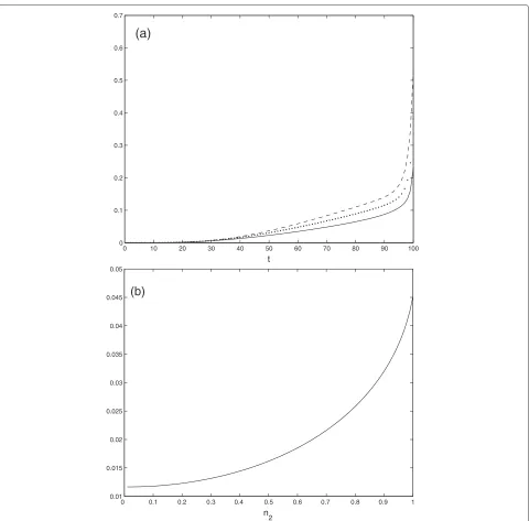
Finally, we compare the SL smoother obtained with model 1 and the WL smoother derived in Algorithm 2 for model 2. For the particular case in which ht = 1
andn1,t = 1, Figure 3a compares the errorpbt obtained
forn2,t = 0.25 (dotted line) and n2,t = 0.8 (solid line)
with the counterpart SL error (dashed line). On the other hand, considering n2t = n2 and denoting the errors of
the improper and proper smoothers for every value ofn2
bypbt(n2)andp¯bt(n2), respectively, Figure 3b displays the
mean of the difference between the SL and WL estimation errors, that is,DE(n2)= 1001 100t=1(p¯bt(n2)−pbt(n2))with
n2 varying within the interval [ 0, 1). As expected, both
figures show that WL estimation outperforms SL estima-tion, that is, they illustrate the better performance of the improper smoother in relation to the proper one. From Figure 3b, we also come to the conclusion that this gain in performance decreases asn2reduces.
7 Conclusions
The limited utility of the classical WSM definition to char-acterize the existence of a state-space representation for improper random signals has been revealed. By means of two simple examples, we have shown that in some cases the triangular condition fails to hold for signals with a state-space representation or that there exist signals with autocorrelations satisfying the triangular property for which the associated state-space representations present drawbacks in relation to their WL counterparts. Thus, the definition of a WSM signal has been extended to deal with improper signals providing new characterizations for WLM signals based either on second-order proper-ties or on state-space representations. Moreover, a way to check the WLM condition has been given and the corre-lation structure of WLM signals has been devised. Finally, WL forwards and backwards Markovian representations have been presented from which some applications are illustrated in the signal estimation and simulation fields.
Appendix 1
Proof of Theorem 1
To prove the implication 1) ⇒ 2) observe that ifxt is a
WLM(n) signal then for anys<t,
ˆ
xWL(t|τ ≤s)=k1(t,s)xs+k2(t,s)x∗s + · · ·
+k2n−1(t,s)xs−n+1+k2n(t,s)x∗s−n+1
(28)
10 20 30 40
50 60 70 80
90 100
20 40 60 80 100
0.2 0.4 0.6 0.8 1
s (a) True correlation function
t z
20 40
60 80
100
20 40 60 80 100
0.2 0.4 0.6 0.8 1
s (b) True complementary function
t z
20 40
60 80
100
20 40 60 80 1000 0.2 0.4 0.6 0.8 1
s
(c) Simulated correlation function for model 1
t z
20 40
60 80 100
20 40 60 80 100−7
−6 −5 −4 −3 −2 −1 0 1
x 10−3
s
(d) Simulated complementary function for model 1
t z
20 40
60 80
100
20 40 60 80 1000 0.2 0.4 0.6 0.8 1
s
(e) Simulated correlation function for model 2
t z
20 40
60 80
100
20 40 60 80 1000 0.2 0.4 0.6 0.8 1
s
(f) Simulated complementary function for model 2
t z
0 10 20 30 40 50 60 70 80 90 100 −0.02
0 0.02 0.04 0.06 0.08 0.1 0.12 0.14
s
True complementary function for t=60 Simulated complementary function for model 2 Simulated complementary function for model 1
0 10 20 30 40 50 60 70 80 90 100 −0.1
0 0.1 0.2 0.3 0.4 0.5 0.6 0.7
s True complementary function for t=90
Simulated complementary function for model 2 Simulated complementary function for model 1
Figure 2 (a)2D section of true and simulated complementary functions fort=60:(b)2D section of true and simulated complementary functions fort=90.
K[2i−1](t,s)=[k1(t−i+1,s),k2(t−i+1,s),. . .,k2n−1
×(t−i+1,s),k2n(t−i+1,s)]
K[2i](t,s)=
k2∗(t−i+1,s),k∗1(t−i+1,s),. . .,k2∗n
×(t−i+1,s),k2∗n−1(t−i+1,s) (29)
for i = 1,. . .,n. The inverse implication, 2) ⇒ 1), is checked similarly.
Finally, the proof of 2)⇔ 3)is similar to the one given in Theorem 1 of [16].
Proof of Theorem 2
The proof of 2) ⇔ 3)is similar to that of Theorem 1 by taking into account thatE[xbtxbsH]=R(t+n−1,s+n−1). Now, we prove 1) ⇔3). Following a similar reasoning to that used in the proof of Theorem 1 in [16], we have that
(7) is equivalent to the condition
K(t,s)=K(t,τ )K(τ,s), t≤τ ≤s
and thus,
KH(s,t)=KH(τ,t)KH(s,τ )=(K(s,τ )K(τ,t))H,
t≥τ ≥s
from which, applying Theorem 1, it follows that xt is a
WLM(n) signal. In a similar way the implication 1) ⇒3) is proven.
Proof of Proposition 1
Taking into account thatxˆWL(t+j−i|τ ≤t)=xt+j−ifor
0 10 20 30 40 50 60 70 80 90 100 0
0.1 0.2 0.3 0.4 0.5 0.6 0.7
(a)
t
0 0.1 0.2 0.3 0.4 0.5 0.6 0.7 0.8 0.9 1 0.01
0.015 0.02 0.025 0.03 0.035 0.04 0.045 0.05
(b)
n 2
Figure 3 (a)Smoothing errors: WL smoothing errorspbtforn2,t=0.25(dotted line) andn2,t=0.8(solid line), and the SL smoothing error (dashed line):(b)Performance of the smoother estimate.Mean of the difference between the SL and WL estimation errors DE(n2).
Now, from (6) we get
K(t+j+1,t)=K(t+j+1,t+j)K(t+j,t), j≥0
and together with (13) we demonstrate (10), (11), and (12). On the other hand, (14) and (15) can be proven follow-ing a similar reasonfollow-ing to that of Theorem 2 in [16].
Finally, by using the Hilbert projection theorem and (5) we have
xt+1=Ktxt+wt (30)
wherewt =[wt,w∗t, 0,. . ., 0]T is the innovations process
which, by construction, is uncorrelated withxsfort ≥s.
Thus,
Rt+1=E
xt+1xHt+1
=E(Ktxt+wt) (Ktxt+wt)H
=KtRtKHt +Qt
Proof of Theorem 3
Ifxtis a WLM(n) signal then, from (13) and (30), we have
xt+1=k1,txt+k2,tx∗t + · · · +k2n−1,txt−n+1
+k2n,tx∗t−n+1+wt
(31)
where wt is the first component ofwt. Hence, denoting
kt = KT[1](t+1,t) =[k1,t,. . .,k2n,t]T we obtain (17). On
the other hand, from the Hilbert projection theorem and (7) we get
xbt =K(t+n−1,t+n)xbt+1+wbt+1 (32)
wherewbt =[ 0,. . ., 0,wbt,wbt∗]T is the backwards innova-tions process which, from construction, is uncorrelated with xs fort ≤ s. Hence, xt = K[2n−1](t +n−1,t +
n)xbt+1+wbt+1withwbt+1the 2n−1 component ofwbt+1.
Thus, denotingkbTt+1= K[2n−1](t+n−1,t+n), (18) is
obtained.
Conversely, suppose thatxthas the representation (17).
DenoteHthe closed span generated by the set{xτ,x∗τ,τ ≤ t}. By using Proposition 2.3.2 of [19], to prove that ˆ
xWL(t|τ ≤s)= ˆxWL(t|s,s−1,. . .,s−n+1)for anys<tis
equivalent toxˆWL(t+1|τ ≤t)= ˆxWL(t+1|t,t−1,. . .,t−
n+1) for allt. Thus, projecting (17) ontoHand taking Proposition 2.3.2 of [19] into account we have
ˆ
xWL(t+1|τ ≤t)=kTtxt+ ˆwWL(t|τ ≤t)
wherewˆWL(t|τ ≤ t)is the projection ofw
tontoH. The
hypothesis (19) guarantees thatwtis uncorrelated withxs
andx∗s fort ≥ s. Hence,wˆWL(t|τ ≤ t) = 0 andxt is a
WLM(n) signal.
The proof for the backwards representation (18) is similar.
Proof of Corollary 1
Sincextis a SOS signal then the matricesR(t+h,t),h=
1, 2,. . ., are independent oft. Thus, from (4) we obtain ki,t=kifor alliandt. Finally, taking (31) into account we
have
xt+1= n−1
i=0
k2i+1xt−i+ n−1
i=0
k2i+2x∗t−i+wt
which gives (20) definingg1,i=k2i+1andg2,i=k2i+2.
Proof of Proposition 2
From (25) and Theorem 3 it follows that xbt has the representation (32). Then by using (22) we obtain
Kbt+1=K(t+n−1,t+n)=R(t+n−1,t+n)R−t+1n
=RH(t+n,t+n−1)R−t+1n=Rt+n−1KHt+n−1R−t+1n
and thus the result follows.
Abbreviations
MMSE, Minimum-mean square error; SL, Strictly linear; WL, Widely linear; WLM, Widely linear Markov; WSM, Wide-sense Markov.
Competing interests
The authors declare that they have no competing interests.
Received: 28 May 2012 Accepted: 29 October 2012 Published: 18 December 2012
References
1. T Kailath, AH Sayed, B Hassibi,Linear Estimation. (Prentince Hall, New Jersey, 2000)
2. HV Poor, Ch Chang, A reduced-complexity quadratic structure for the detection of stochastic signals. J. Acoust. Soc. Am.78(5), 1652–1657 (1985) 3. PW Jones, P Smith,Stochastic Processes. An Introduction. (Chapman &
Hall/CRC, Boca Raton, 2010)
4. JL Doob,Stochastic Processes. (John Willey, New York, 1953) 5. DP Mandic, VSL Goh,Complex Valued Nonlinear Adaptative Filters.
Noncircularity, Widely Linear and Neural Models. (John Willey, New York, 2009)
6. T Adali, S Haykin,Adaptive Signal Processing: Next Generation Solutions. (Wiley-IEEE Press, New York, 2010)
7. J Navarro-Moreno, MD Estudillo, RM Fern´andez-Alcal´a, JC Ruiz-Molina, Estimation of improper complex-valued random signals in colored noise by using the hilbert space theory. IEEE Trans. Inf. Theory.55(6), 2859–2867 (2009)
8. B Picinbono, P Bondon, Second-order statistics of complex signals. IEEE Trans. Signal Process.45(2), 411–420 (1997)
9. VSL Goh, DP Mandic, An augmented extended kalman filter algorithm for complex-valued recurrent neural networks. Neural Comput.19, 1039–1055 (2007)
10. J Navarro-Moreno, ARMA prediction of widely linear systems by using the innovations algorithm. IEEE Trans. Signal Process.56(7), 3061–3068 (2008) 11. C Cheong Took, DP Mandic, A quaternion widely linear adaptive filter.
IEEE Trans. Signal Process.58(8), 4427–4431 (2010)
12. S Buzzi, M Lops, S Sardellitti, Widely linear reception strategies for layered space-time wireless communications. IEEE Trans. Signal Process.54(6), 2252–2262 (2006)
13. P Rubin-Delanchy, AT Walden, Simulation of improper complex-valued sequences. IEEE Trans. Signal Process.55(11), 5517–5521 (2007) 14. F Beutler, Multivariate wide-sense Markov processes and prediction
theory. Ann. Math. Stat.34(2), 424–438 (1963)
15. V Mandrekar, On multivariate wide-sense Markov processes. Nagoya Math. J.3, 7–19 (1968)
16. A Kasprzyk, W Szczotka, Covariance structure of wide-sense Markov processes of orderk≥1. Appl. Math.33(2), 129–143 (2006)
17. DH Dini, DP Mandic, SJ Julier, A widely linear complex unscented Kalman filter. IEEE Signal Process. Lett.18(11), 623–626 (2011)
18. DH Dini, DP Mandic, Class of widely linear complex Kalman filters. IEEE Trans. Neural Netw. Learn. Syst.23(5), 775–786 (2012)
19. PJ Brockwell, RA Davis,Time Series: Theory and Methods, 2nd edn. (Springer-Verlag, New York, 1991)
doi:10.1186/1687-6180-2012-256
Cite this article as:Espinosa-Pulidoet al.:Widely linear Markov signals.